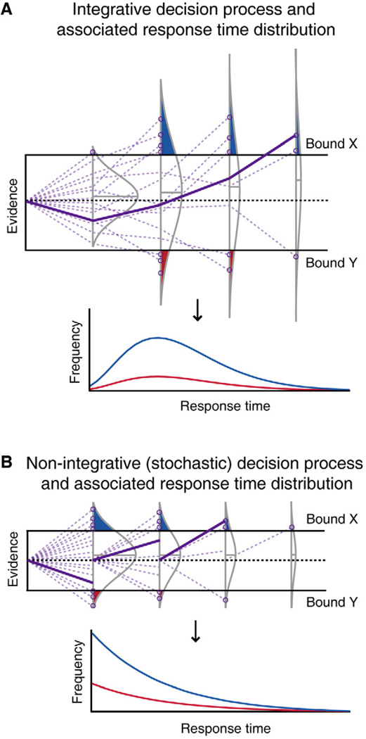
Figure 2. Integrative and non-integrative models of decision-making generate different predictions about RT probability distributions.

(A) In an integrative decision process, successive samples of information, or “evidence,” are accumulated over time, and a choice is made when that evidence crosses one of two decision bounds (X or Y, upper panel). This schematic shows integration of evidence (purple lines) for 16 example trials, each terminating in a choice of X or Y (purple circles). Normal curves (grey lines) represent the distribution of evidence levels after each of 4 samples (simulated across many trials), where the shaded areas of the curves represent relative numbers of choices made at each sampling point for either X (blue) or Y (red). This decision process can be transformed into RT distributions for choices X (blue line) and Y (red line), which conform to gamma-distributed probability density functions (lower panel). (B) In a non-integrative (stochastic) decision process, each sample of information is independent of the previous samples, and a choice is made when a single sample has sufficient evidence to cross a bound (upper panel). The schematic also depicts 16 example trials with 4 sampling points, but in this instance, if evidence does not surpass a threshold level, the decision process begins again at zero evidence for the next sample. The RT distributions arising from this non-integrative process (lower panel) conform to exponentially decaying probability density functions. Specific example trials (solid purple lines) in the upper panels of (A) and (B) depict differences in how evidence accrues over time in the two models.