An Atlas-Based Geometry Pipeline for Cardiac Hermite Model Construction and Diffusion Tensor Reorientation

Abstract

Here we present a novel atlas-based geometry pipeline for constructing three-dimensional cubic Hermite finite element meshes of the whole human heart from tomographic patient image data. To build the cardiac atlas, two superior atria, two inferior ventricles as well as the aorta and the pulmonary trunk are first segmented, and epicardial and endocardial boundary surfaces are extracted and smoothed. Critical points and skeletons (or central-line paths) are identified, following the cardiac topology. The surface model and the path tree are used to construct a hexahedral control mesh via a skeleton-based sweeping method. Derivative parameters are computed from the control mesh, defining cubic Hermite finite elements. The thickness of the atria and the ventricles is obtained using segmented epicardial boundaries or via offsetting from the endocardial surfaces in regions where the image resolution is insufficient. We also develop a robust optical flow approach to deform the constructed atlas and align it with the image from a second patient. This registration method is fully-automatic, and avoids manual operations required by segmentation and path extraction. Moreover, we demonstrate that this method can also be used to deformably map diffusion tensor MRI data with patient geometries to include fiber and sheet orientations in the finite element model.

1. Introduction

Many advances in computational modeling and biomechanics over the past two decades have taken advantage of smooth high-order cubic Hermite finite elements (Bradley et al., 1997; Legrice et al., 2001; Hunter et al., 2003; Kerckhoffs et al., 2006), which allow cardiac geometry to be discretized accurately with comparatively few degrees of freedom. Owing to advances in non-invasive imaging technology, it is now a feasible goal to create patient-specific models to provide insight into disease processes like ventricular arrhythmia, atrial fibrillation and congestive heart failure. Generating accurate geometries from medical images (Zhang and Bajaj, 2004; Zhang et al., 2005) is well-studied when the resultant geometry is composed of linear (especially tetrahedral) elements but is more challenging for high-order C¹-continuous finite elements.

Most work on generation of high-order cardiac geometries from image data have focused on relatively simple geometries such as the chest wall, lungs, and cardiac ventricles (Lamata et al., 2011), and relied on user-input parameter values that cannot always be anticipated a priori (Bradley et al., 1997). Cubic Hermite models were previously used to register DTI and strain data and solve the inverse cardiac mechanics problem (Wang et al., 2009). Additionally, though some cubic Hermite models of the heart have been constructed with more complicated topologies such as the valve annuli (Stevens and Hunter, 2003), construction of such meshes can be labor-intensive. The construction of an accurate four-chamber geometric model based on cubic Hermite splines would require a tremendous amount of user input to create the hexahedral mesh connectivity that represents the topology of four chambers and great vessels.

Here we describe a novel atlas-based geometry pipeline for constructing three-dimensional cubic Hermite finite element meshes of the human heart from non-invasive medical images, taking into account details of the whole heart structure, including four chambers and all major blood vessels. Note that valve annuli are not yet considered in the model. Our algorithm makes use of minimal user interaction to create the cardiac atlas based on the skeleton of a patient’s heart. Once this atlas is obtained, we can create cardiac meshes for different patients using deformable registration. The key contributions include: (1) a novel atlas-based geometry pipeline to construct cubic Hermite models for the whole heart; (2) a unique 1D center-line path tree to represent the complex cardiac topology and decompose the heart into simple components, which are meshed individually and connected to build the atlas; and (3) a robust and fully-automatic optical flow approach to deform the constructed atlas to match with new patients’ images, as well as register diffusion tensor MRI data to include fiber and sheet orientation into finite element models. The constructed Hermite meshes are suitable for cardiac mechanical and electrical function analysis, due to their convergence advantages over linear elements for nonlinear large deformation biomechanical simulation (Costa et al., 1996) and monodomain modeling of cardiac action potential propagation (Rogers et al., 1996).

2. Atlas-Based Geometry Pipeline

Three patients who gave informed contact underwent electrocardiogram-gated 64-slice CT with an iodine-based contrast agent as part of clinical evaluation for atrial fibrillation. Contiguous slices of 1.25mm were obtained along the axis of the scanner, with in-plane resolutions of 0.7mm by 0.7mm for Patient 1. For Patients 2 and 3, the resolutions are 0.48mm ×0.48mm ×0.65mm. As shown in Fig. 1, we used images from one patient (Patient 1) to construct the atlas. Four cardiac chambers and all major vessels were manually segmented using ITK-SNAP (www.itksnap.org) with intensity gradients as a guide (Yushkevich et al., 2006). From the segmented images, the luminal surface was extracted via isocontouring coupled with geometric flow smoothing (Zhang et al., 2009) for the two atria, the aorta and the pulmonary trunk. Due to the lack of resolution and contrast with current in-vivo imaging technology, it is often difficult to extract their thicknesses from clinical images. For the ventricles, the epicardial and endocardial boundary surfaces were extracted and smoothed. After the surface models were obtained, the skeleton (or center-line path) for each component was extracted with some user interaction, defining the cardiac topology. The hexahedral control mesh was constructed via a skeleton-based sweeping method (Zhang et al., 2007), and solid cubic Hermite finite element parameters were derived from the control mesh directly.

Figure 1.

A schematic diagram of the atlas-based geometry pipeline.

For images from the subsequent two patients, instead of repeating these steps, we made use of the atlas model from the first patient to generate new patient meshes automatically. For each new patient, a robust optical flow approach was developed to deform the hexahedral control mesh of the constructed atlas to match it with the new patient’s images. This avoids the manual operations required for segmentation and path extraction.

3. Atlas Construction via Sweeping

For the first patient, we obtain a surface model from the segmented images, see Fig. 2, and a cubic Hermite atlas is constructed via the following steps: path extraction, control mesh, and cubic Hermite construction.

Figure 2.

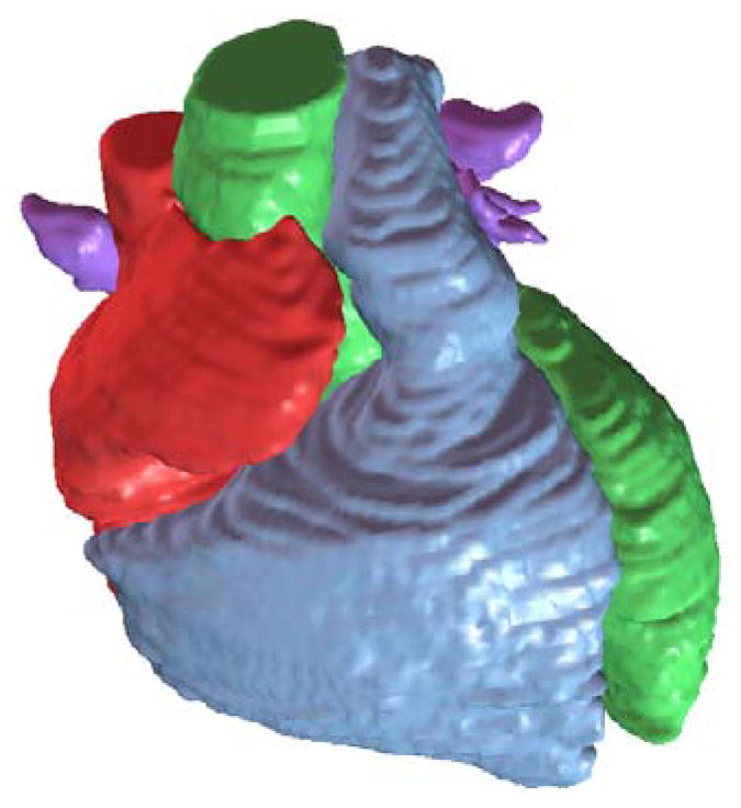
Segmented heart with four chambers, the aorta and the pulmonary trunk.

3.1. Path Extraction

Reeb-graphs (Reeb, 1946) have been used to analyze surface topologies and construct medial axes or skeletons (Lazarus and Verroust, 1999). As reviewed by Cornea et al. (2005a), there are a lot of techniques developed for skeleton extraction, including topological thinning (Borgefors et al., 1999), distance field based methods (Zhou and Toga, 1999), potential field based methods (Cornea et al., 2005b), thinning via medial geodesic function (Dey and Sun, 2006) and others (Verroust and Lazarus, 2000). Here we chose the critical point theory of the distance function (Zhang et al., 2007) to define a novel skeleton (or central path) tree for the whole cardiac model, following the blood flow path inside the heart and the cardiac anatomy structure. The primary principle we comply with is the “equidistant rule”, which means the skeleton point in a certain cross section should be the centroid of that cross section. Owing to the quasi-tubular anatomical structure of the four chambers, we can conveniently calculate the centroid at an arbitrary axial cross section perpendicular to the central line given that the corresponding isocontouring surface and normal vector are designated. In case that the shape of a cross section is quite different from a regular circle, adjustments are made to select better skeleton points. With the collection of skeleton points for each cross section, we obtained the 1D path tree with each color representing the skeleton of one component, see Fig. 3(a).

Figure 3.

A whole heart model with four chambers and all major blood vessels. (a) The central-line path tree; (b) the control mesh; and (c) the cubic Hermite model in an exploded view.

3.2. Hexahedral Control Mesh Construction

In the sweeping method (Zhang et al., 2007), a templated quadrilateral mesh of a circle was projected onto each cross section along the skeleton, then the corresponding vertices in adjacent cross-sections were connected to form a hexahedral control mesh. A hexahedral cubic Hermite control mesh should satisfy the following three requirements: (1) no intersection is allowed between any two cross sections; (2) each axial cross section should be perpendicular to the skeleton; and (3) in order to achieve a G¹-continuous surface around extraordinary nodes, the boundary node shared by two patches in the control mesh should be collinear with its two neighbors across the shared boundary, and the boundary node shared by three or more patches should be coplanar with all of its neighboring boundary nodes (Wang and Zhang, 2010). This is because, for an open knot vector, a cubic Hermite curve is tangent to the control polygon at the first and the last control nodes. Here, a boundary node is a node lying on the boundary surface. For a boundary node, if it is shared by four elements, then it is regular; otherwise it is an extraordinary node.

One-to-one sweeping requires that the source and target surfaces have the same topology. The cardiac model has four chambers connecting with surrounding arteries, therefore, we first decompose the cardiac topology into branches or components based on the central-line path tree in Fig. 3(a).

Branch construction

For each branch, the one-to-one sweeping method was used to construct the control mesh. The cross-section template introduced in (Zhang et al., 2007) induces a large valence number at the tip, see Fig. 4(a), which is undesirable in cubic Hermite finite element interpolation. As an improvement, a new circle-square template is introduced in Fig. 4(b). In this new template, the center point in Fig. 4(a) is replaced with a square with the same number of nodes as in the boundary circle. Then one-to-one connection is made between the square and the circle. This template limits the valence to be within four, and provides elements with better quality.

Figure 4.

Branch template. (a) The cross-section template provided in (Zhang et al., 2007); (b) the new circle-square template; (c) the circle-square template with epicardial and endocardial boundaries; and (d) the circle-square template conformal to the epicardial (green points) and endocardial (blue points) boundaries. The black point is the center, and the red points locate at the square edges.

As shown in Fig. 4(b), the number of peripheral nodes can only be 2ⁿ (n≥2). The center point locates on the skeleton. To generate a conformal mesh with consistent boundary with the image, each green node was projected radially to the epicardial boundary, and each blue node is projected radially to the endocardial boundary. Red nodes are adjusted proportionally via smoothing, see Fig. 4(d). This procedure is repeated for each cross section along the skeleton. For most cross sections, only the yellow region in Fig. 4 is needed. However, the inner green region is required for enclosing the tips of each chamber. By connecting the corresponding control nodes in adjacent cross-sections, we obtained a hexahedral control mesh for one branch. Notice that in the process of sweeping, we translate the cross-section template to the selected locations on the skeleton, and rotate it to make its normal vector lie along the central-line path.

Ventricular construction

In contrast to one branch construction, the biventricular geometry has two inner surfaces and one outer boundary. To mesh the ventricular walls, we designed another template (Fig. 5). The two inner black points are located on the skeleton, and a middle line is defined to separate the two inner surfaces. For each cross section, we first create a sweeping template similar to Fig. 5(b). Then, taking the black center points as the references, green points are radially projected to the epicardial boundary, and blue points are projected to the corresponding endocardial boundaries. The middle line is also adjusted by moving the corresponding red points to the middle of the septum. The final control mesh is obtained by connecting the corresponding nodes in adjacent cross-sections. The circle-square template in Fig. 4 is used to enclose the left and right ventricular apexes.

Figure 5.

Ventricular template. (a) Locate two inner center points (black) on the skeleton and determine the middle-line points (red); (b) the sweeping template; (c) the sweeping template with one epicardial (green) and two endocardial (blue) boundaries; and (d) project green points to the epicardial boundary, and blue points to the two endocardial boundaries.

Branch connection

To obtain a hexahedral control mesh for the whole heart, we need to connect all the separated branches or components one by one following the cardiac topology. For each connecting procedure, a mother branch and a daughter branch are chosen. Typically, the mother branch is a chamber or artery with a larger diameter, and the daughter branch is relatively smaller.

For example, the left atrium in Fig. 6(a) is the mother branch and one small artery in Fig. 6(b) is the daughter branch. First, we choose one segment on the mother branch which is close to the daughter branch and has half the number of nodes as on the cross-section of the daughter branch. Then these nodes are duplicated. Half of them are moved up, and half of them are moved down, resulting in an open mouth on the left atrium, see Fig. 6(a). Now the open mouth has the same topology as the cross-section of the daughter branch. Then, connecting the mouth with the daughter branch produces an integrated control mesh (Fig. 6(c)). This mesh will be considered as the mother branch in the next connecting procedure. Following this way, all the components were connected together to obtain a hexahedral control mesh for the whole heart (Fig. 3(b)).

Figure 6.

Branch connection. (a) The chamber body with an open mouth; (b) one daughter branch; and (c) the left atrium model after branch connection.

3.3. Cubic Hermite Mesh Construction

One solid Hermite patch was constructed for each hexahedral element in the control mesh: the inner and outer surfaces are 2D bi-cubic Hermite, and the thickness direction is interpolated linearly. Eqn 1 derives a 1D Hermite curve

$$P(u)=h_{00}{P}_0+h_{10}{P}_1+h_{01}{p}_0^u+h_{11}{p}_1^u,$$ (1)

where h₀₀ = 2u³ − 3u² + 1, h₁₀ = −2u³ + 3u², h₀₁ = u³ − 2u² + u, h₁₁ = u³ − u², and u ∈ [0, 1] is the variable. P₀ and P₁ are two endpoints. $P_0^u$ and $P_1^u$ are the first derivatives at the two endpoints. Similarly, the parametric form of a 2D Hermite surface can be written as

$$P(u,v)=U^T{M}_H{CM}_H^{T}V,$$ (2)

where

$$\begin{array}{c}U=\left[\begin{array}{c}{u}^3\\ u^2\\ u\\ 1\end{array}\right],V=\left[\begin{array}{c}{v}^3\\ v^2\\ v\\ 1\end{array}\right],\\ M_H=\left[\begin{array}{cccc}2& -2& 1& 1\\ -3& 3& -2& -1\\ 0& 0& 1& 0\\ 1& 0& 0& 0\end{array}\right],C=\left[\begin{array}{cccc}{P}_{00}& P_{10}& P_{00}^u& P_{10}^u\\ P_{01}& P_{11}& P_{01}^u& P_{11}^u\\ P_{00}^v& P_{10}^v& P_{00}^{uv}& P_{10}^{uv}\\ P_{01}^v& P_{11}^v& P_{01}^{uv}& P_{11}^{uv}\end{array}\right].\end{array}$$

Here $P^u=\frac{\partial P}{\partial u},P^v=\frac{\partial P}{\partial v}$, and $P^{uv}=\frac{{\partial }^{2}P}{\partial u\partial v}$. Derivative parameters like tangent vectors were computed using a sequence of three control points in each direction. For each element, the peripheral direction is referred to u (u ∈ [0, 1]), and the axial direction along the central-line path is referred to v (v ∈ [0, 1]). Linear interpolation is conducted along the wall thickness direction. Fig. 7 shows one constructed bi-cubic-linear solid Hermite model. Each element is subdivided into 4×4 sub-elements using the bi-cubic-linear Hermite interpolation for visualization.

Figure 7.

A bi-atrial model. (a) Control mesh; and (b) bi-cubic-linear Hermite model.

The constructed bi-cubic-linear Hermite is C¹-continuous over the heart surface except the local region around extraordinary nodes, which is C⁰-continuous. These extraordinary nodes are induced when connecting two separated branches. To obtain G¹-continuity for them, we would need to adjust control nodes surrounding each extraordinary node.

4. Deformable Registration Using Optical Flow

After constructing one Hermite atlas for the first patient, we set his/her image data as the static image S (or the reference image), and set a new patient’s image data as the moving image M (or the target image). To construct the cubic Hermite model for the new patient, instead of going through each step as explained in Section 3, we deform the atlas control mesh to match it with the moving image M by minimizing the difference between S and M. In this way, we can construct the cubic Hermite model automatically for any new patient, avoiding the manual interaction required by segmentation and path extraction. In addition, this registration method provides an efficient approach to build an atlas database for the human heart.

As reviewed by Zitová and Flusser (2003), there are four non-rigid registrátion techniques developed for medical image data: elastic registration, level-set method, optical flow method, and diffusion-based registration. In elastic registration, external forces are introduced to stretch the image while internal forces de-fined by stiffness or smoothness constraints are applied to minimize the amount of bending and stretching (Bajcsy and Kovacic, 1989; Davatzikos et al., 1996). One of its advantages is that the feature matching and mapping function design can be done simultaneously. Its performance on localized deformation was improved by Christensen et al. (1996). The level-set method is a numerical technique for tracking interfaces and shapes, which can easily follow shapes with topology change (Osher and Fedkiw, 2003) and combine segmentation together with registration (Moelich and Chan, February 2003; Droske and Ring, 2006). The optical flow method assumes that the corresponding intensity value in the static image and the moving image stays the same, and then estimates the motion as an image velocity or displacement. This method is suitable for deformation in temporal sequences of images (Horn and Schunck, 1981; Barron et al., 1994). The diffusion-based registration considers the contours and other features in one image as membranes, and the other image as a deformable grid model, with geometrical constraints (Thirion, 1998; Andresen and Nielsen, 2001). This approach relies mainly on the notion of polarity, as well as the notion of distance.

4.1. Algorithm

An enhanced optical flow algorithm was developed based on Thirion’s diffusing model, also known as the “demons” algorithm (Thirion, 1998; Wang et al., 2005). The flowchart to calculate the displacement for each node in the atlas control mesh is shown in Fig. 8. The demons set Ds is pre-computed from S, and Ds can be either the whole image grid or the contour of the image. Before registration, a global transformation (movement and/or rotation) is applied to the moving image M for better matching results. To obtain precise displacements between two images from different patients or different devices, a scaling factor needs to be included in the algorithm to compensate the differences in intensities between the static and moving images. Then the displacement of Ds is calculated iteratively using the “demons 1” algorithm. Trilinear interpolation is applied for points not on the 3D regular grids. After each iteration, a stopping criterion is required to determine when the “demons 1” ends. If, for each mesh node, the maximum difference of its displacement is less than a pre-defined threshold such as 0.01, which is roughly 10% of the minimum span among X, Y and Z coordinates, the “demons 1” stops. In each iteration, a regularization of the deformation field follows this optical flow calculation, using a Gaussian filter in which the variance of σ² is set as 1.0. The Gaussian filter plays an essential role as a smoothing operation to remove noise and preserve the geometry continuity, when the displacement is calculated merely using the local information. In addition to “demons 1”, our deformable registration algorithm also provides “demons 2” to fit the boundary better (see Fig. 8). “demons 1” and “demons 2” are discussed in detail as follows.

Figure 8.

Flowchart of the optical flow scheme.

The “demons 1” algorithm calculates the demons force using the gradient value from the static image S, in order to match with the moving image M. Usually, the optical flow formula was applied to calculate the “demons” force at each grid point in a greyscale image,

$$\overrightarrow{f_s}=\frac{(m-s)\overrightarrow{\nabla }s}{{\mid \overrightarrow{\nabla }s\mid }^2+{(s-m)}^2},$$ (3)

where s, m are the intensity values in the static image S and the moving image M, respectively. ∇⃗s is the gradient, and $\overrightarrow{f_s}=(\overrightarrow{u_x},\overrightarrow{u_y},\overrightarrow{u_z})$ is the displacement vector also called the “passive” force.

The original algorithm (Thirion, 1998) may not be efficient, especially when image varies little among neighbouring grid points in a local region. Based on Newton’s third law of motion, Rogelj and Lovaicic introduced a new force (Rogelj and Kovacic, 2003). The advantage of this accelerated algorithm was that it made use of the information from both static and moving images, which could speed up the rate of convergence. Another force named as an “active” force is introduced based on the information from M,

$$\overrightarrow{f_m}=-\frac{(s-m)\overrightarrow{\nabla }m}{{\mid \overrightarrow{\nabla }m\mid }^2+{(s-m)}^2}.$$ (4)

The term “passive” force denotes the contribution to the force from the static image S. Similarly, the term “active” force denotes the influence from the moving image M. The reason why the second term was named “active” is that the equation iteratively calculates the deformation to match with the moving image M and it was active to track the corresponding point in M. Combining both the “passive” force $\overrightarrow{f_s}$ in Eqn (3) and the “active” force $\overrightarrow{f_m}$ in Eqn (4), the total force at a specific grid point can be calculated as

$$\overrightarrow{f_1}=\overrightarrow{f_s}+\overrightarrow{f_m}=(m-s)\times (\frac{\overrightarrow{\nabla }s}{{\mid \overrightarrow{\nabla }s\mid }^2+{(s-m)}^2}+\frac{\overrightarrow{\nabla }m}{{\mid \overrightarrow{\nabla }m\mid }^2+{(s-m)}^2}).$$ (5)

Eqn (5) is suitable for 3D image analysis with a complete grid of demons, and can deal with large deformation between two images. However, “demons 1” may not be able to capture the boundary precisely. Therefore, we introduce “demons 2” to improve the performance of the registration algorithm along the boundary. For each contour point P in S, the “passive” force (Thirion, 1998) is obtained using

$$\overrightarrow{f_s}=K(m)\overrightarrow{n_s},$$ (6)

where m is the intensity value of P in the moving image M, and $\overrightarrow{n_s}$ is the oriented normal of the contour point P in S (from inside to outside). K(m) is the demon function for P, as shown in Fig. 9. Here $s_{in}=s(P-k\overrightarrow{n_s})$, and $s_{\mathit{out}}=s(P+k\overrightarrow{n_s})$, where k is a constant integer and usually set as one.

Figure 9.

K(m) function in demons 2. S_in and S_out are defined using the intensity information at the boundary. The amplitude k is a constant integer which usually set as one.

Similar to “demons 1”, Eqn (6) only considers the contribution from the static image S. To include the contribution from the moving image M, we add an “active” force,

$$\overrightarrow{f_m}=K(m)\overrightarrow{n_m},$$ (7)

where $\overrightarrow{n_m}$ is the oriented normal of the contour point P in M (also from inside to outside). Combining both “passive” and “active” forces, we can obtain the total demon force for each contour point P,

$$\overrightarrow{f_2}=K(m)(\overrightarrow{n_s}+\overrightarrow{n_m}).$$ (8)

Generally, using Eqn (8) can give better convergence than only using Eqn (6). Both “demons 1” and “demons 2” play an important role in our deformable registration algorithm which will be validated using 2D and 3D images.

4.2. Validation and Results

As a 2D validation, we first align different slices for the same patient, Patient 2. As shown in Fig. 10, we extracted the isocontour from slice 66, and used the deformable registration algorithm to obtain the registered isocontour for slice 73. Comparing the five important components in these two slices, we can observe that “demons 1” can capture the overall feature of the objects but it may not capture all the detailed features, see Fig. 10(c, e). Combining “demons 1” and “demons 2” captures all the deformed features very well, see Fig. 10(d, f). Fig. 10(g) shows the registration result of slice 63.

Figure 10.

Registration between slices 66 and 73, slices 66 and 63 for the same patient (Patient 2). (a) Isocontour (pink) extracted from slice 66; (b) the original isocontour overlaid with slice 73 (before registration); (c) the deformed isocontour from 66 to 73 using “demons 1”; (d) the deformed isocontour from 66 to 73 using “demons 1” and “demons 2”; (e–f) zoom-in pictures; and (g) the deformed isocontour from 66 to 63 using “demons 1” and “demons 2”.

We also tested our registration algorithm on images of different patients: from Patient 1 to Patient 3 (Fig. 11). For these images, the intensity range may vary a lot and the object position and orientation may also be different from one image to another. To overcome these problems, in our flowchart we introduce a global transform and a scaling intensity factor before the deformable registration. The movement is (−30mm, −30mm) and the rotation is 5°. Smoothing is applied after each registration. From these matching results, we can observe that our deformable registration algorithm is also robust in capturing and matching detailed features between different patients.

Figure 11.

Registration from Patient 1 (slice 83) to Patient 3 (slice 15). (a) Isocontour (pink) extracted from slice 83 of Patient 1; (b) the original isocontour (blue) overlaid with slice 15 of Patient 3 (before registration); (c) the deformed isocontour (green) overlaid with slice 15 of Patient 3 (after registration).

As a 3D validation, we tested our registration algorithm on the left ventricle from Patient 1 to Patient 2 and Patient 3 (Fig. 12). In Fig. 12(a-b), the movement is (-22mm, −8mm, 0mm) and no rotation. In Fig. 12(c-d), the movement is (-5mm, -30mm, 0mm) and the rotation is 15°. As shown in Table 1, the deformed Patient 1 result matches 96% surface area and 93% volume of Patient 2, 103% surface area and 107% volume of Patient 3. The percentages shown in Table 1 is obtained using the area (or volume) of Patient 1 divided by that of Patient 2 (or 3), so it is possible to be over 100% when the numerator is larger than the denominator. The root mean square (RMS) distance from the deformed mesh to the target mesh is 5.1mm for Patient 2, and 4.2mm for Patient 3. Here our algorithm aims to only align global features but not all the details, considering noise existing in the image data and blur boundaries between the left ventricle and its surrounding tissues.

Figure 12.

3D registration for left ventricle from Patient 1 (red) to Patient 2 (blue) in (a-b) and to Patient 3 (blue) in (c-d). (a, c) Before registration; and (b, d) after registration.

Table 1.

3D registration of the left ventricle from Patient 1 to Patients 2 and 3.

Images	Area (mm2)	Volume (mm3)	RMS Distance* (mm)
Patient 1 (original)	26,379	213,691	-
Patient 1 (deformed)	19,317 (96%†)	113,569 (93%†)	5.1
Patient 2	20,044	122,241	-
Patient 1 (deformed)	18,902 (103%†)	109,880 (107%†)	4.2
Patient 3	18,344	102,869	-

^*The root mean square distance from the deformed mesh to the target mesh.

^†The percentage is the area (or volume) of Patient 1 divided by that of Patient 2 (or 3).

For the control mesh, we set Patient 1 as the static image, and Patients 2 and 3 as the moving image. Both “demons 1” and “demons 2” are used to deform Patient 1’s control mesh to obtain the control mesh for Patients 2 and 3, as shown in Fig. 13. For Patient 2, the movement is (-22mm, −8mm, 0mm) and no rotation. For Patient 3, the movement is (-5mm, −30mm, 0mm) and the rotation is 15°. The detailed information, such as the bounding box, the surface area and the RMS distance from the deformed mesh to the target mesh, is shown in Table 2. From Fig. 13 and Table 2, we can observe that our deformable registration algorithm is able to capture the global feature difference between patients, such as the size, shape, ventricle orientation, and the tip of atria. However, more patients should be required for statistical validation.

Figure 13.

Deformable registration of the control mesh. (a, b) Control mesh of Patient 1 (reference model); (c, d) the registered control mesh for Patient 2; and (e, f) the registered control mesh for Patient 3.

Table 2.

Deformable registration of the control mesh.

	Patient 1	Patient 2	Patient 3
Bounding Box (mm)	145×150×126	106×104×90	105×104×90
Surface Area (mm2)	157,698	80,862	80,033
RMS Distance* (mm)	-	6.2	6.1

^*The root mean square distance from the deformed mesh to the target mesh.

4.3. Limitation

One limitation is that the mesh is generated on a single patient, and the influence of this patient on the results is unknown. Also the registration is image-based, not landmark-based, so there is no guarantee that material points follow the precise anatomical positions. While we cannot prove that the results of deformable registration always provide the best possible fit, they could be used as an initial estimate to help create new patient-specific models more efficiently and with less intervention. It will also be necessary to build an atlas library that can account for differences in patient anatomy such as variant numbers of pulmonary veins to take full advantage of this approach.

5. Diffusion Tensor Reorientation

Deformable image registration can also be applied to diffusion tensor (DT) reorientation. Given the static/host image S, the moving/target image M, and the DT field for S, we can obtain the reoriented DT field for M using our optical flow approach as described in Section 4. Fig. 14 shows the pipeline for DT reorientation. With the static and moving images shown in Fig. 15, we use the image registration technique to deform S to match with M, and meanwhile obtain the displacement field for all grid points. The next step is to find the transformation matrix F that transforms a grid point in S to M (Alexander et al., 2001),

Figure 14.

Pipeline for diffusion tensor reorientation.

Figure 15.

The static image S and the moving image M. (a) One slice of S; and (b) one slice of M.

$$F=I+\left[\begin{array}{ccc}{u}_x& u_y& u_z\\ v_x& v_y& v_z\\ w_x& w_y& w_z\end{array}\right],$$ (9)

where I is the identity matrix, and u, v, w are three components of the displacement field. For each grid point in S, we have a diffusion tensor matrix D (3×3) from the given DT field,

$$D=\left[\begin{array}{ccc}\mathit{Dxx}& \mathit{Dxy}& \mathit{Dxz}\\ & \mathit{Dyy}& \mathit{Dyz}\\ \mathit{Sym}& & \mathit{Dzz}\end{array}\right].$$ (10)

With F and D, either the finite strain (FS) or the preservation of principal direction (PPD) reorientation strategies (Alexander et al., 2001; Peyrat et al., 2007) can be applied to obtain the rotation matrix R. If we want to preserve the geometric features of the diffusion tensor field, the FS strategy is preferred; on the other hand, if we want to study the mechanical deformation due to the registration process, the PPD strategy is preferred. However, the PPD method is sensitive to the noise of the displacement field. Therefore in this paper, we choose the FS method, in which R can be obtained using R = (FF^T)^−1/2F. Then the reoriented DT D′ can be calculated using D′ = RDR^T.

Using the above method, raw DT-MRI measurements in an ex vivo human organ donor heart were registered to the CT images of a patient (resolution: 0.49mm × 0.49mm × 1.25mm). The explanted donor heart was subjected to a DT-MRI scan (3T Discovery MR 750, GE Medical Systems, Milwaukee, WI) which utilized a novel three-dimensional fast spin echo pulse sequence with variable density spiral acquisition to efficiently eliminate eddy current and motion artifacts (Frank et al., 2010). The field of view was 12cm with a resolution of 0.93mm×0.93mm×2mm resolution (128 × 128 × 56 voxels). Diffusion gradients were applied in 32 non-collinear directions with a b value of 1000s/mm². The scan took 2 hours with a TR of 1000ms. Image reconstruction requiring a special least squares algorithm to correctly invert the non-uniformly sampled data was performed in parallel on a Linux cluster.

First, biventricular control meshes of each heart were manually constructed and fitted to their respective image data, see Fig. 16(a), in which the red mesh is from S and the blue mesh is from M. Then the optical flow registration is applied to the control mesh from S (red) to deform it and match with the control mesh from M (blue). From Fig. 16(b), we observe that these two meshes match to each other very well (with 94% surface area matched and the RMS distance = 5.0mm), which validate our image registration technique in this example. Then the displacement field obtained from the registration is used to reorient the DT-MRI measurements to account for the geometric differences between the two anatomies. Fig. 16(c) is a rendering of the raw DT-MRI measurements (represented by glyphs) overlaid with the control mesh extracted from S, while Fig. 16(d) is a rendering of the warped DT-MRI measurements overlaid with the deformed control mesh. The major axis of the glyph represents the fiber direction; the semi-major axis represents sheet direction; the minor axis represents the sheet-normal direction. A close-up of a transmural section of myocardium (location in the control meshes outlined in red) demonstrates the action of the displacement field and reorientation strategy at corresponding material points. The coloring corresponds to the vertical (z) component of the primary eigenvector (the fiber direction), so that the variation of fiber orientation is easier to see than by just the orientation of the glyphs themselves.

Figure 16.

Diffusion tensor reorientation for a bi-ventricle data. (a) The control meshes of the ventricle extracted from S (red) and M (blue), respectively; (b) the deformed control mesh from S (red) and the control mesh extracted from M (blue); (c) the host control mesh with its corresponding DT data extracted from S; and (d) the deformed target control mesh with the DT’s reoriented by the FS strategy.

Discussion

A previous study in canine hearts (Vadakkumpadan et al., 2012) suggests error from atlas-based DT-MRI mapping impacts simulated activation sequence only slightly. It is unknown whether these results extrapolate to human hearts, or whether the error in fiber orientation is significant in mechanical simulations. A statistical analysis of the human cardiac fiber architecture from DT-MRI was reported by Lombaert et al. (2011). Moreover, the authors report differences in error among distinct registration and reorientation strategies. As a consequence, multiple DT-MRI data sets are required to validate our approach and compare it to other registration and reorientation strategies. Finally, the image contrast (intensity) is used in the DTI registration method. Since the two images are from MRI and CT respectively, there might not be a simple correspondence. Mutual information is used in this case.

6. Conclusion

In this paper, we have developed a novel atlas-based geometry pipeline to construct cubic Hermite finite element models from image data. From the segmented images of one patient, the surface model and the 1D center-line path tree were extracted, and a hexahedral control mesh was constructed via a skeleton-based sweeping method. Given images of another patient, instead of going through each step again during the atlas construction, a robust optical flow method was developed to deform the constructed atlas to match with the new patient’s images. In this way, an atlas-based cardiac database can be built efficiently and automatically. For different patients, the cardiac topology may have different anatomic details. By using this registration method, we can also build new atlases. For a new cardiac topology, we can first search in the database which atlas is the most similar one, then we deform that one to construct a new atlas. Moreover, the image registration can be applied to diffusion tensor reorientation. As part of our future work, we will test our pipeline on more patients’ data and build a larger database by collaborating with VA Medical Center in University of California, San Diego.

References

- Alexander DC, Pierpaoli C, Basser PJ, Gee JC. Spatial transformations of diffusion tensor magnetic resonance images. IEEE Transactions on Medical Imaging. 2001;20 (11):1131–1139. doi: 10.1109/42.963816. [DOI] [PubMed] [Google Scholar]
- Andresen PR, Nielsen M. Non-rigid registration by geometry-constrained diffusion. Medical Image Analysis. 2001;5 (2):81–88. doi: 10.1016/s1361-8415(00)00036-0. [DOI] [PubMed] [Google Scholar]
- Bajcsy R, Kovacic S. Multiresolution elastic matching. Computer Vision, Graphics, and Image Processing. 1989;46 (1):1–21. [Google Scholar]
- Barron JL, Fleet DJ, Beauchemin SS. Systems and experiment: performance of optical flow techniques. International Journal of Computer Vision. 1994;12:43–77. [Google Scholar]
- Borgefors G, Nystrom I, Baja G. Computing skeletons in three dimensions. Pattern Recognition. 1999;32 (7):1225–1236. [Google Scholar]
- Bradley C, Pullan A, Hunter P. Geometric modeling of the human torso using cubic Hermite elements. Annals of Biomedical Engineering. 1997;25 (1):96–111. doi: 10.1007/BF02738542. [DOI] [PubMed] [Google Scholar]
- Christensen G, Rabbitt R, Miller M. Deformable templates using large deformation kinematics. IEEE Transactions on Image Processing. 1996;5 (10):1435–1447. doi: 10.1109/83.536892. [DOI] [PubMed] [Google Scholar]
- Cornea N, Silver D, Min P. Curve skeleton applications. IEEE Visualization. 2005a:95–102. doi: 10.1109/TVCG.2007.1002. [DOI] [PubMed] [Google Scholar]
- Cornea N, Silver D, Yuan X, Balasubramaniam R. Computing hierarchical curves keletons of 3D objects. The Visual Computer. 2005b;21 (11):945–955. [Google Scholar]
- Costa K, Hunter P, Wayne J, Waldman L, Guccione J, McCulloch A. A three-dimensional finite element method for large elastic deformations of ventricular myocardium: Part II - Prolate spheroidal coordinates. Journal of Biomechanical Engineering. 1996;118:464–472. doi: 10.1115/1.2796032. [DOI] [PubMed] [Google Scholar]
- Davatzikos C, Prince J, Bryan R. Image registration based on boundary mapping. IEEE Transactions on Medical Imaging. 1996;15 (1):112–115. doi: 10.1109/42.481446. [DOI] [PubMed] [Google Scholar]
- Dey TK, Sun J. Defining and computing curve-skeletons with medial geodesic functions. Symposium on Geometry Processing. 2006:143–152. [Google Scholar]
- Droske M, Ring W. A mumford–shah level-set approach for geometric image registration. SIAM Journal on Applied Mathematics. 2006;66 (6):1–19. [Google Scholar]
- Frank LR, Jung Y, Inati S, Tyszka JM, Wong EC. High efficiency, low distortion, 3D diffusion tensor imaging with variable density spiral fast spin echoes (3D DW VDS RARE) NeuroImage. 2010;49 (2):1510–1523. doi: 10.1016/j.neuroimage.2009.09.010. [DOI] [PMC free article] [PubMed] [Google Scholar]
- Horn BKP, Schunck BG. Determining optical flow. Artifical Intelligence. 1981;17:185–203. [Google Scholar]
- Hunter PJ, Pullan AJ, Smaill BH. Modeling total heart function. Annual Review of Biomedical Engineering. 2003;5:147–177. doi: 10.1146/annurev.bioeng.5.040202.121537. [DOI] [PubMed] [Google Scholar]
- Kerckhoffs R, Healy S, Usyk T, McCulloch A. Computational methods for modeling cardiac electromechanics. Proceedings of the IEEE. 2006;94 (4):769–783. [Google Scholar]
- Lamata P, Niederer S, Nordsletten D, Barber DC, Roy I, Hose DR, Smith N. An accurate, fast and robust method to generate patient-specific cubic Hermite meshes. Medical Image Analysis. 2011 doi: 10.1016/j.media.2011.06.010. [DOI] [PubMed] [Google Scholar]
- Lazarus F, Verroust A. Level set diagrams of polyhedral objects. ACM Symposium on Solid Modeling and Applications. 1999:130–140. [Google Scholar]
- Legrice I, Hunter P, Young A, Smaill B. The architecture of the heart: a data–based model. Philosophical Transactions of the Royal Society A. 2001;359 (1783):1217–1232. [Google Scholar]
- Lombaert H, Peyrat JM, Croisille P, Rapacchi S, Fanton L, Clarysse P, Delingette H, Ayache N. Statistical analysis of the human cardiac fiber architecture from DT-MRI. Functional Imaging and Modeling of the Heart. 2011;6666:171–179. [Google Scholar]
- Moelich M, Chan T. Joint segmentation and registration using logic models. UCLA CAM Report 03-06 2003 Feb; [Google Scholar]
- Osher S, Fedkiw R. Level set methods and dynamic implicit surfaces. Springer-Verlag; 2003. [Google Scholar]
- Peyrat JM, Sermesant M, Pennec X, Delingette H, Xu C, McVeigh ER, Ayache N. A computational framework for the statistical analysis of cardiac diffusion tensors: application to a small database of canine hearts. IEEE Transactions on Medical Imaging. 2007;26 (10):1–15. doi: 10.1109/TMI.2007.907286. [DOI] [PubMed] [Google Scholar]
- Reeb G. Sur les points singuliers d??une forme de pfaff completement intégrable ou d??une fonction numérique. Comptes Rendus de L?? Académie ses Séances, Paris. 1946;222:847–849. [Google Scholar]
- Rogelj P, Kovacic S. Symmetric image registration. Proceedings of SPIE; 2003. pp. 484–493. Medical Imaging 2003: Image Processing. [DOI] [PubMed] [Google Scholar]
- Rogers J, Courtemanche M, McCulloch A. Finite element methods for modeling impulse propagation in the heart. Chapter 7. In: Panfilov AV, Holden AV, editors. Computational Biology of the Heart. Sussex: John Wiley and Sons, Ltd; 1996. [Google Scholar]
- Stevens C, Hunter P. Sarcomere length changes in a 3D mathematical model of the pig ventricles. Progress in Biophysics and Molecular Biology. 2003;82 (1–3):229–241. doi: 10.1016/s0079-6107(03)00023-3. [DOI] [PubMed] [Google Scholar]
- Thirion JP. Image matching as a diffusion process: an analogy with Maxwell’s demons. Medical Image Analysis. 1998;2 (3):243–260. doi: 10.1016/s1361-8415(98)80022-4. [DOI] [PubMed] [Google Scholar]
- Vadakkumpadan F, Arevalo H, Ceritoglu C, Miller M, Trayanovag N. Image-based estimation of ventricular fiber orientations for personalized modeling of cardiac electrophysiology. IEEE-TMI. 2012 doi: 10.1109/TMI.2012.2184799. in press. [DOI] [PMC free article] [PubMed] [Google Scholar]
- Verroust A, Lazarus F. Extracting skeletal curves from 3D scattered data. The Visual Computer. 2000;16:15–25. [Google Scholar]
- Wang H, Dong L, O’Daniel J, Mohan R, Garden A, Ang K, Kuban D, Bonnen M, Chang J, Cheung R. Validation of an accelerated demons’ algorithm for deformable image registration in radiation therapy. Physics in Medicine and Biology. 2005;50 (12):2887–2905. doi: 10.1088/0031-9155/50/12/011. [DOI] [PubMed] [Google Scholar]
- Wang VY, Lam H, Ennis DB, Cowan BR, Young AA, Nash MP. Modelling passive diastolic mechanics with quantitative mri of cardiac structure and function. Medical Image Analysis. 2009;13 (5):773–784. doi: 10.1016/j.media.2009.07.006. [DOI] [PMC free article] [PubMed] [Google Scholar]
- Wang W, Zhang Y. Wavelets-based NURBS simplification and fairing. Computer Methods in Applied Mechanics and Engineering. 2010;199 (5–8):290–300. doi: 10.1016/j.cma.2009.06.007. [DOI] [PMC free article] [PubMed] [Google Scholar]
- Yushkevich P, Piven J, Hazlett H, Smith R, Ho S, Gee J, Gerig G. User-guided 3D active contour segmentation of anatomical structures: significantly improved efficiency and reliability. NeuroImage. 2006;31:1116–1128. doi: 10.1016/j.neuroimage.2006.01.015. [DOI] [PubMed] [Google Scholar]
- Zhang Y, Bajaj C. ICES Technical Report 04-26. The University of Texas; Austin: 2004. Finite element meshing for cardiac analysis. [Google Scholar]
- Zhang Y, Bajaj C, Sohn BS. 3D finite element meshing from imaging data. Computer Methods in Applied Mechanics and Engineering. 2005;194:5083–5106. doi: 10.1016/j.cma.2004.11.026. [DOI] [PMC free article] [PubMed] [Google Scholar]
- Zhang Y, Bajaj C, Xu G. Surface smoothing and quality improvement of quadrilateral/hexahedral meshes with geometric flow. Communications in Numerical Methods in Engineering. 2009;25 (1):1–18. doi: 10.1002/cnm.1067. [DOI] [PMC free article] [PubMed] [Google Scholar]
- Zhang Y, Bazilevs Y, Goswami S, Bajaj C, Hughes TJ. Patient-specific vascular NURBS modeling for isogeometric analysis of blood flow. Computer Methods in Applied Mechanics and Engineering. 2007;196 (29–30):2943–2959. doi: 10.1016/j.cma.2007.02.009. [DOI] [PMC free article] [PubMed] [Google Scholar]
- Zhou Y, Toga A. Efficient skeletonization of volumetric objects. IEEE Transactions on Visualization and Computer Graphics. 1999;5 (3):196–209. doi: 10.1109/2945.795212. [DOI] [PMC free article] [PubMed] [Google Scholar]
- Zitová B, Flusser J. Image registration methods: a survey. Image and Vision Computing. 2003;21:977–1000. [Google Scholar]