

Abstract
In this work, the equilibrium shape and dynamics of a primary cilium under flow are investigated by using both theoretical modeling and experiment. The cilium is modeled as an elastic beam that may undergo large deflection due to the hydrodynamic load. Equilibrium results show that the anchoring effects of the basal body on the cilium axoneme behave as a nonlinear rotational spring. Details of the rotational spring are elucidated by coupling the elastic beam with an elastic shell. We further study the dynamics of cilium under shear flow with the cilium base angle determined from the nonlinear rotational spring, and obtain good agreement in cilium bending and relaxing dynamics when comparing between modeling and experimental results. These results potentially shed light on the physics underlying the mechanosensitive ion channel transport through the ciliary membrane.
Introduction
The primary cilium is an isolated nonmotile structure found ubiquitously in many nonmitotic mammalian cells (1,2), depicted schematically in Fig. 1. As a hairlike protrusion from the apical cell membrane into the extracellular space, the cilium axoneme (region I in the Fig. 1) consists of nine microtubule doublets that originate from (and are supported by) the basal body. The nine doublets distribute in a radially symmetric fashion, and are enclosed by the ciliary membrane (see Fig. 1).
Figure 1.
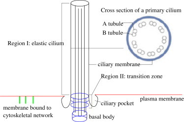
Sketch of the primary cilium structures: Region I is the elastic filament, including both the axoneme and the ciliary membrane. Region II is the transition zone where transition zone fibers connect the transition zone microtubules with the ciliary membrane. Cylindrical geometry is assumed for the transition zone. The cross section of a primary cilium shows the nine pairs of microtubule bundles in the axoneme.
The basal body consists of the mother centriole (with distal and subdistal appendages) and the daughter centriole (see Seeley and Nachury (3) for details). In fact, the basal body is a modified form of the microtubule-organizing center of mitotic spindles. When not involved in mitosis, the mother centriole migrates to the cell membrane, where it is attached to the cell membrane through distal appendages and acts as a template of ciliogenesis and an anchor basal body for the primary cilium. The details of the anchorage are incompletely understood; however, it is known to involve γ-tubulin associated with the basal feet, and unique filamentous structures known as striated rootlets (4).
Between the axoneme and the basal body is a transition zone (TZ), labeled as region II in Fig. 1, where the transition zone fibers (also called ciliary necklace or Y-connectors) bridge the TZ microtubules with the ciliary membrane. These connectors distribute around the TZ microtubules in a more or less symmetrical fashion. As shown in the Fig. 1, the TZ membrane forms a wedge that extends to the ciliary pocket. Adjacent to the ciliary pocket, the membrane is bound to the distal appendages (5,6). The TZ is associated with various proteins and molecular motor transport. It is also found that the lipid composition and the permeability of the TZ membrane are slightly different from that of the ciliary membrane (5,6).
Primary cilia differ from the better-understood motile cilia in several important aspects. For example, primary cilia lack 1), a central pair of microtubule doublet, 2), connections between the outer doublets, and 3), other molecular machinery associated with motility. Unlike motile cilia, there is only one primary cilium per cell. Motile cilia are expressed on specialized cells whereas primary cilia are found on virtually every cell type. Furthermore, primary cilia basal bodies have multiple basal feet and striated rootlets whereas motile cilia have only one of each (7).
Since the initial morphological descriptions of primary cilia over a century ago, their function has only recently begun to be unraveled as a center of chemical and mechanical signal transduction during vertebrate development in bone, kidney, and liver (1). At the beginning, the focus has been on the role of primary cilia in embryonic development where they are known to be involved in establishment of the left-right axis and anterior-posterior limb bud patterning (8–10) via sensing of the Hedgehog and Wnt families of morphogens.
In the kidney cells, Praetorious and Spring (11,12) found a dramatic extracellular calcium-dependent increase in intracellular calcium by bending primary cilia of the epithelial cells with fluid flow or micropipette manipulation. They also verified that this response was lost with removal of primary cilia. It has been suggested that this response occurs via polycystin-2, a cationic channel that localizes to the base of the cilium (13,14). This mechanism has also been found in liver cholangiocytes (15). In addition to its role in flow-sensing, the primary cilium is involved in direct transmission of strains in cartilage extracellular matrix. Mechanosensory function of primary cilia has been suggested in other cell types as well, such as human airway smooth muscle and epithelial cells.
To date, only a handful of articles have been published on theoretical studies of the mechanical behavior of the primary cilium bending under flow. Schwartz et al. (16) developed a mathematical model based on a small-deformation elastic beam formulation. This model assumed a constant velocity and drag profile along the cilium, which was found to break down under high flow conditions. Resnick and Hopfer (17) applied a similar formulation to study small deflections of the primary cilium in a cylindrical Poiseuille flow. Liu et al. (18) used a more precise model of the fluid flow around an array of cilia by numerically solving Stokes equations. They assumed small rotation at the cilium base even though they compute the drag on cilium axoneme consistently from Stokes equations. Rydholm et al. (19) conducted computational fluid dynamics simulations of the bending of an elastic filament connected to an elastic membrane. From their simulations, they found the stress distribution along a filament bent under flow with the maximum stress at the axoneme base. Unfortunately, they did not provide any quantitative comparison of cilium bending under flow between simulations and experiments.
In this article, we conduct a quantitative comparison of cilium bending under flow between experiments and modeling. The mechanics of an elastic beam in a viscous fluid flow is investigated using the slender-body theory (SBT) in the limit of small slenderness
where ϵ ≡ r/L is the ratio of the cross-sectional radius r to the ciliary contour length L. In this limit the nonlocal hydrodynamic interactions are ∼𝒪(β), and the leading-order SBT gives rise to the popular local drag model (20). The local drag model has been widely utilized for studying the dynamics of free actin filaments (21,22) or semiflexible polymers in viscous flow (23). Such leading order SBT is also termed “local SBT” in Tornberg and Shelley (20).
The local drag model is similar to the resistive force theory, which assumes the strength of the singularities is proportional to the local velocity of translation. The main difference lies in the determination of the drag coefficients: In the local SBT, the drag coefficients are determined by the leading-order terms in the SBT formulation (20,24), whereas in the resistive force theory the force coefficients are empirically determined as summarized in Johnson and Brokaw (25).
The (local) SBT allows for large bending of the elastic filament under hydrodynamic load (20,26). In the limit of small filament bending, this model is reduced to those in Schwartz et al. (16) and Resnick and Hopfer (17). Following the formulation in Pozrikidis (27,28), we model the primary cilium as an anchored elastic beam by combining SBT and the model for an elastic beam attached to a wall. The boundary condition for the anchored filament end is determined by how the basal body responds to the hydrodynamic load from the fluid flow. For an equilibrium cilium profile under flow, we assume either clamped or hinged boundary conditions for the basal body by specifying the base angle or curvature, respectively.
Using the cilium base angle from the experiment as a boundary condition for the elastic beam model, we fit the equilibrium cilium profiles to estimate the cilia-bending rigidity EB (= EI, where E is Young’s modulus and I is the moment of inertia of the ciliary axoneme). These equilibrium results uncover the relationship between the total torque and the cilium base angle as a second-order rotational spring. To elucidate the mechanical origin of such a nonlinear rotational spring, we couple the beam-spring system to a cylindrical elastic shell to model the axoneme-membrane system.
The dynamics of the primary cilium toward its equilibrium profile under flow is investigated by integrating our model over time. We further study the tension force distribution along the filament and the elastic shell, and compare it to the critical value for opening a simple mechanosensitive channel, an idealized model for the ion channels that are responsible for the calcium ion transport triggered by bending of primary cilium.
Theory
In the formulation, we ignore the inertia effects and consider the Stokes flow regime for the interaction between the primary cilium and the flow. In addition, the aspect ratio of primary cilia ϵ is often in the range 10−2 ≤ ϵ ≤ 10−1. Consequently, the relevant physics is the bending of an anchored elastic slender filament under fluid flow.
In the model, we need appropriate boundary conditions for the cilium anchorage that correspond to the mechanical responses of the subaxonemal compartment (transition zone, basal body, distal and subdistal appendages, basal feet, and rootlets). Due to the complexity of the subaxonemal compartment, we first model the equilibrium filament attached to a solid wall. For a given hydrodynamic load, we find that the same equilibrium axonemal profiles can be found with either clamped or hinged boundary conditions at the anchored endpoint.
We adopt the elastic beam formulation (27–30) and use the hydrodynamic load from the local drag model. The force distribution is denoted as
with s ∈[s0, se] the arclength, and and the unit tangent and normal vectors, respectively. The curvature κ is assumed to be linearly proportional to the moment M: M = EBκ. The external load is related to the force by
The moment and the force density is related as
Denoting the filament centerline x = (x(s), y(s)) and , the governing equations are
| (1) |
| (2) |
| (3) |
| (4) |
| (5) |
The local filament inextensibility (t1t1s + t2t2s = 0) is utilized in deriving Eqs. 2–4. The dimensionless tangential force and the tension force σ are related as σ = Ft + κ2.
We compute the external load P from the local SBT as
| (6) |
where U is the fluid velocity at the location x in the absence of the elastic filament.
is the effective viscosity with μ the fluid viscosity and the characteristic flow rate. For the equilibrium filament profile, ∂x/∂t = 0 and Eqs. 1–5 can be solved as a set of boundary-value equations with boundary conditions explained as follows.
At the free filament end (s = se), the force-free and torque-free conditions give
| (7) |
At the fixed-end, (s = s0), x(s0) = 0, and y(s0) = 0. If the fixed-end is clamped, the unit tangent vector is specified as
| (8) |
where θ0 is the filament base angle (see Fig. 2). If the fixed-end is hinged with a zero torque, the filament rotates freely and the corresponding boundary conditions are
| (9) |
If there is a localized torque at the filament base (s = s0), the boundary conditions for a hinged filament with a torque at the base are
| (10) |
This can be understood from the equation for the moment M with a localized torque at s0,
| (11) |
where h is the torque magnitude and δ(s = s0) is the Krönecker-delta function at s0. Integrating over a small interval around s0, we find that the localized torque induces a jump in the moment
| (12) |
which, in turn, induces a curvature at the cilium base.
Figure 2.
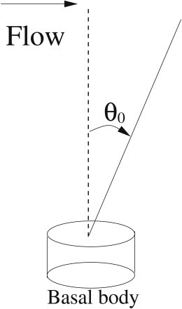
Cilium axoneme coupled to a rotational spring at the cilium base. Under flow the cilium bends, and the basal body support for the basal body is modeled as a rotational spring described by Eq. 18.
For time-dependent filament dynamics, we approximate the time derivative in Eq. 6 by the second-order time discretization
| (13) |
and the equations for the force distribution at the k+1st step are
| (14) |
At every time level, we solve the equations
| (15) |
| (16) |
| (17) |
together with the boundary conditions (see Eq. 7 for the free end and Eqs. 8–10 for the anchored end).
Two more key ingredients need to be incorporated into the formulation based on the following experimental observations:
-
1.Before application of flow the unloaded cilia profiles are often curved, which indicates that there is an internal stress in the axoneme. Such internal stress (denoted as σ0(s)) may be due to the structural change of the axoneme or the basal body (31), and can be included in the constitutive relation as
with σ0(s) determined from the profile of the nonstressed cilium. This can be implemented also in Eq. 17 for the time-dependent model. -
2.The cilium base angle θ0 varies with time as the cilium bends under flow, as shown in Results. This suggests that the fixed angle or curvature assumptions are inappropriate for dynamical modeling. Thus we use a forced overdamped oscillator for the cilium base angle to describe the cilium base rotation
where is the time derivative of θ0. The value f(θ0) is the restoring torque from the basal anchorage, and τ is the torque on the basal body due to the external load on the cilium. At equilibrium and the base angle θ0 can be determined by finding the roots of equation f(θ0) – τ = 0. We determine the functional form of f(θ0) from the experiment. As shown in Results, the restoring torque f(θ0) can be fit by a nonlinear quadratic function.(18)
Table 1 lists the essential parameters in our modeling formulation. Some of the parameters are used later when we couple the elastic filament to a cylindrical elastic shell.
Table 1.
List of parameters
| EB | Bending rigidity of the elastic axoneme |
|---|---|
| η | Effective viscosity (ratio of viscous to elastic forces) |
| ET | Bending rigidity of the cylindrical shell |
| h | Local torque at the transition region |
Materials and Experimental Methods
Materials
Inner medullary collecting-duct kidney (IMCD) epithelial cells with a stable transfection of GFP somatostatin type 3 fusion protein (SSTR-3) were a gift from Professor Brad Yoder (University of Alabama at Birmingham, Birmingham, AL) (32). The cells were cultured in Dulbecco’s modified Eagle’s medium/F12 medium supplemented with 10% fetal bovine serum, 1% penicillin/streptomycin, and 200 μg/mL geneticin G4-18 antibiotic (Invitrogen, Carlsbad, CA). Cells were maintained at 37° and 5% CO2. For flow experiments, cells were seeded at 75,000 cells/mL on a type 1 collagen-coated (33) (BD, Franklin Lakes, NJ) 22 × 44 mm No. 1 coverglass (Warner Instruments, Hamden, CT) and grown to 80–90% confluency. Forty-eight hours before flow and imaging, the cells were serum-starved, then cultured in Dulbecco’s modified Eagle’s medium/F12 medium supplemented with 1% penicillin/streptomycin.
Fluid flow
Fluid shear stress was applied to the IMCD cells in the RC-30 laminar flow chamber (Warner Instruments) by a syringe pump (Kent Scientific, Torrington, CT) with a 30 mL syringe (BD). A quantity of 20 mL of PBS (Invitrogen) was used as the perfusion liquid. The flow chamber had a height H of 250 μm, a width B of 3.2 mm, and a length of 38 mm. The flow rates used ranged between 1 and 3 mL/min and were selected to replicate physiological shear stress conditions (34). Flow was instantaneous and unidirectional for 5 s and was applied once to each slide. Assuming laminar Stokes flow for a parallel-plate flow chamber, the shear stress in the vicinity of the walls for flow between infinitely wide parallel plates depends linearly on the flow rate
where τ is the shear stress, μ is the dynamic viscosity, and Q is the flow rate (35). The flow velocities near the cilia correspond to a 0.4–1.27 Pa wall shear stress. There is some error when calculating the shear forces because the glass slides flex with flow (<15 μm in height). Thus our shear stress estimate is only accurate to within ±0.02 Pa.
Imaging
Two-dimensional xz and three-dimensional xyz image stacks of primary cilia deflecting under fluid flow were captured with a TCS SP5 laser-scanning confocal microscope (Leica Microsystems, Wetzlar, Germany). Images were acquired with a 100×, 1.46 NA oil immersion No. 1 coverglass-aberration-corrected objective, using a 6-kHz resonant bidirectional scanner. The SSTR-3 was expressed along the full length of axoneme, allowing nearly maximum image acquisition of the primary cilium. An Argon laser (488 nm) was used to excite the GFP fusion protein, and the emitted light was collected at 500–600 nm.
Primary cilia were recorded under the fluid flow conditions described above at 10 fps for xz and 4 fps for xyz under 100× optical magnification +10× digital zoom. Cilia were imaged for a total of 2 min: 10 s before the onset of flow (100 frames for xz, 40 frames for xyz), 5 s during the application of flow (50 frames for xz, 20 frames for xyz), and 105 s during the recovery period (1050 frames for xz, 420 frames for xyz). For the equilibrium, cilium profiles xyz image stacks are taken with a z-step size ranging from 0.3 μm to 0.8 μm; this is done because some cilia are shorter than others. For the dynamic data set, the xz plane of the cilium was imaged in profile, and the cilium length measurement is limited by 1), out-of-plane deflection, and 2), the determination of the free end-point. Both limitations lead to variation of cilium length (<0.4 μm) over time.
Before imaging, we ensure that no cilia have experienced fluid flow, and only one primary cilium per slide was recorded during flow. Thirty-five slides were utilized in each experimental group and experiments were repeated three times over multiple days, totaling 105 total cilia imaged. Cells were imaged in the center of the flow chamber to reduce wall effects (35).
Image processing
The image stacks were contrast-enhanced using ImageJ software (National Institutes of Health, Bethesda, MD) and processed with MATLAB (The MathWorks, Natick, MA) to find the xz (two-dimensional) and the xyz (three-dimensional) coordinates of the primary cilium. Images were converted into eight-bit grayscale image and a Gaussian filter was applied to decrease noise before applying a threshold. The x and y components of the sampled pixels were averaged and recorded as the center of the primary cilium. Primary cilium length was calculated manually by first fitting a polynomial curve through the xz or xyz points and then measuring the length between the endpoints. Noise due to magnification and the cilia fluctuating out of the focal plane caused length variations for individual cilia between images. Not all cilia imaged were used, and cilia that significantly moved out of the focal plane were also excluded in the analysis (34). Rotation at the base of the cilium was calculated by fitting a polynomial curve through the first four points of the primary cilium image stack and finding the angle between the curve and the normal (glass coverslip). A total number of 80 primary cilia were analyzed.
Methods of fitting
We used the following procedures to systematically find the least-square fits to the experimentally obtained equilibrium cilium profiles:
-
1.
To begin, we normalize the nonstressed cilium profile before the fluid flow is turned on. The contour length is scaled to unity and the internal stress σ0 is computed from the nonstressed profile.
-
2.
We then normalize the equilibrium cilium profile under a constant flow, and extract the filament angle at the base, θ0, from the normalized data points.
-
3.
Both the internal stress σ0 and the angle θ0 are used to fit a clamped cilium to the normalized cilium profile, and a value of η is obtained from the least-square fit. Fig. 3 shows four sets of experimental data superimposed with their corresponding least-square fits.
Figure 3.
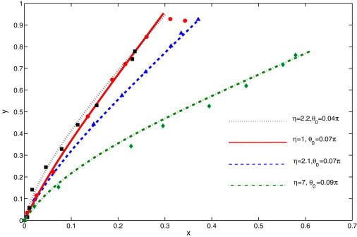
Comparison of filament deflection under shear flow between simulation (curves) and experiment (symbols). The cilium is clamped with a base angle θ0. The value η is found from the least-square fit. (Top to bottom in the legend) Corresponding cilium lengths are 2.1 ± 0.3, 4.7 ± 0.5, 3.6 ± 0.4, and 2.9 ± 0.4 μm and t = 0, respectively.
Results
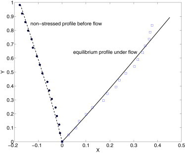
Fig. 4 depicts two xz images of a primary cilium reconstructed from the image stacks. Fig. 4, top, is the cilium before the flow is turned on and Fig. 4, bottom, is the equilibrium profile of the cilium under flow. The statistics of the bending rigidity EB for the whole data set of 80 cilia is summarized in Fig. 5. Almost 70% of the data set falls in the range of 1 ≤ EB ≤ 5 × 10⁻²³ N – m2. The dashed line in the plot indicates the average value, which is higher than reported in Schwartz et al. (16) and lower than recent results in Downs et al. (31). The average cilium length is 3.9 μm with a standard deviation of 0.8 μm over the 80 primary cilia analyzed.
Figure 4.
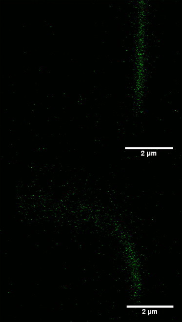
Examples of cilium profiles reconstructed from the xz stacks. (Top) Primary cilium profile before the flow is applied. (Bottom) Equilibrium cilium profile under flow.
Figure 5.
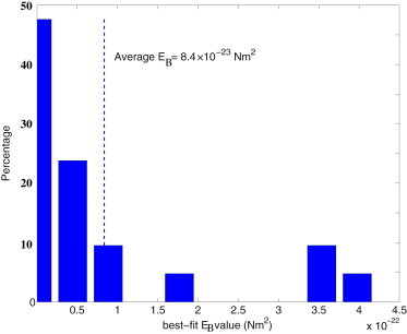
Probability distribution of the estimated axoneme rigidity EB for the primary cilium equilibrium profiles from the experiments.
Combining the cilium base angle (from the experimental data) and total torque (from the least-square fits in our model), we find that the total torque at the base is a nonlinear function of the equilibrium cilium base angle displacement. As shown in Fig. 6, the concave-down dashed line is the least-square quadratic polynomial fit to the full data set (open symbols). The concave-up solid line is the least-square quadratic polynomial fit to the partial data set (solid symbols). Based on the results in Fig. 6, we assume that the equilibrium-restoring torque from the basal body anchorage takes the form
| (19) |
where |b| is proportional to the linear spring constant, and a/b is the relative strength of nonlinearity. At equilibrium, the restoring torque balances with the total torque at the cilium base f(θeq = τ). For the quadratic restoring force in Eq. 19, two equilibrium angles θeq exist for a given τ,
| (20) |
Linear stability analysis on the equilibrium angle θeq shows that θeq is stable for
and unstable for f′(θeq) < 0. This implies that the equilibrium angle along the concave-up solid curve in Fig. 6 is always stable. For the concave-down dashed curve, the equilibrium cilium profile with an angle θeq < 0.3 is stable whereas θeq > 0.3 is unstable. A stable equilibrium angle always exists for θeq < 0.3 for both curves in Fig. 6. Thus, we incorporate the smaller angle in Eq. 20 into the model. With the coefficients (a,b) from either of the fits in Fig. 6, we can determine the cilium base angle for a given torque τ, either during the bending process or for the equilibrium. An example is illustrated in Fig. 7.
Figure 6.
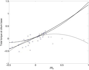
Total torque at cilium base versus the equilibrium cilium angle. Δθ ≡ θeq − θ0 (t = 0) is the equilibrium angle relative to the initial value. (Dashed line) Least-square fit to the full data set (open symbols); (solid line) fit to the partial data set (solid symbols). (Dash-dotted line) From the elastic beam-shell model in Results.
Figure 7.
Fitting the equilibrium cilium profile under flow with the nonstressed cilium profile and nonlinear rotational stiffness. The cilium length is 4.1 ± 0.3 μm.
A nonzero c in Eq. 19 means a nonzero restoring torque is needed when the cilium angle is zero. Nonvanishing c also implies a nonzero base angle when the torque τ = 0. The value of c may be related to the detailed structures of the subaxonemal compartment, and it may be different for different cells. To elucidate the physiological meaning of this constant, we couple the elastic beam to an elastic cylindrical shell as follows.
The elastic shell surface is parameterized as (r(l), z(l)), with l ∈ [l0,le] the arc-length along the elastic sheet. The symbol ψ is the angle between the elastic shell normal vector n and the r axis (see Fig. 8). The governing equations for the cylindrically symmetric elastic incompressible sheet are (36,37)
| (21) |
| (22) |
| (23) |
| (24) |
| (25) |
| (26) |
where ET is the bending rigidity of the transition membrane. In the following we assume that ET ≡ λEB with λ ∼ 𝒪(1). At l = l0 the elastic sheet is connected to the filament, and at l = le it is connected to the surrounding membrane.
Figure 8.
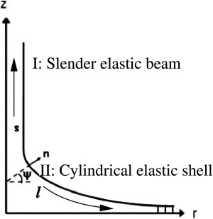
Coordinate system for the cylindrical shell in the transition zone. Region I is the elastic slender beam, and region II is the transition zone that is bound to the distal appendages (small vertical bars on the right end, where ψ = π/2 is fixed.
Equations 21–25 are coupled to Eqs. 1–5 by the boundary conditions at the junction where the filament base (s = s0) is connected to the shell (l = l0).
First, the unit tangent vector is continuous: The filament tangent vector at the base is related to the angle ψ as
Secondly, the force distribution and the curvature are also continuous at the junction
where LS and LB are the characteristic lengths for the shell and beam, respectively.
As explained in Introduction, the TZ fibers connect the TZ microtubules to the membrane. Here we assume that the mechanical support from the basal body can be modeled as a localized finite torque (from the transition fibers) on the elastic cylindrical shell at l = l0. In Theory we show that such a localized torque introduces a jump in the moment at the junction μ(l0) = M(s0) + h, and h/EB is the curvature at the cilium base due to the torque from the TZ fibers.
At the junction the radius of the elastic sheet r(l0) is taken to be the radius of the cilium, and the height of the transition membrane z(l0) is assumed to be of the same order as the filament radius. At the opposite end point, the elastic sheet is assumed to be connected to the cell membrane in a flat angle such that ψ(le) = π/2. Equations 21–25 are rendered dimensionless by scaling the length to the filament radius rf and force to EB/rf2.
In our beam-shell model the torque h signifies the mechanical support from the TZ fibers. Fig. 9 illustrates the cilium-transition zone profiles for different values of h. A nonzero h is needed to support the axoneme in the upright position in the absence of flow because the unforced equilibrium is a flat horizontal shell connected to a horizontal straight beam. As the cilium basal body is mechanically connected to the ciliary membrane through the connectors and microtubular distal appendages, it seems physiologically feasible that nonzero h is related to the support from the transitional fibers that are connected to the ciliary membrane. Numerically we find that the value of h required to support the upright cilium axoneme is proportional to λ, and in dimensionless units h = −0.145 when λ = 1/10 and h = −0.402 when λ = 1/3.6.
Figure 9.
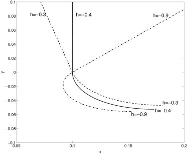
Cilium-transition zone profile in a quiescent flow (η = 0) with different torque h at the base.
The dash-dotted curve in Fig. 6 plots the total torque at the base versus the equilibrium angle with λ = 1/3.6. As discussed in Results, f′(θ) > 0 guarantees a stable equilibrium angle. The concave up-curve from the elastic beam-shell model suggests that the data for large positive equilibrium angles may not be reliable. On the other hand, if these large positive angles are reliable, more biological and mechanical features of the subaxonemal compartment are needed to explain the concave down fit to the nonlinear restoring torque curve (dashed line).
Dynamics toward equilibrium
In physiological situations different timescales may be important, such as the time for the cilium to reach the equilibrium profile under flow and the time for the cilium to relax without external load. These timescales are important for the mechanotransduction processes that primary cilia have been implicated in.
As a first step toward understanding how these dynamical processes are related to mechanosensing, we use our model to simulate the dynamics of cilium bending under flow and cilium relaxation when the flow is turned off. Such dynamical processes can be captured by a high-speed imaging, as shown in Fig. 10 a, where the flow is turned on at t = 0 and the cilium bends as time progresses. In Fig. 10 b, the flow is turned off at t ∼ 5 s and the cilium relaxes to the profile labeled at t = tf ∼ 9.6 s.
Figure 10.
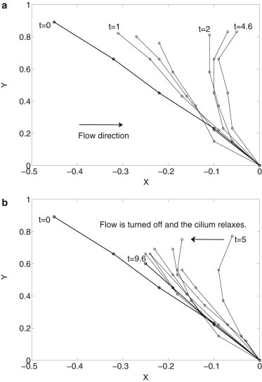
(a) Flow is turned on at t = 0. As time progresses to t ∼ 4.6 s, the cilium bends until it reaches a maximum. (b) The flow is turned off and the cilium relaxes from t = 5 s until reaching a stress-free configuration at t = tf ∼ 9.6 s. The cilium length is 2.7 ± 0.5 μm and t = 0.
The cilium profile data are obtained by high-speed z-stack scanning of the fluorescence proteins on the ciliary membrane. Consequently, noise cannot be estimated and the observed cilium length may not be the same for a single cilium over the duration of 10 s (Fig. 10). In addition, we observe that the initial nonstressed cilium profile in Fig. 10 is not upright. We also note that after the flow is turned off, the cilium does not relax to the original nonstressed profile, as reported in Downs et al. (31).
In our model simulation, we assume that the rotational spring is overdamped. This implies that at any point in time, the cilium base angle is determined by solving f(θ0) – τ|t = 0. Physically this means that we assume the cilium base angle reaches the semiequilibrium value instantaneously as the cilium responds to the hydrodynamic environment. This may be an oversimplification worthy of further investigation.
The comparison between experimental and computational findings is summarized in Fig. 11. The horizontal coordinates of the cilium tip are plotted versus time in Fig. 11 a. The comparison in cilium profile at different times is shown in Fig. 11 b. Symbols are the x-coordinate of the cilium tip in experiment at different times. To compensate the fluctuating cilium length in the experiments, we interpolate or extrapolate the cilium profiles to equal cilium length. The curves are from the simulations. The cilium bends and quickly reaches the maximum bending under flow. The flow is stopped at t ∼ 5 s and the cilium relaxes to a profile close to the initial one. Despite the noises, results indicate that cilium bending and relaxation is well approximated by our simple model incorporating viscous stress, rotational stiffness, and residual stress.
Figure 11.
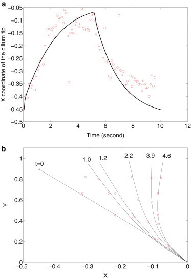
Comparison between model and experiment results shown in Fig. 8. Panel a plots the x-coordinate of cilium tip versus time, and panel b compares the cilium profiles at different times. The cilium length is 2.7 ± 0.5 μm and t = 0.
The relaxation time of the cilium is considerably longer than the elastic relaxation time of a free semiflexible elastic filament (23). This may be understood by taking into account the rotational relaxation time due to the basal body anchorage (such as the shear elastic modulus of the transition membrane due to its coupling with the subaxonemal compartment). However, more of the structural details of the ciliary basal body are needed to fully understand the origin of the rotational relaxation at the base.
Discussion and Conclusion
The bending of the primary cilium due to fluid flow is known to open membrane ion channels. The molecular details of the transmembrane proteins reveal some aspects of their function and behavior. However, little is known about the mechanical coupling between the bending of a primary cilium under flow and the activation of ion channels.
Quantitative description of simple mechanosensitive channels (MscL) in idealized configurations reveals that a critical tension in the lipid bilayer membrane is required to activate an ion channel. By incorporating an ion-channel protein into the free-energy formulation of a planar lipid bilayer membrane, the critical line tension required to keep the protein open can be expressed in terms of the bending rigidity for an individual leaflet, the width of the hydrophobic patch of channel protein, the average size of the ion channel in the open and closed states, and the spring constant for the mismatch between the membrane and protein hydrophobic patch. Once the force in the membrane is large enough to overcome the critical force, MscL will be activated to facilitate the transmembrane transport of ions such as calcium (38–40).
In our calculations, we find that the tension force along the elastic filament and the membrane has a maximum at the junction. The tension force along the cilium is plotted in Fig. 12 a. The corresponding tension force along the transition membrane is shown in Fig. 12 b. The maximum tension on the transition membrane is much smaller than that along the cilium axoneme. This implies that channels on the axoneme near the base are more likely to be open due to the bending under flow.
Figure 12.
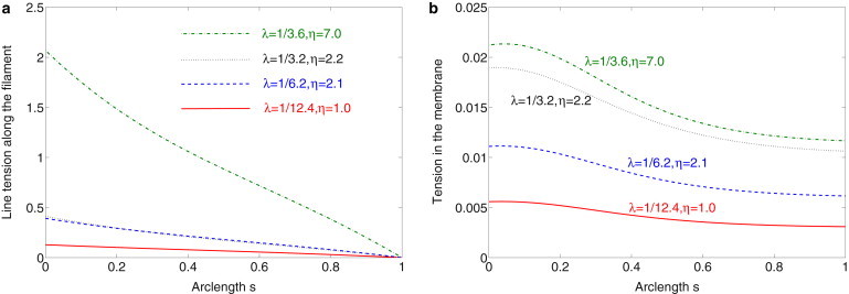
(a) Spatial distribution of the tension force along the cilium with parameters from the fits to the four data sets in Fig. 4. (b) The spatial distribution of the tension force along the membrane with parameters from the fits to the four data sets in Fig. 4.
To compare this tension with the critical tension required to open MscL, we need to know how the axoneme tension is related to the tension along the ciliary membrane. We also note that the critical force for opening MscL is computed based on several assumptions (38–40). The first key assumption is that the reference lipid bilayer membrane profile is assumed to be flat. The second assumption is that mechanical force alone is sufficient to open the transmembrane channel. Finally, the cylindrical symmetry assumed for the transition membrane needs to be relaxed for us to make a refined comparison.
Acknowledgments
Y.N.Y. acknowledges helpful discussion with J.-C. Liao, T. Majmudar, M. Shelley, M. Siegel, and J. Zhang.
Y.N.Y. acknowledges partial support from the National Science Foundation through grants CBET-0853673, DMS-0708977, and DMS-0420590 for the computing cluster at the New Jersey Institute of Technology. C.R.J. is supported by the National Institute of Arthritis and Musculoskeletal and Skin Diseases/National Institutes of Health through grants No. AR45989, No. AR54156, and No. AR62177, and New York State Stem Cell Research grant No. N08G-210.
References
- 1.Bloodgood R.A. From central to rudimentary to primary: the history of an underappreciated organelle whose time has come. The primary cilium. In: Sloboda R.D., editor. Methods in Cell Biology, Vol. 94: Primary Cilia. Academic Press; San Diego, CA: 2009. pp. 3–52. [DOI] [PubMed] [Google Scholar]
- 2.Satir P., Pedersen L.B., Christensen S.T. The primary cilium at a glance. J. Cell Sci. 2010;123:499–503. doi: 10.1242/jcs.050377. [DOI] [PMC free article] [PubMed] [Google Scholar]
- 3.Seeley E.S., Nachury M.V. Constructing and deconstructing roles for the primary cilium in tissue architecture and cancer. In: Sloboda R.D., editor. Methods in Cell Biology, Vol. 94: Primary Cilia. Academic Press; San Diego, CA: 2009. pp. 300–311. [DOI] [PMC free article] [PubMed] [Google Scholar]
- 4.Hagiwara H., Kano A., Ohwada N. Immunocytochemistry of the striated rootlets associated with solitary cilia in human oviductal secretory cells. Histochem. Cell Biol. 2000;114:205–212. doi: 10.1007/s004180000184. [DOI] [PubMed] [Google Scholar]
- 5.Ishikawa H., Marshall W.F. Ciliogenesis: building the cell’s antenna. Nat. Rev. Mol. Cell Biol. 2011;12:222–234. doi: 10.1038/nrm3085. [DOI] [PubMed] [Google Scholar]
- 6.Rohatgi R., Snell W.J. The ciliary membrane. Curr. Opin. Cell Biol. 2010;22:541–546. doi: 10.1016/j.ceb.2010.03.010. [DOI] [PMC free article] [PubMed] [Google Scholar]
- 7.Kwon R.Y., Hoey D.A., Jacobs C.R. Mechanobiology of Primary Cilia. In: Gefen A., editor. Cellular and Biomolecular Mechanics and Mechanobiology. Springer; NJ: 2011. pp. 99–124. [Google Scholar]
- 8.Marszalek J.R., Ruiz-Lozano P., Goldstein L.S. Situs inversus and embryonic ciliary morphogenesis defects in mouse mutants lacking the KIF3A subunit of kinesin-II. Proc. Natl. Acad. Sci. USA. 1999;96:5043–5048. doi: 10.1073/pnas.96.9.5043. [DOI] [PMC free article] [PubMed] [Google Scholar]
- 9.Haycraft C.J., Serra R. Cilia involvement in patterning and maintenance of the skeleton. Curr. Top. Dev. Biol. 2008;85:303–332. doi: 10.1016/S0070-2153(08)00811-9. [DOI] [PMC free article] [PubMed] [Google Scholar]
- 10.Ehlen H.W., Buelens L.A., Vortkamp A. Hedgehog signaling in skeletal development. Birth Defects Res. C Embryo Today. 2006;78:267–279. doi: 10.1002/bdrc.20076. [DOI] [PubMed] [Google Scholar]
- 11.Praetorius H.A., Spring K.R. Bending the MDCK cell primary cilium increases intracellular calcium. J. Membr. Biol. 2001;184:71–79. doi: 10.1007/s00232-001-0075-4. [DOI] [PubMed] [Google Scholar]
- 12.Praetorius H.A., Spring K.R. Removal of the MDCK cell primary cilium abolishes flow sensing. J. Membr. Biol. 2003;191:69–76. doi: 10.1007/s00232-002-1042-4. [DOI] [PubMed] [Google Scholar]
- 13.Arnsdorf E.J., Tummala P., Jacobs C.R. Non-canonical Wnt signaling and N-cadherin related β-catenin signaling play a role in mechanically induced osteogenic cell fate. PLoS ONE. 2009;4:e5388. doi: 10.1371/journal.pone.0005388. [DOI] [PMC free article] [PubMed] [Google Scholar]
- 14.Nauli S.M., Alenghat F.J., Zhou J. Polycystins 1 and 2 mediate mechanosensation in the primary cilium of kidney cells. Nat. Genet. 2003;33:129–137. doi: 10.1038/ng1076. [DOI] [PubMed] [Google Scholar]
- 15.Masyuk A.I., Masyuk T.V., LaRusso N.F. Cholangiocyte cilia detect changes in luminal fluid flow and transmit them into intracellular Ca2+ and cAMP signaling. Gastroenterology. 2006;131:911–920. doi: 10.1053/j.gastro.2006.07.003. [DOI] [PMC free article] [PubMed] [Google Scholar]
- 16.Schwartz E.A., Leonard M.L., Bowser S.S. Analysis and modeling of the primary cilium bending response to fluid shear. Am. J. Physiol. 1997;272:F132–F138. doi: 10.1152/ajprenal.1997.272.1.F132. [DOI] [PubMed] [Google Scholar]
- 17.Resnick A., Hopfer U. Mechanical stimulation of primary cilia. Front. Biosci. 2008;13:1665–1680. doi: 10.2741/2790. [DOI] [PubMed] [Google Scholar]
- 18.Liu W., Murcia N.S., Satlin L.M. Mechanoregulation of intracellular Ca2+ concentration is attenuated in collecting duct of monocilium-impaired Orpk mice. Am. J. Physiol. Renal Physiol. 2005;289:F978–F988. doi: 10.1152/ajprenal.00260.2004. [DOI] [PubMed] [Google Scholar]
- 19.Rydholm S., Zwartz G., Brismar H. Mechanical properties of primary cilia regulate the response to fluid flow. Am. J. Physiol. Renal Physiol. 2010;298:F1096–F1102. doi: 10.1152/ajprenal.00657.2009. [DOI] [PubMed] [Google Scholar]
- 20.Tornberg A.-K., Shelley M.J. Simulating the dynamics and interactions of flexible fibers in stokes flows. J. Comput. Phys. 2004;196:8–40. [Google Scholar]
- 21.Wiggins C.H., Riveline D., Goldstein R.E. Trapping and wiggling: elastohydrodynamics of driven microfilaments. Biophys. J. 1998;74:1043–1060. doi: 10.1016/S0006-3495(98)74029-9. [DOI] [PMC free article] [PubMed] [Google Scholar]
- 22.Wiggins C.H. Biopolymer mechanics: stability, dynamics and statistics. Math. Methods Appl. Sci. 2001;24:1325–1335. [Google Scholar]
- 23.Munk T., Hallatschek O., Frey E. Dynamics of semiflexible polymers in a flow field. Phys. Rev. E Stat. Nonlin. Soft Matter Phys. 2006;74:041911. doi: 10.1103/PhysRevE.74.041911. [DOI] [PubMed] [Google Scholar]
- 24.Pozrikidis C. Oxford University Press; New York: 1997. Introduction to Theoretical and Computational Fluid Dynamics. [Google Scholar]
- 25.Johnson R.E., Brokaw C.J. Flagellar hydrodynamics. A comparison between resistive-force theory and slender-body theory. Biophys. J. 1979;25:113–127. doi: 10.1016/S0006-3495(79)85281-9. [DOI] [PMC free article] [PubMed] [Google Scholar]
- 26.Young Y.-N. Hydrodynamic interactions between two semiflexible inextensible filaments in Stokes flow. Phys. Rev. E. 2009;79:046317. doi: 10.1103/PhysRevE.79.046317. [DOI] [PubMed] [Google Scholar]
- 27.Pozrikidis C. Shear flow over cylindrical rods attached to a substrate. Fluids Struct. 2010;26:393–405. [Google Scholar]
- 28.Pozrikidis C. Shear flow past slender elastic rods attached to a plane. Int. J. Solids Struct. 2011;48:137–143. [Google Scholar]
- 29.Gueron S., Liron N. Ciliary motion modeling, and dynamic multicilia interactions. Biophys. J. 1992;63:1045–1058. doi: 10.1016/S0006-3495(92)81683-1. [DOI] [PMC free article] [PubMed] [Google Scholar]
- 30.Gueron S., Levit-Gurevich K. A three-dimensional model for ciliary motion based on the internal 9+2 structure. Proc. Biol. Sci. 2001;268:599–607. doi: 10.1098/rspb.2000.1396. [DOI] [PMC free article] [PubMed] [Google Scholar]
- 31.Downs M.E., Nguyen A.M., Jacobs C.R. An experimental and computational analysis of primary cilia deflection under fluid flow. Comput. Methods Biomech. Biomed. Engin. 2011 doi: 10.1080/10255842.2011.653784. [DOI] [PMC free article] [PubMed] [Google Scholar]
- 32.Berbari N.F., Johnson A.D., Mykytyn K. Identification of ciliary localization sequences within the third intracellular loop of G protein-coupled receptors. Mol. Biol. Cell. 2008;19:1540–1547. doi: 10.1091/mbc.E07-09-0942. [DOI] [PMC free article] [PubMed] [Google Scholar]
- 33.Ruhfus B., Bauernschmitt H.G., Kinne R.K.H. Properties of a polarized primary culture from rat renal inner medullary collecting duct (IMCD) cells. In Vitro Cell. Dev. Biol. Anim. 1998;34:227–231. doi: 10.1007/s11626-998-0128-4. [DOI] [PubMed] [Google Scholar]
- 34.Donahue T.L.H., Haut T.R., Jacobs C.R. Mechanosensitivity of bone cells to oscillating fluid flow induced shear stress may be modulated by chemotransport. J. Biomech. 2003;36:1363–1371. doi: 10.1016/s0021-9290(03)00118-0. [DOI] [PubMed] [Google Scholar]
- 35.Bacabac R.G., Smit T.H., Klein-Nulend J. Dynamic shear stress in parallel-plate flow chambers. J. Biomech. 2005;38:159–167. doi: 10.1016/j.jbiomech.2004.03.020. [DOI] [PubMed] [Google Scholar]
- 36.Schumacher K.R., Popel A.S., Spector A.A. Modeling the mechanics of tethers pulled from the cochlear outer hair cell membrane. J. Biomech. Eng. 2008;130:031007. doi: 10.1115/1.2907758. [DOI] [PubMed] [Google Scholar]
- 37.Schumacher K.R., Popel A.S., Spector A.A. Computational analysis of the tether-pulling experiment to probe plasma membrane-cytoskeleton interaction in cells. Phys. Rev. E. 2009;80:041905. doi: 10.1103/PhysRevE.80.041905. [DOI] [PMC free article] [PubMed] [Google Scholar]
- 38.Perozo E., Kloda A., Martinac B. Physical principles underlying the transduction of bilayer deformation forces during mechanosensitive channel gating. Nat. Struct. Biol. 2002;9:696–703. doi: 10.1038/nsb827. [DOI] [PubMed] [Google Scholar]
- 39.Wiggins P., Phillips R. Analytic models for mechanotransduction: gating a mechanosensitive channel. Proc. Natl. Acad. Sci. USA. 2004;101:4071–4076. doi: 10.1073/pnas.0307804101. [DOI] [PMC free article] [PubMed] [Google Scholar]
- 40.Phillips R., Kondev J., Theriot J. Garland Science; New York: 2009. Physical Biology of the Cell. [Google Scholar]