Reduced Rank Ridge Regression and Its Kernel Extensions

Abstract

In multivariate linear regression, it is often assumed that the response matrix is intrinsically of lower rank. This could be because of the correlation structure among the prediction variables or the coefficient matrix being lower rank. To accommodate both, we propose a reduced rank ridge regression for multivariate linear regression. Specifically, we combine the ridge penalty with the reduced rank constraint on the coefficient matrix to come up with a computationally straightforward algorithm. Numerical studies indicate that the proposed method consistently outperforms relevant competitors. A novel extension of the proposed method to the reproducing kernel Hilbert space (RKHS) set-up is also developed.

1. INTRODUCTION

Multivariate linear regression is the simple extension of the classical univariate regression model to the case where we have Q > 1 responses and P predictors. It is commonly used in chemometrics, econometrics, and other similar quantitative fields where one is interested in predicting several responses generated by a single production process.

We can express the multivariate linear regression model in matrix notation. Let X denote the N × P predictor or design matrix, with ith row x_i = (x_i1, x_i2, …, x_iP). Similarly the response matrix is denoted by Y, N × Q where the ith row is y_i = (y_i1, y_i2, …, y_iQ). The regression parameter is given by the coefficient matrix B which is P × Q. Note that the qth column of B, β_q = (β_1q, β_2q, …, β_Pq) is the regression coefficient vector for regressing the kth response on the predictors. Let E denote the N × Q random error matrix, then the model is,

$$\mathbf{Y}=\mathbf{XB}+\mathbf{E}.$$ (1)

Note that this will reduce to the classical univariate regression model if Q = 1. For notational simplicity we will assume that the columns of the response and the predictors are centered and scaled so that the intercept terms can be omitted. The most standard approach to estimating the coefficient matrix B is by Ordinary Least Squares approach. The estimator is,

$${\widehat{\mathbf{B}}}_{\text{OLS}}={({\mathbf{X}}^{\text{T}}\mathbf{X})}^{-1}{\mathbf{X}}^{\text{T}}\mathbf{Y}.$$ (2)

This amounts to performing Q separate univariate regression of Y_q ‘s on the predictors. The OLS approach fails to take advantage of any relationship or dependence between the responses, thus performs suboptimally when the true response dimension is <Q. In addition it is well known that this type of estimators perform poorly when the predictor variables are highly correlated.

A large number of methods have been proposed to overcome these deficiencies most of which are based on ideas of dimension reduction and tries to find some underlying latent structure. Popular methods include Principal Component Regression [1], Partial Least Squares [2], Canonical Correlation Analysis [3]. All of these methods can be classified under the larger class of Linear Factor Regression, in which the response Y is regressed against a small number of linearly transformed predictors, often called the factors. The models differ in the way they choose the factors. The estimation proceeds in two steps, transforming the original predictors in the chosen factor space and selecting the number of relevant factors r, often achieved through cross validation. It is easy to see that as r decreases we are able to achieve greater dimensionality reduction.

Another dimensionality reduction approach called Reduced Rank Regression [4–7] minimizes the least squares criterion subject to the constraint rank(B) ≤ r for some r ≤ min{P, Q}. This problem can also be motivated from latent variable regression, where we assume that the Q responses are functions of r underlying latent variables. The solution to the reduced rank regression problem involves projection of the usual OLS estimator to a r-dimensional space that explains the maximum variation in terms of the Frobenius norm. As OLS estimator performs poorly when the predictor variables are highly correlated the performance of the reduced rank estimator is also affected when the predictors are collinear.

Yuan et al. [8] proposed a novel dimension reduction method called Factor Estimation and Selection (FES). They try to minimize the constrained least squares criterion,

$$\widehat{\mathbf{B}}=\underset{\mathbf{B}}{argmin}{\left|\right|\mathbf{Y}-\mathbf{XB}\left|\right|}_F^2+\lambda \sum _{j=1}^{min\{P,Q\}}{\sigma }_j(\mathbf{B}),$$ (3)

where σ_j (B) denotes the j th singular value of B. This constraint encourages sparsity in the singular values of B and hence the solution B̂ is of lower rank. Though motivated from linear factor regression this approach avoids the explicit choice of the factor space by choosing a clever set of basis functions. The optimization problem in Eq. (3) is shown to be equivalent to a second order cone program and the authors use the SDPT3 solver to obtain the solution. SDPT3 can solve conic linear optimization problems over a closed, convex pointed set in a finite-dimensional inner-product space [9]. Unlike reduced rank regression solution this provides a continuous regularization path. But as with the reduced rank regression this method also fails to account for the correlation among the predictor variables. The situations where the singular values of B̂_OLS is a poor approximation to σ_j the FES method may suffer heavily.

To directly exploit the correlation structure between the response variables [10] proposed a method they call the Curds and Whey (CW) procedure. The main idea is to borrow strength from the separate OLS regressions by performing a second round of regression of the responses on the OLS estimates. Intuitively if some responses are heavily correlated then we will be able to obtain a better, more stable predictor by averaging over the corresponding OLS estimates. Notationally, CW predictor takes the form Ỹ = Ŷ_OLSM, where M is a Q × Q shrinkage matrix obtained by the second round of regression. The authors show that the CW procedure has some close connections to the canonical covariate analysis, they also develop an easy to implement GCV type criterion to efficiently perform cross-validatory shrinkage.

Several other penalization approaches have been proposed to improve the performance of least square estimates. Most commonly studied are Ridge regression [11] and LASSO regression [12] in the univariate situation, that is, Q = 1. LASSO is used as a tool for variables selection, specifically suited to the case where the number of predictors p is large but only a few of them actually have some effect on the response variables, more commonly known as the sparse set-up. Ridge regression introduces an ℓ₂ penalty, thus it performs shrinkage to handle the issues caused by collinearity in the predictor variables, rather than dimension reduction. Zou and Hastie [13] proposed the Elastic Net another variable selection method which combines the ℓ₁ and ℓ₂ penalties in an effort to utilize the favorable properties of the LASSO and the Ridge at the same time. Elastic Net achieves dimension reduction while controlling for the correlated predictors thus enjoys a grouping property which is useful in many real life scenario. Turlach et al. [14] proposed the ℓ_∞ penalty on the rows of B to enhance simultaneous variable selection. The method is recommended for model identification rather than prediction because of the bias induced due to the ℓ_∞ penalty. Peng et al. [15] proposed a joint constraint function of the form $C(\mathbf{B})={\lambda }_1{\sum }_{p=1}^P{\sum }_{q=1}^Q\mid {\beta }_{pq}\mid +{\lambda }_2{\sum }_{p=1}^P{\left|\right|{\mathbf{B}}_p\left|\right|}_2$ for the identification of Master Predictors. The first penalty encourages sparsity in B whereas the second penalty shrinks some of the entire rows of B to 0 thus enhancing the selection of the Master Predictors. The model is shown to outperform separate LASSO regressions and leads to highly interpretable estimated models in cancer studies. But this model is not exactly designed for the situation where our underlying assumption is that the Q responses actually live in a lower dimensional space.

In this paper we propose a procedure that combines some of the strengths of the estimators discussed above. The underlying assumption is that the true model is rank deficient, that is, rank(B) ≤ min{P, Q}. Thus the response matrix would approximately be of low rank. Here it is important to note that the response matrix can have approximately low rank when the predictor matrix X is highly collinear even if the true coefficient matrix B is of full rank. We propose a combination of the ridge penalty and rank constraint on the coefficient matrix B to overcome this problem. The ridge penalty helps to ensure that estimate of B is well-behaved even in the presence of multi-collinearity, whereas the rank constraint encourages dimension reduction.

The rest of the paper is organized as follows: In Section 2 we formally introduce the reduced rank ridge regression model and discuss some of the finer details. Section 3 presents numerical examples which include simulation studies comparing the proposed model to relevant competitors as well as some real-data example. We extend the reduced rank approach to the kernel setting in Section 4, and show a real data application. Section 5 concludes with a summary and brief discussion.

2. REDUCED RANK RIDGE REGRESSION MODEL

We propose a regularized estimator for the coefficient matrix B. Two penalties are added to the usual squared error loss. Ridge penalty ensures that the estimator of B is well-behaved even in the presence of collinearity among the predictor variables. Rank constraint encourages dimensionality reduction by restricting the rank of B̂. We seek to minimize,

$$\widehat{\mathbf{B}}(\lambda ,r)=\underset{\{\mathbf{B}:\text{rank}(\mathbf{B})\le r\}}{argmin}{\left|\right|\mathbf{Y}-\mathbf{XB}\left|\right|}_F^2+\lambda {\left|\right|\mathbf{B}\left|\right|}_F^2,$$ (4)

where r ≤ min {P, Q}. ${\left|\right|·\left|\right|}_F^2$ denotes the Frobenius norm for matrices. For each fixed λ we can transform this problem to a Reduced Rank Regression problem on an augmented data set. Define,

$${\mathbf{X}}_{(N+P)\times P}^{\ast }=\left(\begin{array}{c}\mathbf{X}\\ \sqrt{\lambda }\mathbf{I}\end{array}\right),{\mathbf{Y}}_{(N+P)\times Q}^{\ast }=\left(\begin{array}{c}\mathbf{Y}\\ \mathbf{0}\end{array}\right).$$ (5)

Then it is a matter of simple algebra to notice that the minimization problem in Eq. (4) is equivalent to the following reduced rank regression problem:

$$\widehat{\mathbf{B}}(\lambda ,r)=\underset{\{\mathbf{B}:\text{rank}(\mathbf{B})\le r\}}{argmin}{\left|\right|{\mathbf{Y}}^{\ast }-{\mathbf{X}}^{\ast }\mathbf{B}\left|\right|}_F^2.$$ (6)

Now we can use the orthogonal projection property of the OLS estimate to decompose the squared error loss function in two parts, ${\left|\right|{\mathbf{Y}}^{\ast }-{\mathbf{X}}^{\ast }\mathbf{B}\left|\right|}_F^2={\left|\right|{\mathbf{Y}}^{\ast }-{\widehat{\mathbf{Y}}}_R^{\ast }\left|\right|}_F^2+{\left|\right|{\widehat{\mathbf{Y}}}_R^{\ast }-{\mathbf{X}}^{\ast }\mathbf{B}\left|\right|}_F^2$. Here ${\widehat{\mathbf{Y}}}_R^{\ast }={\mathbf{X}}^{\ast }{\widehat{\mathbf{B}}}_R^{\ast }$ denotes the Ridge regression estimate which is also the same as the OLS estimate obtained from the linear model Y^* = X^*B + E^*. Note that the first term does not involve B hence we get the following equivalent form for the minimization problem (6) as,

$$\widehat{\mathbf{B}}(\lambda ,r)=\underset{\{\mathbf{B}:\text{rank}(\mathbf{B})\le r\}}{argmin}{\left|\right|{\widehat{\mathbf{Y}}}_R^{\ast }-{\mathbf{X}}^{\ast }\mathbf{B}\left|\right|}_F^2.$$ (7)

Let us assume that ${\widehat{\mathbf{Y}}}_R^{\ast }={\sum }_{i=1}^{\tau }{\sigma }_i{u}_i{v}_i^T$ gives the singular value decomposition of ${\widehat{\mathbf{Y}}}_R^{\ast }$. σ_i ’s denote the singular values, $\stackrel{u_i}{N\times 1}$and $\stackrel{v_i}{Q\times 1}$ denote the left and right singular vectors of ${\widehat{\mathbf{Y}}}_R^{\ast }$, respectively. τ is the rank of ${\widehat{\mathbf{Y}}}_R^{\ast }$ which is usually going to be Q. Then a fairly elementary result in linear algebra known as the Eckart–Young theorem tells us that the best rank r approximation to ${\widehat{\mathbf{Y}}}_R^{\ast }$ in the Frobenius norm is given by,

$${\widehat{\mathbf{Y}}}_r^{\ast }=\sum _{i=1}^r{\sigma }_i{u}_i{v}_i^{\text{T}}.$$ (8)

Define, $\underset{q\times q}{{\mathbf{P}}_r}={\sum }_{i=1}^r{v}_i{v}_i^{\text{T}}$, and let $\widehat{\mathbf{B}}(\lambda ,r)={\widehat{\mathbf{B}}}_R^{\ast }{\mathbf{P}}_r$. Clearly rank (B̂(λ, r)) ≤ r, as rank(P_r) = r. And plugging them back in we get,

$$\begin{array}{l}{\mathbf{X}}^{\ast }\widehat{\mathbf{B}}(\lambda ,r)={\mathbf{X}}^{\ast }{\widehat{\mathbf{B}}}_R^{\ast }{\mathbf{P}}_r=\left(\sum _{i=1}^{\tau }{\sigma }_i{u}_i{v}_i^T\right)\left(\sum _{j=1}^r{v}_j{v}_j^T\right)\\ =\sum _{i=1}^r{\sigma }_i{u}_i{v}_i^T={\widehat{\mathbf{Y}}}_r^{\ast }\end{array}$$

Hence we are able to show that the proposed solution $\widehat{\mathbf{B}}(\lambda ,r)={\widehat{\mathbf{B}}}_R^{\ast }{\mathbf{P}}_r$ is the minimizer of the optimization problem (4), which is the original reduced rank ridge regression problem that we started with. Writing down explicitly in terms of X, Y, λ and r we get the following:

$$\begin{array}{l}\widehat{\mathbf{B}}(\lambda ,r)={\widehat{\mathbf{B}}}_R^{\ast }{\mathbf{P}}_r={({\mathbf{X}}^{\ast \text{T}}{\mathbf{X}}^{\ast })}^{-1}{\mathbf{X}}^{\ast \text{T}}{\mathbf{YP}}_r\\ ={({\mathbf{X}}^{\text{T}}\mathbf{X}+\lambda \mathbf{I})}^{-1}{\mathbf{X}}^{\text{T}}{\mathbf{YP}}_r,\end{array}$$ (9)

$$\widehat{\mathbf{Y}}(\lambda ,r)=\mathbf{X}{({\mathbf{X}}^{\text{T}}\mathbf{X}+\lambda \mathbf{I})}^{-1}{\mathbf{X}}^{\text{T}}{\mathbf{YP}}_r={\widehat{\mathbf{Y}}}_{\lambda }{\mathbf{P}}_r.$$ (10)

Ŷ_λ in the above equation denotes the multivariate ridge regression estimator for Y with a penalty parameter λ. This shows that the reduced rank ridge regression is actually projecting Ŷ_λ to a r-dimensional space with projection matrix P_r. Here it is important to notice that this is a projection of the rows of Ŷ_λ which in general lives in a Q-dimensional space to a lower r-dimensional space. Easy to see that for r = Q we get back the ridge regression solution.

2.1. Illustrative Example

To illustrate the issues with Reduced Rank regression we construct a simple toy example. Set P = Q = 3 and N = 50 and let,

$$\mathbf{B}=\left(\begin{array}{ccc}1& 3& 0\\ 3& 1& 0\\ 0& 0& 0\end{array}\right),{\mathbf{\sum }}_X=\left(\begin{array}{ccc}1& 0.95& 0\\ 0.95& 1& 0\\ 0& 0& 1\end{array}\right).$$

The first two columns of B are linearly independent and thus it has rank 2. But at the same time we make predictors X₁ and X₂ highly collinear, so that the effective dimension of the response reduces to 1. We simulate X ~ N(0, Σ_X) and given X, Y is generated from Y ~ N(XB, 0.25I). The eigenvalues of Y^TY comes out to be σ² = [1252, 16, 11]. Hence Reduced Rank regression would select rank to be 1 and seek a rank 1 estimator of B which is clearly not the case here. This happens because Reduced Rank regression fails to account for the correlation among predictors and that is precisely where Reduced Rank Ridge regression improves by adding ridge penalty.

2.2. Selection of Tuning Parameters

For the reduced rank ridge regression we propose to choose the tuning parameters (λ, r) using a simple K-fold cross-validation procedure. We first define a grid for (λ, r) note that r can only take values in {1, 2, … min {P, Q}}. For each combination of λ and r we evaluate average of validation prediction errors over the K-folds and choose the optimal combination as the one that minimizes this quantity. Notationally,

$$(\widehat{\lambda },\widehat{r})=\underset{\lambda ,r}{argmin}\sum _{k=1}^K{\left|\right|{\mathbf{Y}}^{(k)}-{\mathbf{X}}^{(k)}{\widehat{\mathbf{B}}}^{(-k)}(\lambda ,r)\left|\right|}_F^2,$$ (11)

where X^(k) and Y^(k) denote the predictor and response matrix for the kth fold, and B̂^(−k)(λ, r) denotes the estimated regression coefficient matrix computed leaving out the observations in the kth fold when using the penalty parameters (λ, r). This would encourage a tradeoff between the penalty parameters based on the data. We would look into the choice of tuning parameters more deeply in the simulation studies section.

3. NUMERICAL EXAMPLES

3.1. Simulation Study

We compare the estimation performance of the proposed reduced rank ridge regression method to other multivariate linear regression methods that have been proposed in the literature based on the idea of dimension reduction and borrowing strength from dependent response variables. Methods compared include—Ordinary least square (OLS); Curd and Whey (CW) procedure developed by Breiman and Friedman with the GCV approach; Reduced Rank Regression (RRR); Multivariate Ridge Regression (MVR) with same tuning parameter for each response; Separate Ridge Regression (SR); Partial Least Square (PLS); Principal Component Regression (PCR) and the proposed Reduced Rank Ridge Regression (RRR). For the methods that require a selection of tuning parameter we do so by looking at the prediction error on an independently generated validation set of same size. We measure the performance of various methods by model error following [10]. The model error of an estimate B̂ is given by,

$$\text{ME}(\widehat{\mathbf{B}})=\text{trace}\left[{(\mathbf{B}-\widehat{\mathbf{B}})}^{\text{T}}{\mathbf{\sum }}_X(\mathbf{B}-\widehat{\mathbf{B}})\right],$$ (12)

where B denotes the true coefficient matrix and Σ_X denotes (XX^T).

3.1.1. Models

In each replication of the simulation study we generate a design matrix X_N×P with each rows drawn independently from N(0, Σ_X). Where Σ_X has the structure, Σ_X(i, j) = ρ^|i−j|. We used three different levels for the correlation parameter ρ = [0, 0.5, 0.9]. To generate the true coefficient matrix B_P×Q we first generate a random P × Q matrix from N(0, 1) distribution. The singular values are then replaced with following structures:

• Model 1 The first half of the singular values are 2 and rest as 0.

• Model 2 All the singular values are equal to 1.

• Model 3 The largest singular value as 5 and rest 0.

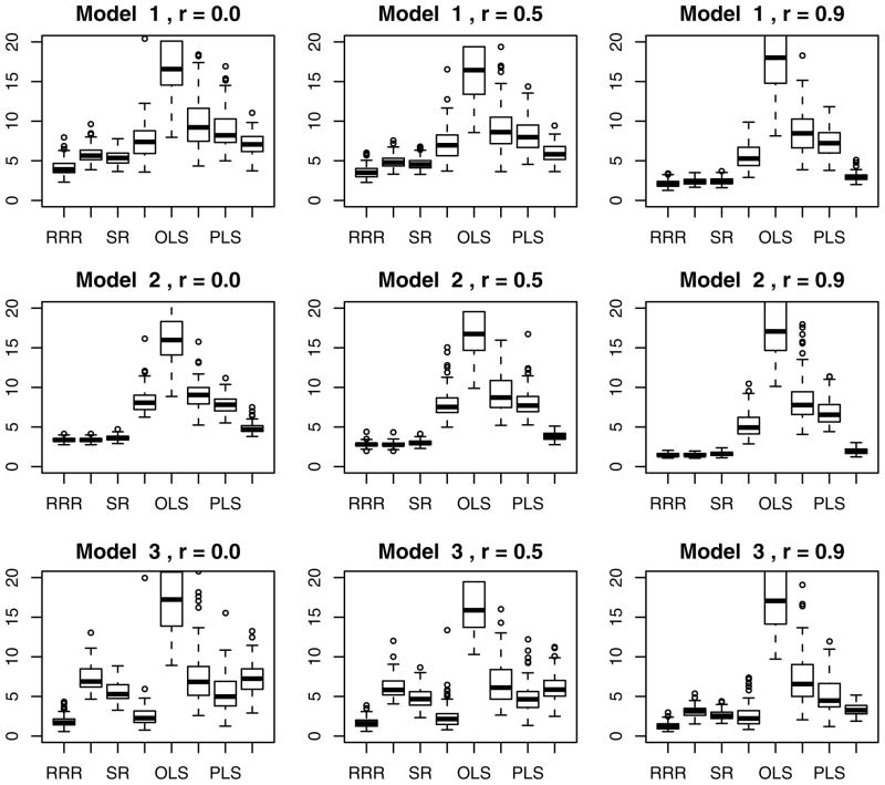
We choose the above mentioned models to ensure that we cover a broad spectrum of rank-deficient situations. Model 2 covers the case of no rank redundancy in the coefficient matrix B which is the usual multivariate linear regression assumption. Model 3 represents the case for a severe rank deficiency, whereas Model 1 is a compromise between these two extreme situations. We analyze each model at different correlation levels between the predictors thus covering most of the possible real scenarios. For each combination of model and correlation we simulate a training and validation set each of size P = 50, Q = 20, N = 100. And compute each of the estimators described above. The process is repeated 100 times leading to an error-vector of length 100 for each competing method (Fig. 1).

Fig. 1.

Boxplot of ME of each method over 100 replicates under each combination of settings.

All the methods outperforms OLS by a big margin under this settings. PLS and PCR appear quite competitive to RR but fails to perform in the same level as RRR, MVR, or SRR. Note that the proposed method RRR dominates all the other methods at every combination of settings. It is interesting to note that for Model 2 where the true B had full rank RR does significantly worse than RRR, MVR, and SRR for all choices of ρ. Whereas in Model 3 which had the strongest rank deficiency we see that RRR and RR dominates the other methods which also seems intuitive. The biggest advantage of the RRR over only ridge and only rank penalty comes in Model 1 which has nearly half the singular values nonzero. For all three models we see that as the value of ρ increases MVR and SRR tends to catch up with the best method.

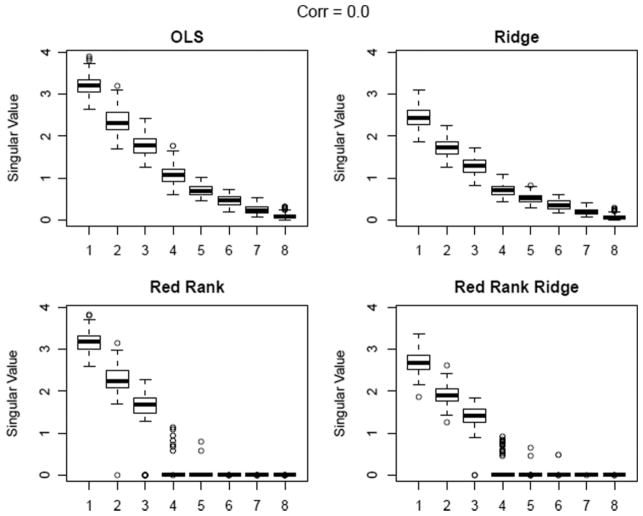
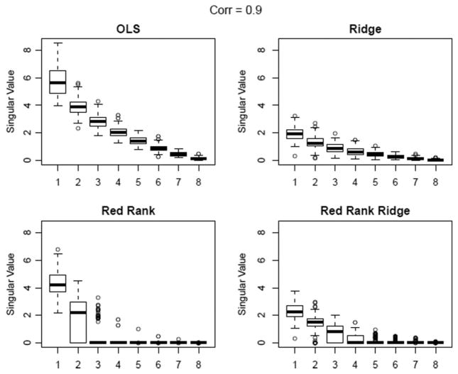
To gain further insight, we look at the singular values of the B̂ for OLS, MVR, RR, and RRR method. For this part we use a smaller set-up with P = 20, Q = 8, and N = 30 the singular values of B are σ = [3, 2, 1.5, 0, 0, 0, 0, 0]. We plot the singular values over 100 replicates at two extreme correlation levels ρ = 0.0, and 0.9 (Figs 2 and 3).

Fig. 2.

Singular values of B̂, ρ = 0.0.

Fig. 3.

Singular values of B̂, ρ = 0.9.

For ρ = 0 we see that both RR and RRR does a fairly good job of recovering the singular value structure. But as the collinearity among the predictors increases we find that RR most of the times selects 2 or 1 as the rank whereas RRR is able to do a much better job. MVR and OLS fail to achieve any dimension reduction. Similar patterns are observed at other settings as well which we skip for brevity. This clearly illustrates that the trade-off between ridge penalty and the rank constraint is the key that enables us to correctly estimate singular value structure even in presence of serious collinearity.

3.2. Application in Chemometrics Example

It is originally from ref. [16]. There are N = 56 observations with P = 22 and Q = 6. The data is generated from a simulation of a low density tubular polyethylene reactor. The predictor variables consist of 20 temperature measurements at equal distance along the reactor along with the wall temperature and the feed rate. The responses are output characteristics of the polymers produced, namely, number avg. molecular weight (Y₁), weight avg. molecular weight (Y₂), long chain branching (Y₃), short chain branching (Y₄), content of vinyl group (Y₅), and content of vinyledene group (Y₆). As the responses were all right skewed we applied log transformation, and finally standardized them. The response correlation matrix is as follows:

$$\text{Corr}(Y)=\left(\begin{array}{rrrrrr}1.00& 0.96& 0.06& 0.25& 0.26& 0.26\\ 0.96& 1.00& -0.13& 0.28& 0.27& 0.28\\ 0.06& -0.13& 1.00& -0.50& -0.48& -0.48\\ 0.25& 0.28& -0.50& 1.00& 0.97& 0.98\\ 0.26& 0.27& -0.48& 0.97& 1.00& 0.98\\ 0.26& 0.28& -0.48& 0.98& 0.98& 1.00\end{array}\right).$$

This shows {Y₄, Y₅, Y₆} form a strongly correlated group as does {Y₁, Y₂}. Y₃ is mildly correlated to the others, which suggests an effective response dimensionality of 3. Average absolute correlation between the predictors is about 0.44 with many of them being very highly correlated. The predictive performance is measured using leave-one-out cross validation. We fit the models based on 55 of the 56 points and predict the left-out point and the procedure is repeated 56 times. Note that we do an 11-fold cross validation within the 55 points to select tuning parameters for the models that have one. We report the prediction error for each response as well as overall average prediction error (Table 1).

Table 1.

Performance comparison for the Chemometrics data.

	OLS	CW-gcv	PLS	RR	MVR	RRR
Y1	0.49	0.49	0.68	0.44	0.15	0.15
Y2	1.12	0.74	0.90	0.46	0.22	0.22
Y3	0.53	0.49	0.45	0.65	0.39	0.39
Y4	0.24	0.18	0.18	0.14	0.26	0.24
Y5	0.30	0.22	0.26	0.18	0.28	0.27
Y6	0.28	0.21	0.21	0.16	0.28	0.27
Avg.	0.50	0.39	0.45	0.34	0.27	0.26

Overall RRR performs the best with MVR being a very close second. The good performance of MVR can also be explained by the fact that many predictors are highly collinear. Comparing columns of RR and RRR, we see that for Y₄, Y₅, and Y₆ RR has much smaller prediction error than RRR but it incurs larger error for Y₁, Y₂ and especially Y₃. Because of the strong correlation structure of the responses, RR concentrates on the heavily correlated group {Y₄, Y₅, Y₆}, selecting 2 or 1 components most times (out of 56 leave-one-out runs) whereas RRR is able to pick 3 as the optimal dimension with high proportion. So even though it loses a little bit for the highly correlated group overall prediction accuracy is much better.

4. EXTENSION TO RKHS

Before we go into the details for reduced rank approach in the Reproducing Kernel Hilbet Space (RKHS) setting let us first give a very brief introduction to it.

4.1. Brief Introduction to RKHS

A Hilbert space is a real/complex inner-product space which is complete under the norm induced by the inner product. Examples include ℝⁿ with 〈x, y〉 = x^Ty, -space of all square functions that can integrate on ℝ with 〈f, g〉 = ∫_ℝf (x)g(x)dx. The reason we are interested in functional spaces is because we would like to fit models like y = f (x) + ε where f : ℝ^p → ℝ to model the data in a much more flexible nonparametric way. is too big for our purpose as it contains too many nonsmooth functions. One way to obtain such spaces of smooth functions which allows us to fit a nonparametric functional regression model without explicitly specifying the function f is the RKHS approach.

A positive definite kernel is a function K(·,·) : × ↦ ℝ such that for any N ≥ 1 and {x₁, x₂, … x_N} ∈ and {a₁, a₂, …, a_N}∈ ℝ^N, we have, ${\sum }_{i=1}^N{\sum }_{i^{\prime }=1}^N{a}_i{a}_{i^{\prime }}K(x_i,x_{i^{\prime }})\ge 0$. In other words the gram matrix $\mathbf{K}={[K(x_i,x_{i^{\prime }})]}_{i,i^{\prime }=1}^N$ is positive definite for all, {x₁, x₂, … x_N} ∈ . For most of our purposes = ℝ^P, the space of the predictor variables. It is well known [17] that given such a kernel we can construct a unique functional Hilbert space on such that K(·,·) is the inner product in that space and f (x) = 〈f, K(·, x)〉 for all f ∈ and x ∈ and vice versa.

4.2. Kernel Reduced Rank Regression Approach

In the univariate case, given data {(x₁, y₁), (x₂, y₂), … (x_N, y_N)}, note that y_i ∈ ℝ and x_i ∈ ℝ^P, our objective is to find a function f ∈ that minimizes,

$$J_{\lambda }(f)=\sum _{i=1}^N{(y_i-f(x_i))}^2+\lambda {\left|\right|f\left|\right|}_{\mathcal{H}}^2,$$ (13)

where ${\left|\right|·\left|\right|}_{\mathcal{H}}^2$ denotes the norm in . This is introduced to encourage smoothness and to avoid overfitting. Then the Representer Theorem says that any f minimizing (13) can be written as,

$$f(x)=\sum _{i=1}^N{\alpha }_{i}K(x,x_i),\text{for}({\alpha }_1,{\alpha }_2,\dots ,{\alpha }_N)\in {\mathbb{R}}^N.$$ (14)

For the multivariate response y_i ∈ ℝ^Q, in the RKHS set-up we want to find (f₁, f₂, …, f_Q) ∈ which minimizes a joint loss function defined as,

$$J_{\lambda }(f_1,f_2,\dots ,f_Q)=\sum _{q=1}^Q\sum _{i=1}^N{\left|\right|y_{iq}-f_q(x_i)\left|\right|}^2+\lambda \sum _{q=1}^Q{\left|\right|f_q\left|\right|}_{\mathcal{H}}^2.$$ (15)

Like in the linear case it is fairly easy to see that in absence of any constraint on the functions (f₁, f₂, …, f_Q) the above optimization is same as doing Q separate single-response kernel ridge regression problem. If we want to exploit the dependence among the responses we need some equivalent way of expressing the reduced rank constraint under the RKHS set-up. The following proposition gives one such way,

PROPOSITION 1

Let be the RKHS corresponding to a positive-definite kernel K(·,·) : ℝ^P × ℝ^P ↦ ℝ. Given data {(x₁, y₁), (x₂, y₂), … (x_N, y_N)}, y_i ∈ ℝ^Q and x_i ∈ ℝ^P, we consider the optimization problem,

$$\underset{f_1,f_2,\dots ,f_Q\in \mathcal{H}}{min}{J}_{\lambda }(f_1,f_2,\dots ,f_Q)\text{subject}\text{to}\text{dim}(\text{span}\{f_1,f_2,\dots ,f_Q\})\le r,$$ (16)

where 1 ≤ r ≤ Q and J_λ (f₁, f₂, …, f_Q) is defined as in Eq. (15). The solution has the following representation,

$$f_q(x)=\sum _{i=1}^N{\alpha }_{iq}K(x,x_i),\text{for}q=1,2,\dots ,Q,{\alpha }_{iq}\in \mathbb{R}.$$ (17)

The constraint dim (span{f₁, …, f_Q} ≤ r can be viewed as an extension to the rank constraint for linear functions. The only difference being instead of working with linear functions here we are in a general functional space. We defer the proof to the appendix.

The next natural step is to find some sufficient conditions under which the rank constraint of Eq. (16) becomes equivalent to a rank constraint on the coefficient matrix A = [α_iq]_N×Q, because that would allow us to extend the reduced rank ridge regression solution developed in Section 2 in a natural way to the kernel setting.

PROPOSITION 2

If K(·,·) is strictly positive definite and {x₁, x₂, … x_N} are distinct then

$$\begin{array}{l}dim(\text{span}\{f_1,f_2,\dots f_Q\})\le r\Rightarrow \text{rank}(\mathbf{A})\le r,\\ \text{where},[f_1,\dots f_Q]=[K(·,x_1),\dots K(·,x_N)]\underset{N\times Q}{\mathbf{A}}.\end{array}$$

This proposition translates the reduced rank constraint for RKHS into a simple rank constraint for the coefficient matrix A, under some condition on K(·,·). It is easy to show that Gaussian kernel, $K(x,x^{\prime })=exp(\frac{-{\left|\right|x-x^{\prime }\left|\right|}^2}{2{\sigma }^2})$, Laplacian kernel, $K(x,x^{\prime })=exp(\frac{{\left|\right|x,x^{\prime }\left|\right|}_1}{2{\sigma }^2})$, Inverse multiquadratic kernel $K(x,x^{\prime })=\frac{1}{\sqrt{{\left|\right|x-y\left|\right|}^2+c}}$ would satisfy strict positive definiteness. Polynomial kernels in general would not satisfy it because it is essentially an extension to a bigger but finite-dimensional space. But in practice the infinite-dimensional RKHS’s are the ones that we would be interested in, so the condition for strict positive definiteness is not very prohibitive.

4.3. Extending the Solution

Let us recall the solution to the reduced rank ridge regression problem with penalty parameters (λ, r), derived in Section 2. For a given point x ∈ ℝ^Q (row vector) prediction had the form,

$${\widehat{Y}}_x(\lambda ,r)=x{({\mathbf{X}}^{\text{T}}\mathbf{X}+\lambda \mathbf{I})}^{-1}{\mathbf{X}}^{\text{T}}{\mathbf{YP}}_r,$$

where P_r was the projection matrix to the space spanned by r principal eigenvectors of P = Y^TX (X^TX + λI)⁻¹ X^TY. Using the matrix inversion lemma we can easily expand the prediction formula in terms of the inner-product matrix XX^T. Then replacing the inner-product matrix by the Gram matrix $\mathbf{K}=[{(K(x_i,x_{i^{\prime }})]}_{i,i^{\prime }=1}^N$ we get,

$${\mathbf{Y}}^{\text{T}}\mathbf{X}{({\mathbf{X}}^{\text{T}}\mathbf{X}+\lambda \mathbf{I})}^{-1}{\mathbf{X}}^{\text{T}}\mathbf{Y}={\mathbf{Y}}^{\text{T}}\mathbf{K}{(\mathbf{K}+\lambda \mathbf{I})}^{-1}\mathbf{Y}$$ (18)

$$x{({\mathbf{X}}^{\text{T}}\mathbf{X}+\lambda \mathbf{I})}^{-1}{\mathbf{X}}^{\text{T}}\mathbf{Y}=K(x){(\mathbf{K}+\lambda \mathbf{I})}^{-1}\mathbf{Y}.$$ (19)

Note that K(x) = [K(x, x₁), K(x, x₂), … K(x, x_N)]_1×N. If we denote the projection matrix to the space spanned by r principal eigenvectors of Y^TK (K + λI)⁻¹ Y by ${\mathbf{P}}_r^K$ then the final prediction for the point x ∈ ℝ^P is given by,

$${\widehat{Y}}_x(\lambda ,r)=K(x){(\mathbf{K}+\lambda \mathbf{I})}^{-1}\mathbf{Y}{\mathbf{P}}_r^K,$$ (20)

which is similar to projection of the kernel ridge regression estimator to a constrained space of dimension ≤r as in the linear case.

4.4. Simulation Study

In this section we compare the performance of the proposed kernel Reduced Rank Ridge Regression (kernel RRR) with kernel Ridge Regression. We perform the comparison with the choice of two popular choices of kernel function namely, the Gaussian kernel which is strictly positive-definite and thus satisfies the condition of Proposition 2 and the polynomial kernel which is clearly finite-dimensional and hence does not satisfy the sufficient condition provided in Proposition 2.

We present the results for P = 10, Q = 10, and N = 100, similar results were obtained for other choices of P and Q. Rows of the design matrix X were generated independently from N(0, I_P). Responses are generated as linear combinations of m = 10 basis functions of the form K(·, b_j) where {b_j : j = 1, 2, …, 10} were generated independently from a multivariate Gaussian distribution. We consider two cases,

• Full Rank Situation: The coefficient matrix is full-rank, that is, of rank 10.

• Reduced Rank Situation The coefficient matrix has rank 5.

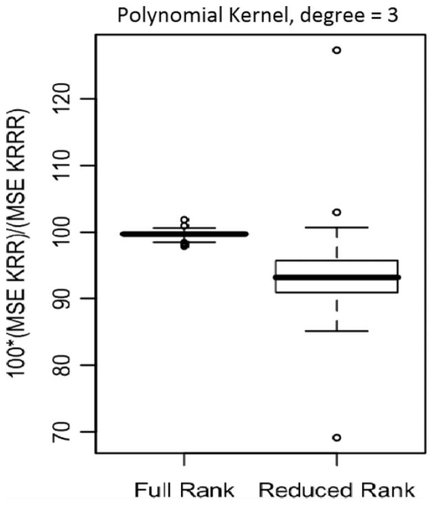
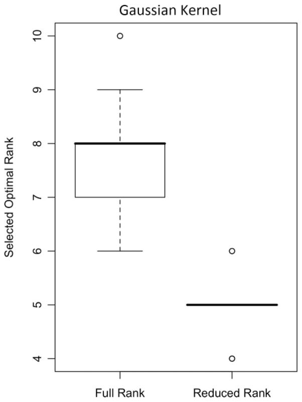
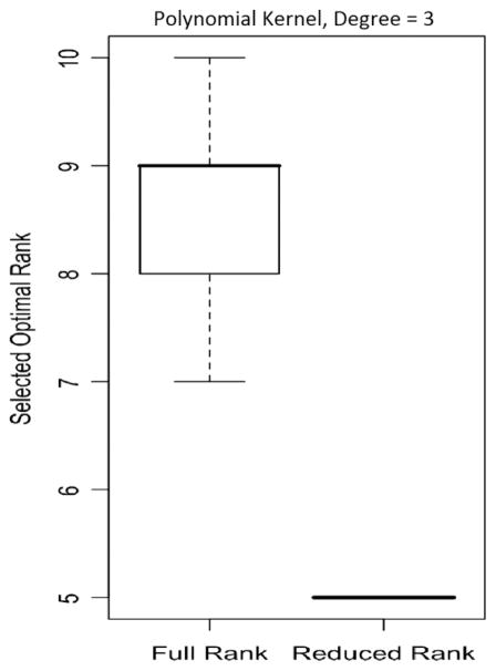
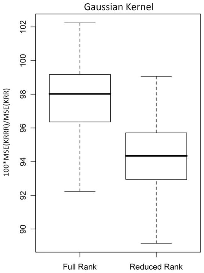
The tuning parameters, that is, (λ, r, s) were chosen using independently generated validation data sets of same size. In Figs 4–7 we present the box-plots of the percentage ratio of MSE of kernel RRR and kernel Ridge Regression over 100 replications of the experiment.

Fig. 4.

Polynomial kernel, % of MSE compared to kernel ridge regression.

Fig. 7.

Gaussian kernel, Box plot of the estimated rank over 100 replications.

As expected we find that kernel Reduced Rank Ridge improves over kernel Ridge significantly when the underlying process is truly low-rank, and even in the full-rank case it performs comparably with kernel Ridge regression. The conclusions hold not only for the Gaussian kernel but for the polynomial kernel as well which as we discussed before does not satisfy the sufficient conditions in Proposition 2. Also the estimated optimal rank seems to be quite accurate when the underlying functional space is low-rank. Here it is useful to note that if the sample size is too high then the gram matrix for polynomial kernel might become nearly singular causing unstable solutions.

4.5. Chemometrics Data Revisited

We apply the kernel RRR on the previously discussed Chemometrics data set and compare its performance against linear RRR and kernel Ridge Regression. We used the popular Gaussian kernel $K(x,x^{\prime })=exp\left(\frac{-{\left|\right|x-x^{\prime }\left|\right|}^2}{2{\sigma }^2}\right)$ and the Inverse multiquadratic kernel $K(x,x^{\prime })=\frac{1}{\sqrt{{\left|\right|x-y\left|\right|}^2+c}}$. Both predictors and responses were standardized for this analysis. An eight fold-cross-validation is performed to select the tuning parameters, that is (λ, r, σ²) in case of the Gaussian kernel and (λ, r, c) for the inverse multiquadratic kernel (Table 2).

Table 2.

Performance comparison for Kernel RRR and Kernel RR for the Chemometrics data with Gaussian and Inverse multi-quadratic kernels.

	Linear RRR	Gaussian Kernel		Inverse multiquadratic Kernel
		Kernel Ridge	Kernel RRR	Kernel Ridge	Kernel RRR
Y1	0.153	0.088	0.087	0.111	0.120
Y2	0.250	0.148	0.129	0.224	0.210
Y3	0.230	0.113	0.111	0.160	0.161
Y4	0.188	0.054	0.044	0.098	0.094
Y5	0.205	0.107	0.071	0.125	0.101
Y6	0.211	0.070	0.064	0.092	0.097
Avg.	0.206	0.097	0.084	0.135	0.131

We used cross-validation error estimate on the hold-out fold to select the tuning parameters. Optimal rank for the kernel RRR which turns out to be 3 for both choices of the kernels as it was for linear Reduced Rank regression implying that the intrinsic dimensionality of the response space is 3. Both choices of the kernel lead to very similar results. Kernel RRR improves by a big margin over the linear RRR, whereas the improvement over kernel ridge regression is less pronounced but still notable for this data set. The Gaussian kernel is able to attain a greater reduction in MSE which is due to the fact that it corresponds to a bigger functional class. The results seem scientifically reasonable since the first two responses namely, number avg. molecular weight and weight avg. molecular weight are approximately dependent. Similarly the last three responses form a functional group, in the sense that, short chain branching is an approximate measure of the contents of Vinyl and Vinyledene groups and thus are highly correlated. Long chain branching is negatively correlated to the short chain branching group.

5. SUMMARY AND DISCUSSION

We propose Reduced Rank Ridge Regression to produce a low-rank estimator of the regression coefficient matrix B. This is very useful when the responses are highly dependent or there are reasons to believe a latent variable structure among the predictors. Our method accounts for multi-collinearity in predictor variables by incorporating a ridge penalty, here it is important to note that both high collinearity in X and low-rank of the true coefficient matrix B might lead to the response matrix being rank-deficient and hence it makes sense to apply the penalties jointly and decide the trade-off based on the data. We also extend the reduced rank idea to the RKHS set-up and give some intuition for the meaning of a rank constraint in a functional space.

The solution to the Reduced Rank Ridge Regression problem is obtained as a projection of the Ridge Regression estimator to a constrained space. And hence it is computationally simple. We propose a cross-validation approach to select the tuning parameters. The proposed method was tested in broad variety of simulation settings as well as couple of real data sets. Results are promising and the proposed method is able to outperform relevant competitors under most of the settings. We also apply the kernel RRR on a real data example and it shows some significant improvement over the linear RRR and kernel ridge regression. These applications also help us understand some statistical insights into the working of the proposed Reduced Rank Ridge Regression method.

Fig. 5.

Polynomial kernel, Box plot of the estimated rank over 100 replications.

Fig. 6.

Gaussian kernel, % of MSE compared to kernel ridge regression.

APPENDIX

Proof of Proposition 1

Let (f₁, f₂, …, f_Q) be the minimizer to Eq. (16). Define,

$${\mathcal{F}}_K=\text{span}\{K(·,x_i):i=1,2,\dots N\}.$$ (21)

We can decompose each $f_q=f_q^{\ast }+f_q^0$ where $f_q^{\ast }$ is the projection of f_q onto and $f_q^0$ is the orthogonal to . Then for j = 1, 2, … Q and i = 1, 2, …, N,

$$\begin{array}{l}{f}_q(x_i)=\langle f_q^{\ast }+f_q^0,K(·,x_i)\rangle =f_q^{\ast }(x_i),\\ {\left|\right|f_q\left|\right|}_{\mathcal{H}}^2={\left|\right|f_q^{\ast }\left|\right|}_{\mathcal{H}}^2+{\left|\right|f_q^0\left|\right|}_{\mathcal{H}}^2.\end{array}$$

Clearly, $J_{\lambda }(f_1^{\ast },f_2^{\ast },\dots ,f_Q^{\ast })\le J_{\lambda }(f_1,f_2,\dots f_Q)$ and $dim(\text{span}\{f_1^{\ast },f_2^{\ast },\dots f_Q^{\ast }\})\le r$ also holds since they are just projection of (f₁, f₂, …, f_Q}) to , where dim (span{f₁, f₂, …, f_Q}) ≤ r as they are a solution to Eq. (16). Thus the solution to Eq. (16) can be expressed as,

$$f_j(x)=\sum _{i=1}^N{\alpha }_{iq}K(x,x_i),\text{for}q=1,2,\dots Q,{\alpha }_{iq}\in \mathbb{R}.$$ (22)

Proof of Proposition 2

If r = Q then the result holds vacuously. If r < Q then ∃ nontrivial linear combinations ${\sum }_{q=1}^Q{c}_q{f}_q(·)\equiv 0$. Equivalently, we have, ${\left|\right|{\sum }_{q=1}^Q{c}_q{f}_q(·)\left|\right|}_{\mathcal{H}}^2\equiv 0$:

$${\Vert \sum _{q=1}^Q{c}_q{f}_q(·)\Vert }_{\mathcal{H}}^2=0\iff c_{Q\times 1}^{\text{T}}{\mathbf{A}}^{\text{T}}[{(K(x_i,x_{i^{\prime }})]}_{i,i^{\prime }=1}^N{\mathbf{A}c}_{Q\times 1}=0.$$

Under the strict positive definiteness assumption on K(·, ·) this can only happen if Ac = 0_Q×1 ⇔ c ∈ Ker(A), where Ker(T) for any matrix/linear operator T denotes its null space. Let us define a map, T: R^Q ↦ V = span{f₁, f₂, … f_Q}, where, $T(c)={\sum }_{q=1}^Q{c}_q{f}_q(·)$ Then using the Rank-Nullity Theorem and the previous part,

$$\begin{array}{r}dim(\text{Ker}(T))+dim(\text{Img}(T))=Q\\ \Rightarrow dim(\text{Ker}(\mathbf{A}))+dim(V)=Q\\ \Rightarrow \text{rank}(\mathbf{A})=\mathit{dim}(V)\le r.\end{array}$$

References

- 1.Massy W. Principal components regression with exploratory statistical research. J Am Stat Assoc. 1965;60:234–246. [Google Scholar]
- 2.Wold H. Soft modeling by latent variables: the non-linear iterative partial least squares approach. In: Gani S, editor. Perspect Prob Stat, papers in Honor of MS Bartlett. New York: Academic Press; 1975. [Google Scholar]
- 3.Hotelling H. The most predictable criterion. J Ed Psychol. 1935;26:139–142. [Google Scholar]
- 4.Anderson T. Estimating linear restrictions on regression coefficients for multivariate normal distributions. Ann Math Stat. 1951;22:327–351. [Google Scholar]
- 5.Izenman A. Reduced-rank regression for the multivariate linear model. J Multivariate Anal. 1975;5(2):248–264. [Google Scholar]
- 6.Davies P, Tso M. Procedures for reduced-rank regression. Appl Stat. 1982;31(3):244–255. [Google Scholar]
- 7.Reinsel G, Velu R. Multivariate Reduced-Rank Regression: Theory and Applications. New York: Springer; 1998. [Google Scholar]
- 8.Yuan M, Ekici A, Lu Z, Monteiro R. Dimension reduction and coefficient estimation in multivariate linear regression. J R Stat Soc B. 2007;69(3):329–346. [Google Scholar]
- 9.Tutuncu R, Toh K, Todd M. Solving semidefinite-quadratic-linear programs using SDPT3. Math Program. 2003;95:189–217. [Google Scholar]
- 10.Breiman L, Friedman J. Predicting multivariate responses in multiple linear regression. J R Stat Soc B. 1997;59:3–37. [Google Scholar]
- 11.Hoerl A, Kennard R. Ridge regression: biased estimation for non-orthogonal problems. Technometrics. 1970;8:27–51. [Google Scholar]
- 12.Tibshirani R. Regression shrinkage and selection via the Lasso. J R Stat Soc B. 1996;58:267–288. [Google Scholar]
- 13.Zou H, Hastie T. Regularization and variable selection via the elastic Neta. J R Stat Soc B. 2005;67:301–320. [Google Scholar]
- 14.Turlach B, Venables W, Wright S. Simultaneous variable selection. Technometrics. 2005;47(3):349–363. [Google Scholar]
- 15.Peng J, Zhu J, Bergamaschi A, Han W, Noh D, Pollack J, Wang P. Regularized multivariate regression for identifying master prediction with application to intergrative genomics study of breast cancer. Ann Appl Stat. 2009;4(1):53–77. doi: 10.1214/09-AOAS271SUPP. [DOI] [PMC free article] [PubMed] [Google Scholar]
- 16.Skagerberg B, MacGregor J, Kiparissdes C. Multivariate data analysis applied to low density polyethylene reactors. Chem Intell Lab Syst. 1992;14:341–356. [Google Scholar]
- 17.Wahba G. Spline models for observation data. Soc Ind Appl Math. 1990;59:1–171. [Google Scholar]