Abstract
The pattern of local daily fluctuations of climate fields such as temperatures and geopotential heights is not stable and hard to predict. Surprisingly, we find that the observed relations between such fluctuations in different geographical regions yields a very robust network pattern that remains highly stable during time. Using a new systematic methodology we track the origins of the network stability. It is found that about half of this network stability is due to the spatial 2D embedding of the network, and half is due to physical coupling between climate in different locations. We also find that around the equator, the contribution of the physical coupling is significantly less pronounced compared to off–equatorial regimes. Finally, we show that there is a gradual monotonic modification of the network pattern as a function of altitude difference.
Since the seminal paper “Deterministic nonperiodic flow” of Lorenz1, climate science had to incorporate a less naive statistical view on the relations between models, predictions and reality. Climate systems are never exactly isolated, nor exactly linear, and are always dissipative, and hence are in principle prone to the possibility of chaos. Estimates of climate predictability are available based both on global climate models (e.g.2), and on time series analysis (e.g.3). There are, however, a few indications for long term persistence4,5,6,7,8,9,10 related to climate systems. Thus, the spatio-temporal relations between climate fields seem to hold both predictable and unpredictable structures at the same time.
In the current work we uncover such a predictable behavior with the aid of the recently developed approach of climate networks. These networks are composed of nodes, which represent geographical sites, and links which represent information flow between these nodes11. The links are computed based on some similarity of their behavior (e.g. correlation, synchronization)12,13,14,15,16. Several studies regarding the topology of this climate network have been published, establishing a distinction between the equatorial and off-equatorial network topologies, and the important role of ocean currents to the network topology11,17,18. The dynamics topology of the climate network has been shown to be correlated to the El-Niño Southern Oscillation and the North Atlantic Oscillation phenomena18,19,20,21,22,23.
These latest advances show us the extent to which the climate system share common features with network models. Following these landmarks, a large body of theoretical works (see e.g.12,24,25,26) which emerged in the last 20 years can now be exploited in the field of climate. A similar scientific pathway was found useful in the research of food webs27, protein molecules28,29, social systems30, human languages31, infrastructures32, finance33, and interaction between physiological systems in our body34, just to name a few. In all the mentioned examples, finding interesting connectivity patterns is only a first step. One is then obliged to provide information about the dynamical stability of these patterns, which is the subject of the current paper.
Our present study reveals that the climate network topology, represented by the weighted adjacency matrix  (expressing the strength of interaction between nodes l and r at the year y, see Section ), is preserved during many years y, in complete contrast to the pattern of local daily temperature and geopotential fluctuations. The stability of both connections between places and the measured time delays between them is analyzed. We find that strong links (high cross-correlations values) are characterized by small variation of their time delays, which is typical of real links34. The relative contribution of spatial embedding and purely physical coupling is quantified. The equatorial and off–equatorial regions are shown to have distinguishable behavior. Our findings of long term influences between different locations might help to develop methods for improvement of long term weather and climate forecasts.
Results
Stability of single links
First we focus on the behavior of single links. Analyzing the yearly variations of the link strength  (defined in the Methods section) yields that a typical link maintains its strength Wl,r during the years with small fluctuations of about 15%. This stability of the strength of the links is valid for links across long and short distances (see Fig. 2). In Fig. 3 we show the distribution of the coefficient of variation (standard deviation over average) of all links in two networks (a) the network located at Zone 1 (a off–equatorial region) and (b) the network located at Zone 9 (an equatorial region) (see Fig. 1). We observe a significant difference in this distribution between networks located in equatorial regions and networks located in non-equatorial regions. While in networks located in equatorial regions (zones 7 – 9), the minimum variation is about 0.1 and the maximum is about 0.3, in networks located in off–equatorial regions (zones 1 – 6), the minimum variation is about 0.05 and the maximum is about 0.25 (see Fig. 3). Therefore the link strengths, Wl,r, in off–equatorial regions tend to be more stable than the link strengths, Wl,r, in equatorial regions.
Figure 1.
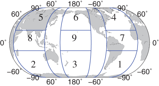
The geographical locations of the 9 separate zones, on which we base our network analysis.
Figure 2. Two examples of typical dynamics of a link strength (W) during the years.
In (a) the distance between the two sites is about 750 Km, the average time delay  (see Section for precise definition) and the variation in the link strength,
  . In (b) the distance between the two sites is about 1500 Km, the average time delay
  and the variation in the link strength, STD(Wl,r) = 0.1.
Figure 3. Distribution of the links variation during time,  in two zones.
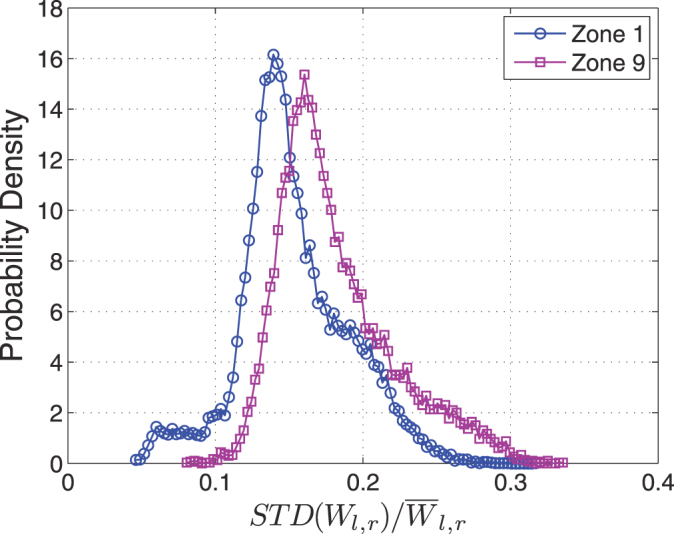
Zone 1 and Zone 9, both for network based on temperature at 850 hPa isobar.
It is known that a typical auto-correlation function for climatological records of a specific node decays as a power law with time4,5,6,7,8,9. Therefore, this stability of the links over many years is surprising and suggest that one might be able to extract new information from the links between the nodes.
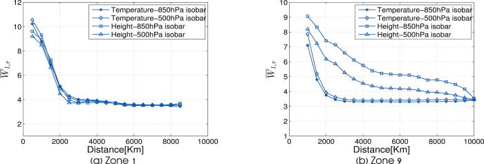
Analyzing the influence of spatial distances D, between the nodes on the strength WD of the link leads to the observation of a strong dependence of WD on D (Fig. 4). Here  is the average over all link strengths W at distance D, and over all years, y. It is seen that for D > 2000 Km, WD reaches a low and almost constant value. This constant value can be regarded (as will be seen in Sec ) as the level of noise. However, we observe a significant difference in this dependence between networks located in equatorial regions and networks located in non-equatorial regions (compare Fig. 2a and Fig. 2b). In networks located in equatorial regions (zones 7-9), WD decreases significantly slower with distance compared to other regions. This difference mainly appears in networks based on the geopotential height field.
Figure 4. The dependence of  on Dl,r in two typical locations.
(a) Zone 1 (off–equatorial region). (b) Zone 9 (equatorial region). The four curves describe four networks which are based on geopotential height measurement at 850 and 500 hPa isobar and based on temperature measurement at 850 and 500 hPa isobar.
Stability of the entire network
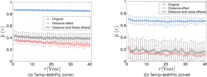
In Sec. we showed that single links remain relatively stable. In this section we study the stability of the entire hierarchy of links within the climate network. We find the network pattern to be relatively stable over time in contrast to the pattern of the daily data itself. This stability of the network may be demonstrated by measuring the similarity between network states in different years. We analyze the similarity by calculating p(τ) (the Pearson coefficient) between the adjacency matrices (representing links) of two network states in different years y1, y2 as a function of τ, where τ = y2 – y1. In this calculation every link in the adjacency matrix representing the year y1 is matched only with the same link in the adjacency matrix representing the year y2. In Fig. 5 (the upper curve) we show the average similarity  between network structures as a function of the time separation τ. It is seen in Fig. 5a that this similarity is indeed high and almost constant,
  . This behavior is consistent for all networks in the non-equatorial regions. For networks in equatorial regions the correlation between the network states in different years,
  is lower than non-equatorial regions, but still significantly high. In addition
  of equatorial regions is more fluctuative. (see Fig. 5b).
Figure 5. The average correlation,  , between network adjacency matrices at different time snapshot, between τ = 1 and τ = 40 years apart, for networks based on temperature at 850 hPa and located at (a) zone 1, and (b) zone 9.
The upper curve in each figure, represents the correlation between the original networks without removing the effects of distance and noise. The standard deviation is calculated from all pairs of years y, y + τ. The lower curve represents  for a network after removing of the distance effect. The mid curve represents
  for a network after removing both, distance and noise effects.
Fig. 4 shows the existence of a strong dependence between the link strength, W and the link distance, D. Links with shorter distances D are therefore more likely to have higher W values, at all times. It is therefore plausible that the high stability of  is partially due to this strong dependence. The contribution of the effect of the W–D dependence to this observed stability, on the one hand, and the contribution of physical coupling processes, on the other hand, should be estimated.
We achieve this goal of removing the contribution of the W–D dependence by subtracting from each link strength, Wl,r the average strength of the group of links with a similar distance,  . A new, transformed adjacency matrix,
  , is thus formed, which does not depend on D. Repeating our analysis of calculating
  , for the new adjacency matrix, we show in the lower curve of Fig. 5, the stability of this network. Indeed, after removal of the distance effect, the network exhibits lower
  values. However, the stability related to physical coupling processes is still significant. Similar analysis with shuffled data yields values which are smaller by typically a factor of 10.
It is plausible that some of our network links emerge mainly due to noise and not due to real physical coupling processes. In Sec. we show that this group of false links is characterized by low Wl,r values at all years, and that this characterization is sufficient for uniquely identifying this group. To identify this group of false links which are due to noise, we define  as the average strength of a link
  over all years. Upon eliminating low weighted links that satisfy
  (where θ is a threshold that will be determined later in Sec. ) from our network, we observe in the middle curve of Fig. 5 an increase of the network stability. Thus, while the hierarchy of false links rapidly changes in each time step, the hierarchy of significant links (having
  ) is, to a large extent, preserved.
The new  values, which are calculated after the removal of both the distance effect and the effects of noise, for different regions and fields are summarized in Table 1. In contrast to the common
  value that was observed for the original network (including the distance and noise effects), after removal of the distance and noise effects we observe lower
  values specific to each zone and climate variable. Still, in general, non equatorial regions exhibit larger stability values than equatorial regions.
Table 1. The average correlation values,  , between network adjacency matrices at different time snapshot for networks based on various fields and located at different regions. The values shown are after removing the distance and noise effects.
| climate variable | Net.Temp | Net.Temp | Net.Height | Net.Height |
| zone | isobar:850 hPa | isobar:500 hPa | isobar:850 hPa | isobar:500 hPa |
| zone 1 | 0.42 ± 0.08 | 0.31 ± 0.08 | 0.48 ± 0.08 | 0.3 ± 0.1 |
| zone 2 | 0.4 ± 0.08 | 0.33 ± 0.08 | 0.32 ± 0.11 | 0.3 ± 0.11 |
| zone 3 | 0.27 ± 0.09 | 0.21 ± 0.1 | 0.17 ± 0.13 | 0.18 ± 0.11 |
| zone 4 | 0.32 ± 0.08 | 0.24 ± 0.09 | 0.45 ± 0.11 | 0.36 ± 0.1 |
| zone 5 | 0.42 ± 0.1 | 0.34 ± 0.1 | 0.51 ± 0.12 | 0.42 ± 0.11 |
| zone 6 | 0.43 ± 0.08 | 0.41 ± 0.09 | 0.45 ± 0.08 | 0.37 ± 0.08 |
| zone 7 | 0.22 ± 0.11 | 0.37 ± 0.15 | 0.37 ± 0.16 | 0.18 ± 0.17 |
| zone 8 | 0.33 ± 0.13 | 0.19 ± 0.14 | 0.24 ± 0.15 | 0.14 ± 0.21 |
| zone 9 | 0.25 ± 0.14 | 0.2 ± 0.11 | 0.37 ± 0.14 | 0.16 ± 0.2 |
It has been shown that during El-Niño times, link strengths,  , are significantly reduced mainly in equatorial regions19,22. Hence our observation of lower stability in equatorial regions is consistent with the known effect of El-Niño on the climate network.
From Table 1 we see that removing both the distance effect and the effects of noise reveals that the networks in zone 3, at the southern ocean, exhibit low stability,  values similar to the equatorial regions. This similarity of the behavior of the network in zone 3 and the behavior of the network in equatorial regions is consistent with the known local oscillations in zone 3 that correlate with ENSO (El-Niño Southern Oscillation - large fluctuation of heat exchange between the ocean and the atmosphere in the Pacific Ocean), due to both ocean mechanisms35 and atmospheric coupling mechanism36.
Based on the high stability values seen in Table 1, we conclude that similarity between network states at all times stems from a hierarchy of real physical correlations (links) between different locations, which is preserved in time.
Similarity between the networks structure, in different altitudes and different climate variables
A further indication that the stability of the network structure reflects a stability of physical coupling processes, is from the finding of similarity between the networks structure in different altitudes, and different climate variables. For example, synchronized heating of two sites at the 850 hPa isobar network is likely to also cause synchronized heating of the corresponding sites in the adjacent isobar of 500 hPa network by direct heat transport. Indeed a recent study of the interaction between climate networks that represent different layers by Donges et.al.(37) suggests that the coupling might be due to convective heat transfer between these layers. In the following we show that such a correspondence between networks of different altitudes and climate variables indeed exists.
In Fig. 6 we show the Pearson correlation py between the adjacency matrices of the climate networks in the 850 hPa isobar and in the 500 hPa as a function of time. Similar to Sec. the upper curve represents the values of py for the original networks, the lower curve is after the removal of the distance effect, and the middle curve is after the removal of both distance and noise effects. As is clearly seen from Fig. 6a this correlation is significant, with an average value of  and small fluctuation during time. In all off–equatorial (for both temperature and geopotential height) regions we observe similar high
  values. A further observation from Fig. 6a is the increase of 10–20% in
  values after the removal of noise.
Figure 6. The correlation between two network adjacency matrices at different altitudes, 850 hPa isobar and 500 hPa isobar in equatorial and off–equatorial regions.
(a) Zone 1 (off–equatorial region), and (b) zone 9 (equatorial region). The upper curve in each figure, represents the correlation between the original networks without removing effects of distance and noise. The lower curve represents py for the networks after removing the distance effect. The mid curve represents py for the networks after removing both, distance and noise effects.
In contrast, in equatorial regions (see e.g. Fig. 6b) we generally observe lower and more fluctuative py values. Another difference between off–equatorial and equatorial regions is the smaller effect of the removal of noise on the py.
Based on physical considerations it is reasonable that a pair of networks with a larger altitude distance will have a smaller similarity. Indeed such a monotonic decreasing relation is seen in Fig. 7. Each point in the curves of Fig. 7 is an average over different regions, different time snapshots, and different altitudes of the correspondence  . The different curves indicate that this monotonic decrease in the similarity behavior holds both in equatorial and off–equatorial regions and both for temperature and geopotential height networks.
Figure 7. Average correlations between pairs of networks with different altitude distances.
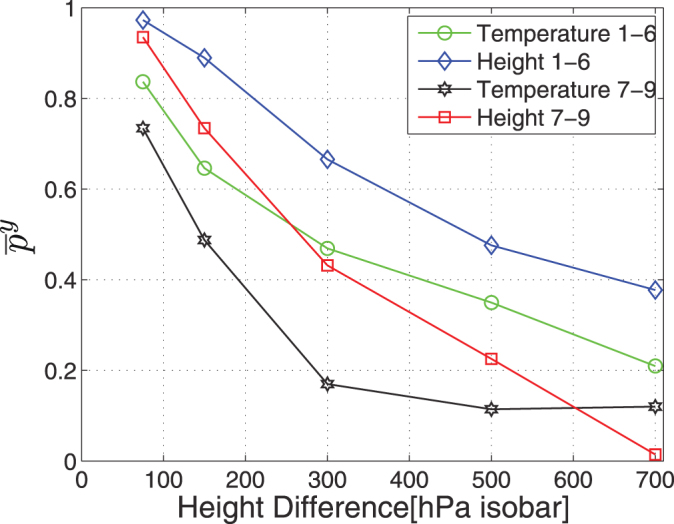
The four curves describe two networks which are located in off–equatorial regions (zones 1–6) and based on geopotential height or based on temperature and two networks which are located in equatorial regions (zones 7–9) and based on geopotential height or based on temperature measurements.
Criterion for significant links
Underlying our supporting arguments for the stability of the climate network, there is an assumption. We rely on the existence of a sharp boundary between the properties of links that result due to noise, LN, and links that result due to real physical dependence, LP. The set of all links is  . In this section we will show that such a boundary indeed exists, with respect to two link properties: (a) the average over all years of the link strength,
  and (b) the variability over time of the time delays of links STD(Tl,r) (STD means standard deviation). We will later show that using both quantities in order to identify the set of physical links LP and the set of noise links LN converge to almost the same sets of links.
Our anchor for comparison between the derived LP and LN is the distributions of (a)
 and (b)
STD(Tl,r) for networks based on shuffled data. The shuffling scheme is aimed at preserving all the statistical quantities of the data, such as the distribution of values, and their autocorrelation properties, but omitting the physical dependence between different nodes (different geographical locations). The network properties in such a case are only due to the statistical quantities and therefore are similar in their properties to false links. To achieve this shuffling goal, we choose for each node a random sequence of y in
  (the order of the days d in each year y is preserved). Thereafter, the entire construction of the network, based on correlations of the shuffled records, is performed. The adjacency matrix of the network based on shuffled data is denoted as wl,r. The time delay matrix of the network based on shuffled data is denoted as tl,r.
(a) Average link strength
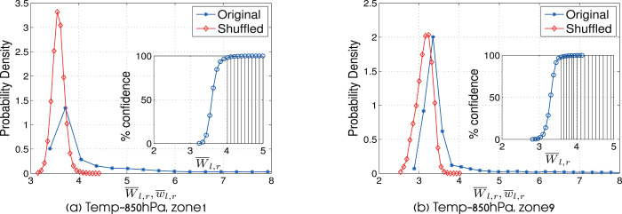
In Fig. 8 we compare the probability density function (PDF) of  and
and  . As clearly seen from these figures, the range of possible
  is extended only over a limited range of values,
  . Higher values that exist in the PDF for
  are missing from the PDF of the shuffled data, and therefore are not likely to occur by chance. The cumulative distribution function (CDF) of
  (see insets of Fig. 8) can be regarded as an estimate for the likelihood of a
  value to arise by real physical dependence. The 98% likelihood level is shaded in the inset of Fig. 8a, having
  for off-equatorial regions, and in the inset of Fig. 8b,
  for equatorial regions.
Figure 8. The distribution of  and
and  in equatorial and off–equatorial regions for networks based on temperature measurements at 850 hPa isobar.
(a) Zone 1 (off–equatorial region), and (b) zone 9 (equatorial region).
(b) Variation of the time delay
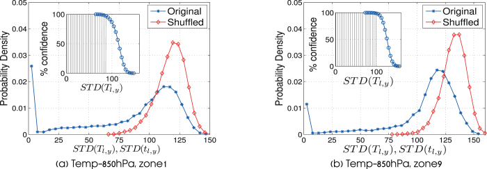
High variability during different years of the time delays of links STD(Tl,r), is also a signature of artificial (random) behavior34. Therefore it serves as another good separator between LP and LN. In Fig. 9 we show the probability density function (PDF) of STD(Tl,r) and STD(tl,r). As clearly seen from these figures, the range of possible STD(tl,r) is extended over a limited range of values, STD(tl,r) ∈ [75, 150]. Lower values that exist in the PDF of STD(Tl,r) are missing from the PDF of the shuffled data, and therefore are not likely to arise by chance. The cumulative distribution function (CDF) of STD(tl,r) (see inset of Fig. 9) can be regarded as an estimate for the likelihood of a STD(Tl,r) value to occur by real physical dependence. The 98% likelihood level is shaded in the inset of Fig. 9, having STD(Tl,r) ≤ 75 for off-equatorial regions, and STD(Tl,r) ≤ 80 for equatorial regions.
Figure 9. The distribution of STD(Tl,r) and STD(tl,r) in equatorial and off–equatorial regions for networks base on temperature measurements at 850 hPa isobar.
(a) Zone 1 (off–equatorial region), and (b) zone 9 (equatorial region).
Both  and STD(Tl,r) can be used for determining a boundary between LP and LN. Convergence to similar LP and LN in both criteria can be considered as a confirmation that either of these criteria indeed efficiently distinct between links that emerge merely due to noise and real links. In Fig. 10 we show a two dimensional PDF of
  and STD(Tl,r). A large fraction of the links evidently have both low values of
  and high values of STD(Tl,r), which is a typical behavior of links that emerge from random behavior. This set of links is realized as a sharp local maximum of the PDF in the region
  , STD(Tl,r ∈ [75, 150] (See Figs. 8 and 9). Within this region,
  and STD(Tl,r) are not correlated, since the fluctuations are random in both axes. Outside this region the mutual local maximum of the PDF in both axis are correlated, i.e. larger values of
  are paired with lower values of STD(Tl,r). The crossover between the two regimes occurs in
  , STD(Tl,r) = 75. This qualitative behavior is consistent at all regions (1–9), but the crossover point is a bit different for off–equatorial regions where
  , STD(Tl,r) = 75.
Figure 10.
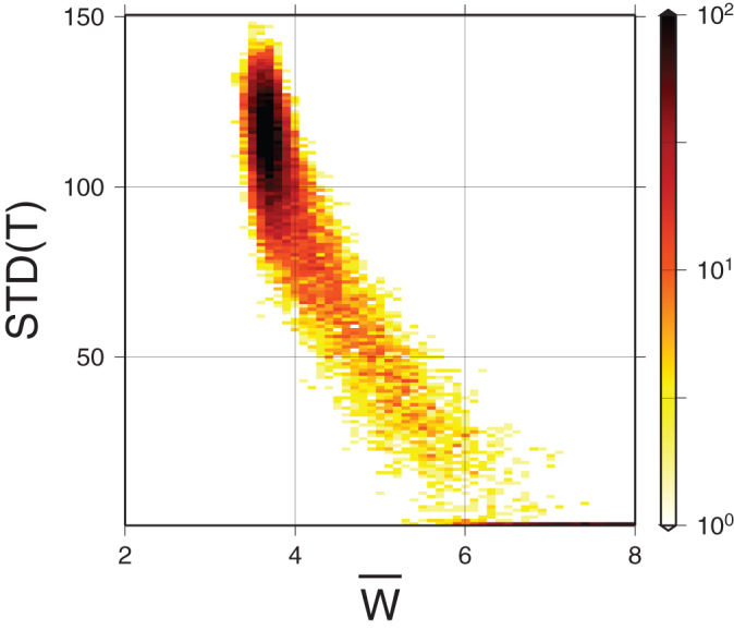
The 2D histogram of links time delay variation, STD(Tl,r) and links average strength,  . This 2D histogram is for network located at zone 1 and based on temperature measurements at 850 hPa isobar.
A further indication that the boundary between LP and LN is within the region  is the increased sensitivity of the stability measure
  to the removal of noise within this region. Here we indicate explicitly the value of the threshold for noise removal by the second argument θ. In Fig. 11 we show the differential of
  , averaged over all values of τ,
  , where δθ = 0.5. We find a sharp local maximum in δp, around
  . This sharp maximum is consistent with θ crossing the boundary between LN and LP, where many of the links related to noise drop off the network, and causes the average stability
  to abruptly rise. Such behavior of δp is consistent both in equatorial regions (stars) and off–equatorial regions (circles). The response of the sensitivity δp to further removal of links (which mainly belong to LP) is thereafter reduced. In fact, removal of real physical links might even result in a reduction of the stability (e.g. δp < 0), as is indeed observed for large θ in the equatorial curve in Fig. 11. In conclusion, a sharp boundary between LN and LP is almost certainly identified around
  in the networks calculated for all types of data (temperature and geopotential height in various altitudes covering the troposphere), both in equatorial and off–equatorial regions.
Figure 11.
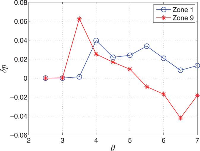
The sensitivity, δp, of the stability function p as a function of the threshold θ.
Discussion
We have established the stability of the network of connections between the dynamics of climate variables (e.g. temperatures and geopotential heights) in different geographical regions. This stability stands in fierce contrast to the observed instability of the original climatological field pattern. Thus the coupling between different regions is, to a large extent, constant and predictable. The links in the climate network seem to encapsulate information that is missed in analysis of the original field.
The strength of the physical connection, Wl,r, that each link in this network represents, changes only between 5% to 30% over time. A clear boundary between links that represent real physical dependence and links that emerge due to noise is shown to exist. The distinction is based on both the high link average strength  and on the low variability of time delays STD(Tl,r).
Recent studies indicate that the strength of the links in the climate network changes during the ENSO19,21,22 and the NAO23 cycles. These changes are within the standard deviation of the strength of the links found here. Indeed in Fig. 3 it is clearly seen that the coefficient of variation of links in the El-Niño basin (zone 9) is larger than other regions such as zone 1. Note that even in the El-Niño basin the coefficient of variation is relatively small (less than 30%).
Beside the stability of single links, also the hierarchy of the link strengths in the climate network is preserved to a large extent. We have shown that this hierarchy is partially due to the two dimensional space in which the network is embedded, and partially due to pure physical coupling processes. Moreover the contribution of each of these effects, and the level of noise was explicitly estimated. The spatial effect is typically around 50% of the observed stability, and the noise reduces the stability value by typically 5%–10%.
The network structure was further shown to be consistent across different altitudes, and a monotonic relation between the altitude distance and the correspondence between the network structures is shown to exist. This yields another indication that the observed network structure represents effects of physical coupling.
The stability of the network and the contributions of different effects were summarized in specific relation to different geographical areas, and a clear distinction between equatorial and off–equatorial areas was observed. Generally, the network structure of equatorial regions is less stable and more fluctuative.
The stability and consistence of the network structure during time and across different altitudes stands in contrast to the known unstable variability of the daily anomalies of climate variables. This contrast indicates an analogy between the behavior of nodes in the climate network and the behavior of coupled chaotic oscillators38. While the fluctuations of each coupled oscillators are highly erratic and unpredictable, the interactions between the oscillators is stable and can be predicted. The possible outreach of such an analogy lies in the search for known behavior patterns of coupled chaotic oscillators in the climate system. For example, existence of phase slips in coupled chaotic oscillators is one of the fingerprints for their cooperated behavior39, which is evident in each of the individual oscillators. Some abrupt changes in climate variables, for example, might be related to phase slips, and can be understood better in this context.
On the basis of our measured coefficient of variation of single links (around 15%), and the significant overall network stability of 20–40%, one may speculatively assess the extent of climate change. However, for this assessment our current available data is too short and does not include enough time from periods before the temperature trends. An assessment of the relation between the network stability and climate change might be possible mainly through launching of global climate model “experiments” realizing other climate conditions, which we indeed intend to perform.
A further future outreach of our work can be a mapping between network features (such as network motifs) and known physical processes. Such a mapping was previously shown to exist22 between an autonomous cluster in the climate network and El-Niño. Further structures without such a climate interpretation might point towards physical coupling processes which were not observed earlier.
Methods
Data
We analyze data obtained from a reanalysis project40. The records consist of the reanalysis air temperature field and the geopotential height field h ( , where R is the Boltzmann gas constant for air, T is the temperature, g is the gravitation acceleration, p is the pressure at the current isobar and ps is the refference pressure in the surface level), for the 1000 hPa, 925 hPa, 850 hPa, 700 hPa, 500 hPa and 300 hPa isobars. We use daily values between the years 1948-2006. The data is arranged on a world-wide grid with a resolution of 5° × 5°. We divide the globe into 9 zones (see Fig. 1), in order to identify different network dynamics specific to different zones.
The network construction method
We analyze daily climatological records (temperature/geopotential heights) taken from a grid in various geographical zones (Fig. 1). To avoid the trivial effect of seasonal trends we subtract from the records of each day the yearly average value of that day. Specifically, we take the climatological signal (temperature/geopotential heights) of a given site in the grid to be  , where y is the year and d is the day (ranging from 1 to 365) of that year. The new signal will be
  , where N is the number of years available in the record. For each pair of sites l and r in a specific zone, we compute the absolute value of the cross-covariance function,
  , of their local climatological signals such as temperature/geopotential heights in the range of time delays τ ∈ [−τmax, τmax] integrated over a specific year (y) (see Fig. 12). To quantify the significance of the correlation between nodes l and r we normalize the nominal value of the maximal observed correlation by its standard deviation. We therefore define the strength of the link to be
  , where < … >, MAX and STD are the mean value, maximal value and the standard deviation of
  in the range of τ, respectively. The matrix
  represents the weighted adjacency matrix of the network at year y. The time shift at which
  is maximal is defined as the link time delay, and denoted as
  .
.
Figure 12. A typical cross-covariance function between two sites, representing the level of correlation within a time lag ranging from −τmax to +τmax where τmax = 220.
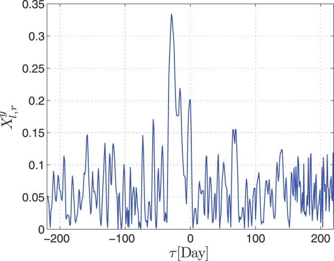
In the current example  ,
,  .
.
Author Contributions
B.Y., G.A., G.O. and H.S. performed the calculations, analyzed the results and wrote the paper.
Acknowledgments
We thank the LINC and the Epiwork EU projects, the DFG, and the Israel Science Foundation for support.
References
- Lorenz E. N. Deterministic nonperiodic flow. J. Atmos. Sci. 20, 130141 (1963). [Google Scholar]
- Collins M. Climate predictability on interannual to decadal time scales: the initial value problem. Climate Dynamics 19, 671–692 (2002). [Google Scholar]
- Madden R. A. Estimates of the natural variability of time-averaged sea-level pressure. J. Atmos. Sci. 104, 942 (1976). [Google Scholar]
- Koscielny-Bunde E. et al. Indication of a universal persistence law governing atmospheric variability. Phys. Rev. Lett. 81, 729 (1998). [Google Scholar]
- Bunde E. K., Roman H. E., Bunde A., Havlin S. & Schellnhuber H. J. Long-range power-law correlations in local daily temperature fluctuations. Philosophical Magazine Part B 77, 1331–1340 (1998). [Google Scholar]
- Pelletier J. & Turcotte D. Self-affine time series: II. applications and models. Advances in Geophysics 40, 91–166 (1999). [Google Scholar]
- Eichner J. F., Koscielny-Bunde E., Bunde A., Havlin S. & Schellnhuber H.-J. Power-law persistence and trends in the atmosphere: A detailed study of long temperature records. Phys. Rev. E 68, 046133 (2003). [DOI] [PubMed] [Google Scholar]
- Bunde A., Eichner J. F., Kantelhardt J. W. & Havlin S. Long-term memory: A natural mechanism for the clustering of extreme events and anomalous residual times in climate records. Phys. Rev. Lett. 94, 048701 (2005). [DOI] [PubMed] [Google Scholar]
- Santhanam M. & Kantz H. Long-range correlations and rare events in boundary layer wind fields. Physica A: Statistical Mechanics and its Applications 345, 713–721 (2005). [Google Scholar]
- Chen D., Cane M. A., Kaplan A., Zebiak S. E. & Huang D. Predictability of El-Niño over the past 148 years. Nature 428, 733–736 (2004). [DOI] [PubMed] [Google Scholar]
- Tsonis A. A., Swanson K. L. & Roebber P. J. What do networks have to do with climate? Bull. Am. Meteorol. Soc. 87, 585–595 (2006). [Google Scholar]
- Albert R. & Barabási A.-L. Statistical mechanics of complex networks. Rev. Mod. Phys. 74, 47–97 (2002). [Google Scholar]
- Boccaletti S., Latora V., Moreno Y., Chavez M. & Hwang D. Complex networks: Structure and dynamics. Physics Reports 424, 175–308 (2006). [Google Scholar]
- Arenas A., Díaz-Guilera A., Kurths J., Moreno Y. & Zhou C. Synchronization in complex networks. Physics Reports 469, 93–153 (2008). [Google Scholar]
- Earl M. G. & Strogatz S. H. Synchronization in oscillator networks with delayed coupling: A stability criterion. Phys. Rev. E 67, 036204 (2003). [DOI] [PubMed] [Google Scholar]
- Bonanno G., Caldarelli G., Lillo F. & Mantegna R. N. Topology of correlation-based minimal spanning trees in real and model markets. Phys. Rev. Lett. 68, 046130 (2003). [DOI] [PubMed] [Google Scholar]
- Donges J. F., Zou Y., Marwan N. & Kurths J. The backbone of the climate network. Europhys. Lett. 87, 48007 (2009). [Google Scholar]
- Donges J. F., Zou Y., Marwan N. & Kurths J. Complex networks in climate dynamics - comparing linear and nonlinear network construction methods. Eur. Phys. J. Special Topics 174, 157–179 (2009). [Google Scholar]
- Yamasaki K., Gozolchiani A. & Havlin S. Climate networks around the globe are significantly affected by El Niño. Phys. Rev. Lett. 100, 228501 (2008). [DOI] [PubMed] [Google Scholar]
- Gozolchiani A., Yamasaki K., Gazit O. & Havlin S. Pattern of climate network blinking links follows El Niño events. Europhys. Lett. 83, 28005 (2008). [Google Scholar]
- Tsonis A. A. & Swanson K. L. Topology and predictability of El Niño and La Niña networks. Phys. Rev. Lett. 100, 228502 (2008). [DOI] [PubMed] [Google Scholar]
- Gozolchiani A., Havlin S. & Yamasaki K. The Emergence of El-Niño as an Autonomous Component in the Climate Network. Phys. Rev. Lett. 107, 148501 (2011). [DOI] [PubMed] [Google Scholar]
- Guez O., Gozolchiani A., Berezin Y., Brenner S. & Havlin S. Climate network structure evolves with north atlantic oscillation phases. EPL (Europhysics Letters) 98, 38006 (2012). [Google Scholar]
- Watts D. J. & Strogatz S. H. Collective dynamics of ‘small-world’ networks. Nature 393, 440 (1998). [DOI] [PubMed] [Google Scholar]
- Newman M. E. J. The structure and function of complex networks. SIAM Review 45, 167–256 (2003). [Google Scholar]
- Cohen R. & Havlin S. Complex Networks: Structure, Robustness and Function (Cambridge University Press, 2010). [Google Scholar]
- Dunne J. A., Williams R. J. & Martinez N. D. Network structure and biodiversity loss in food webs: robustness increases with connectance. Ecology Letters 5, 558–567 (2002). [Google Scholar]
- Jeong H., Mason S. P., Barabasi A. L. & Oltvai Z. N. Lethality and centrality in protein networks. Nature 411, 41–42 (2001). [DOI] [PubMed] [Google Scholar]
- Carmi S., Levanon E. Y., Havlin S. & Eisenberg E. Connectivity and expression in protein networks: Proteins in a complex are uniformly expressed. Phys. Rev. E 73, 031909 (2006). [DOI] [PubMed] [Google Scholar]
- Bouchaud J.-P. & Mzard M. Wealth condensation in a simple model of economy. Physica A: Statistical Mechanics and its Applications 282, 536–545 (2000). [Google Scholar]
- Dorogovtsev S. N. & Mendes J. F. F. Evolution of Networks: From Biological Nets to the Internet and WWW (Oxford University Press, 2003). [Google Scholar]
- Barrat A., Barthelemy M., Pastor-Satorras R. & Vespignani A. The architecture of complex weighted networks. PNAS 101, 3747–3752 (2004). [DOI] [PMC free article] [PubMed] [Google Scholar]
- Caldarelli G. & Vespignani A. Large scale structure and dynamics of complex networks: from information technology to finance and natural science (World Scientific, 2007). [Google Scholar]
- Bashan A., Bartsch R. P., Kantelhardt J. W., Havlin S. & Ivanov P. C. Network physiology reveals relations between network topology and physiological function. Nature Communications 3, 702 (2012). [DOI] [PMC free article] [PubMed] [Google Scholar]
- White W. B. & Peterson R. G. An Antarctic circumpolar wave in surface pressure, wind, temperature and sea-ice extent. Nature 380, 699–702 (1996). [Google Scholar]
- Liu J., Yuan X., Rind D. & Martinson D. G. Mechanism study of the ENSO and southern high latitude climate teleconnections. Geophys. Res. Lett 14, 1679 (2002). [Google Scholar]
- Donges J. F., Schultz H. C. H., Marwan N., Zou Y. & Kurths J. Investigating the topology of interacting networks - theory and application to coupled climate subnetworks. Eur. Phys. J. B 84, 635 (2011). [Google Scholar]
- Boccaletti S., Kurths J., Osipov G., Valladares D. L. & Zhou C. S. The synchronization of chaotic systems. Phys. Rep. 366, 1 (2002). [Google Scholar]
- Zheng Z., Hu G. & Hu B. Phase slips and phase synchronization of coupled oscillators. Phys. Rev. Lett. 81, 5318 (1998). [Google Scholar]
- Kanamitsu M. et al. NCEPDOE AMIP-II Reanalysis. (R-2) (2002).


