3.5D dynamic PET image reconstruction incorporating kinetics-based clusters

Abstract

Standard 3D dynamic PET imaging consists of independent image reconstructions of individual frames followed by application of appropriate kinetic model to the time activity curves (TACs) at the voxel or region-of-interest. The emerging field of 4D PET reconstruction, by contrast, seeks to move beyond this scheme and incorporate information from multiple frames within the image reconstruction task. Here we propose a novel reconstruction framework aiming to enhance quantitative accuracy of parametric images via introduction of priors based on voxel kinetics, as generated via clustering of preliminary reconstructed dynamic images to define clustered neighborhoods of voxels with similar kinetics. This is then followed by straightforward maximum a posterior (MAP) 3D PET reconstruction as applied to individual frames; and as such the method is labeled “3.5D” image reconstruction. The use of cluster-based priors has the advantage of further enhancing quantitative performance in dynamic PET imaging, because: (a) there are typically more voxels in clusters than in conventional local neighborhoods, and (b) neighboring voxels with distinct kinetics are less likely to be clustered together. Using realistic simulated ¹¹C-raclopride dynamic PET data, the quantitative performance of the proposed method was investigated. Parametric distribution-volume (DV) and DV ratio (DVR) images were estimated from dynamic image reconstructions using (a) MLEM, and MAP reconstructions using (b) the quadratic prior (QP-MAP), (c) the Green prior (GP-MAP) and (d, e) two proposed cluster-based priors (CP-U-MAP and CP-W-MAP), followed by graphical modeling, and were qualitatively and quantitatively compared for 11 regions-of-interest (ROIs). Overall, the proposed dynamic PET reconstruction methodology resulted in substantial visual as well as quantitative accuracy improvements (in terms of noise vs. bias performance) for parametric DV and DVR images. The method was also tested on a 90 min ¹¹C-raclopride patient study performed on the high-resolution research tomography. The proposed method was shown to outperform the conventional method in visual as well as quantitative accuracy improvements (in terms of noise vs. regional DVR value performance).

1. Introduction

Positron emission tomography (PET) is a powerful molecular imaging modality enabling measurements of radiotracer distributions in vivo. Typically, dynamic scans are performed to measure quantitative changes over time in the bio-distribution of radiopharmaceuticals throughout a target structure or the organs of interest. Physiological and/or biochemical parameters are then derived with the additional use of tracer kinetic modeling techniques (Bentourkia and Zaidi, 2007). These parameters are often crucial for interpreting dynamic PET data and to better differentiate between normal and diseased tissues.

Traditionally, standard 3D dynamic PET imaging consists of independent image reconstructions at individual frames followed by application of appropriate kinetic model to the time activity curves (TACs) at the voxel or ROI level (Rahmim and Zaidi, 2008). However, conventional 3D dynamic PET image reconstruction is challenged by the limited statistical quality of the 3D images obtained from individual data frames, especially within the context of continuing demands for improved spatiotemporal resolution. Independent-frame 3D image reconstruction is commonly accomplished using statistical image reconstruction methods (Leahy and Qi, 2000), such as maximum likelihood (ML) or maximum a posterior (MAP) expectation-maximization (EM) methods. Direct ML estimates of PET images exhibit high variances at low counts (Reader and Zaidi, 2007). This problem of low counts is further accentuated with increased temporal sampling (i.e. use of increased number of dynamic frames in a certain time period).

Bayesian methods attempt to tackle this ill-posedness inherent in PET image reconstructions through the introduction of prior models (Leahy and Qi, 2000). Conventional priors focus on local neighborhoods and subsequently penalize inter-voxel intensity differences through different penalty functions such as the quadratic prior (Geman and Geman, 1984). Nevertheless, a drawback of these conventional priors is that they only consider pre-defined local neighborhoods to define the prior at any given position. Furthermore, they may lead to blurring of edges. To this end, a number of more sophisticated priors have been proposed to allow enhanced tolerance for edges including the median prior (Hsiao et al., 2003) and priors whose gradients level off with increasing differences such as the Geman (Geman et al., 1987), Huber (Mumcuoglu et al., 1996), Green (Green, 1990) and Nuyts (Nuyts et al., 2002) priors.

An alternative approach seeks to control penalization of inter-voxel differences across edges via incorporation of information obtained from anatomical images (e.g. Lipinski et al., 1997; Comtat et al., 2002; Baete et al., 2004). More sophisticated anato-functional priors have also appeared in the literature (e.g. Rangarajan et al., 2000; Somayajula et al., 2011; Vunckx et al., 2011; Tang and Rahmim, 2009). Ultimately, however, while many types of PET imaging tasks exhibit correlations between anatomy and radio-pharmaceutical uptake, the relationship can be complex and indirect. The proposed framework seeks an approach in which ‘functional neighborhoods’ of similar kinetics are identified via clustering methods, and are incorporated as priors within the reconstruction task.

In the different context of post-reconstruction dynamic PET image analysis, a number of clustering-based techniques were previously proposed to either better facilitate segmentation or to reduce noise in kinetic analysis (by grouping and concurrent analysis of voxels with similar kinetics). In segmentation, this included the use of K-means-like clustering applied to segment dynamic brain images (Wong et al., 2002; Liptrot et al., 2004). Fuzzy C-mean (FCM) clustering, also known as soft K-mean clustering, as well as mixture models making multivariate Gaussian or non-Gaussian assumptions (using EM or ICA methods) were also proposed to segment dynamic brain images (Koivistoinen et al., 2004). In dynamic cardiac PET imaging, factor analysis was applied to segment and estimate left and right ventricular input functions automatically (El Fakhri et al., 2005). In oncologic whole-body imaging, the PCA approach was used by Anzari et al. (1999) to enhance distinction of tumors in dynamic FDG images compared to conventional static standard uptake value (SUV) images. Janssen et al. (2009) instead used K-means clustering applied to slopes of TACs (calculated based on last few time frames of FDG uptake) to differentiate between tumors and healthy tissues.

In the context of kinetic analysis, clustering analysis for kinetics (CAKS) by Kimura et al. was originally based on a single-compartment model (Kimura et al., 1999) but was also extended to the irreversible two-compartment FDG model (k₄ assumed 0) using principle component analysis (PCA) (Kimura et al., 2002) and also supplemented by a mixed Gaussian model to better facilitate PCA classification in the presence of noise (Kimura et al., 2001). Two other approaches applied and evaluated in brain research PET include hierarchical cluster analysis with average linkage method (Zhou et al., 2002); or combined hierarchical and K-means cluster analysis (Huang et al., 2007).

In contrast to abovementioned post-reconstruction methods, the present work utilizes clustering to enhance the image reconstruction task itself, via generation of kinetics-based clusters of neighborhoods. The approach is labeled “3.5D” image reconstruction, because on the one hand it is related to the emerging field of spatiotemporal 4D PET reconstruction (Rahmim et al., 2009) which attempts to move beyond independent-frame reconstructions (see also discussion in Sec. 5.3) while on the other hand, the final reconstruction step includes straightforward application of maximum a posteriori (MAP) reconstruction to the original individual dynamic frames without the need for advanced transforms, temporal basis functions, or kinetic models as pursued in the 4D reconstruction framework.

2. Methods

2.1. MAP image reconstruction

Let f_m ∈ R^n_j denote the emission distribution in time frame m (1 ≤ m ≤ M). The PET data, modeled as a collection of independent Poisson random variables with expectation g̅_m ∈ R^n_i in time frame m, can be related to f_m through an affine transform:

$${\mathbf{g̅}}_m(\mathbf{f})={\mathbf{\text{Af}}}_m+{\mathbf{r}}_m,$$ (1)

where A ∈ R^n_i×n_j is the system matrix with element (i, j) denoting the probability of a positron emitted from voxel j resulting in a coincidence at the ith detector pairs, and r_m ∈ R^n_i accounts for the scattered and random events in frame m, and n_i and n_j denote the total number of detector pairs and voxels, respectively.

According to the measurement model, the log-likelihood function of the dynamic data set is given by

$$L(\mathbf{g}|\mathbf{f})={\displaystyle \sum _{m=1}^M}{\displaystyle \sum _{i=1}^{n_i}}{g}_{\mathit{\text{im}}}\text{ log }{\mathrm{g̅}}_{\mathit{\text{im}}}(\mathbf{f})-{\mathrm{g̅}}_{\mathit{\text{im}}}(\mathbf{f}),$$ (2)

where g={g_m} and f={f_m} denote the measured dynamic sinograms and the unknown emission distributions, respectively.

Maximum likelihood (ML) estimation attempts to maximize L(g | f) with respect to f. However, ML estimation will produce increasing noise levels with increasing iterations. A powerful method to circumvent daunting noise levels is to utilize Bayesian theory to maximize the posterior probability that includes prior image information. The prior information can be specified by a probability density on f and subsequently combined with the information contained in g to produce an estimation of the unknown image. Commonly, the prior is modeled to follow a Gibbs distribution

$$P(\mathbf{f})\propto \text{exp}\{-\beta U(\mathbf{f})\},$$ (3)

where U(f) is the energy function and β is a regularization parameter that controls the tradeoff between resolution and noise. Combining the likelihood function and the image prior, MAP estimation of f is given by

$$\mathbf{f̂}=\mathit{\text{arg }}\underset{\mathbf{f}\ge \mathbf{0}}{\mathit{\text{max}}}\{L(\mathbf{g}|\mathbf{f})-\beta U(\mathbf{f})\}.$$ (4)

Based on equations (2) and (4), we then invoke the one-step-late (OSL) approach for an iterative update to the MAP estimate (Green, 1990):

$$f_{\mathit{\text{jm}}}^{\mathit{\text{new}}}=\frac{f_{\mathit{\text{jm}}}^{\mathit{\text{old}}}}{{\displaystyle {\sum }_i}{a}_{\mathit{\text{ij}}}+\beta \frac{\partial U(\mathbf{f})}{\partial f_{\mathit{\text{jm}}}}{|}_{f_{\mathit{\text{jm}}}=f_{\mathit{\text{jm}}}^{\mathit{\text{old}}}}}{\displaystyle \sum _i}\frac{a_{\mathit{\text{ij}}}{g}_{\mathit{\text{im}}}}{{\displaystyle {\sum }_j}{a}_{\mathit{\text{ij}}}{f}_{\mathit{\text{jm}}}^{\mathit{\text{old}}}+r_{\mathit{\text{im}}}},$$ (5)

where the new estimate of voxel j in time frame m is updated from the old estimate. A single bin i in mth frame of the measured dynamic sinograms g is represented by g_im, and a_ij represents an element of the system matrix A. The performance of the MAP reconstruction strongly depends on the construction of the prior U(f) and the regularization parameter β, and then we will elaborate them in section 2.2 and 2.3, respectively.

2.2. Generation of the prior model

2.2.1. Conventional localized priors

The prior energy function U (f) in (5) is commonly computed via a weighted sum of potential functions v of the differences between voxels in the local neighborhood N_j:

$$U(\mathbf{f})={\displaystyle \sum _{m=1}^M}{\displaystyle \sum _{j=1}^{n_j}}{\displaystyle \sum _{k\in N_j}}{w}_{\mathit{\text{kj}}}v(f_{\mathit{\text{km}}}-f_{\mathit{\text{jm}}}),$$ (6)

where w_kj is the weight of a given pixel k in the neighborhood of pixel j. For 3D reconstructions, a neighborhood with 18 neighbors was selected. The weight w_kj is set to 1 if k and j are orthogonal nearest neighbors, to $\sqrt{1/2}$ for diagonal neighbors and to 0 otherwise. Generally, different choices of potential function v lead to different priors. The prior becomes quadratic prior (QP) when the potential function v takes the form of v(u) = u². We also considered Green’s prior (GP) where the potential function v is set to v(u) = log cosh(u/δ), where δ is a free parameter to be optimized (Green 1990).

2.2.2. The proposed cluster-based prior

In order to make use of more voxels to further encourage smoothing without causing significant bias, we expanded the use of localized neighborhoods to those containing all voxels with similar temporal behaviors as clustered together. We continue to use the quadratic potential function, nonetheless the neighborhood definitions are now different:

$$U^{*}(\mathbf{f})={\displaystyle \sum _{m=1}^M}{\displaystyle \sum _{j=1}^{n_j}}{\displaystyle \sum _{k\in c\{j\}}}{w}_{\mathit{\text{kj}}}{(f_{\mathit{\text{km}}}-f_{\mathit{\text{jm}}})}^2,$$ (7)

where c{j} stands for the functional cluster in which voxel j is grouped. As for the weight definition, a straight-forward approach is to equally weight all voxels within each neighborhood:

$$w_{\mathit{\text{kj}}}=1/(N_{c\{j\}}-1),$$ (8)

where N_c{j} is the number of voxels in functional cluster c{j}, resulting in what we refer to as the un-weighted cluster-based prior (CP-U).

However, due to noise and/or usage of insufficient number of clusters, some voxel may be incorrectly clustered together, and lead to bias in the MAP reconstructed images. Subsequently, a methodology was developed to alleviate such a bias: namely, distance weighting was introduced to reduce the resulting adverse impact:

$$w_{\mathit{\text{kj}}}=1/d_{\mathit{\text{kj}}},$$ (9)

where d_kj is the Euclidean distance between voxel j and voxel k, resulting in a distance-weighted cluster-based prior (CP-W). In this latter scenario, we only compute w_jk in a particular neighborhood (5×5×5) that is not necessarily as large as the entire cluster, as the weights of more distant voxels within the cluster will be negligible and this can lead to considerable computational speed-up. In turn, this can lead to considerable computational speed up. It is important to note that, relative to most previous applications of MAP reconstruction to emission computed tomography, our proposed cluster-based priors attempt to use neighborhoods that are optimally defined to contain kinetically homogeneous voxels. This can effectively reduce noise levels without causing significant increases in bias for a given temporal sampling scheme.

2.2.3. Clustering of time activity curves (TACs)

The construction of the two priors in Eqs. (7–9) strongly depends on the functional clusters c{j}, which determines how accurately the priors describe the nature of the images. In dynamic PET studies, the temporal behavior of each voxel j can be described by a TAC vector collecting the reconstructed activity estimates of the voxel over time. Instead of separately clustering an individual image based on voxel intensities, as we preliminarily investigated in Lu et al. (2011), here we propose to perform clustering based on voxel dynamic (i.e. TACs). Our aim is to classify the image voxels according to their corresponding TAC shapes and magnitudes so that voxel TACs within a cluster are relatively homogeneous, while voxel TACs drawn from different clusters are relatively heterogeneous. Suppose that there exist K characteristic curves in the dynamic PET image f, the fuzzy C-means clustering approach minimizes

$$J={\displaystyle \sum _{j=1}^{n_j}}{\displaystyle \sum _{k=1}^K}{u}_{\mathit{\text{kj}}}^q{\Vert {\mathbf{f}}_{\mathbf{j}}-{\mathbf{v}}_{\mathbf{k}}\Vert }_{\mathbf{w}}^2,$$ (10)

where ‖.‖ stands for the Euclidian norm, f_j ∈ R^M is the TAC for the jth voxel, v_k ∈ R^M is the centroid TAC of the kth cluster,u_kj is the degree of membership of f_j in the kth cluster, q is the fuzzification parameter, and W ∈ R^M×M is a square matrix containing the weighting factors on the diagonal entries and zeros otherwise. The weighting factors are set as inversely proportional to variances in each dynamic frame m: the estimated variance of OSEM reconstructed images is elaborated in section 2.3.

2.3. Regularization parameter model

The regularization parameter (β in (5)) determines how much a role the prior plays in the reconstruction process. Commonly in the literature, β is equally set amongst different frames, even though different frames demonstrate distinct statistics. Alternatively, we propose the following frame-dependent regularization parameter:

$${\beta }_m=\alpha {\sigma }_m^2,$$ (11)

where α is a scaling factor, and ${\sigma }_m^2$ is the estimated variance for frame m. In fact, this can be seen as an effort to obtain relative consistency in image resolution and noise amongst different frames, given dependence of both image resolution and noise on frame statistics (Qi and Leahy, 2000). Based on the variance model in Yaqub et al. (2006), the variance of a decay-corrected frame is

$${\sigma }_m^2={\text{dcf}}_m\times {\text{dcf}}_m\times {\mathrm{N}}_m/(\mathrm{\Delta }{\mathrm{T}}_m\times \mathrm{\Delta }{\mathrm{T}}_m),$$ (12)

where N_m denotes decay-corrected sinogram counts, ΔT_m represents the frame length, and dcf_m is the decay correction factor. The decay correction factor (for each frame) is given by dcf=λ×(T_e − T_s)/{exp(−λ×T_s)−exp(−λ×T_e)}, where λ is the decay constant;T_s and T_e are the frame start and end times, respectively. A similar frame-varying regularization approach was also applied in (Wang and Qi, 2009a), though the effect of decay correction was not considered or not discussed. For quantitative comparison purposes, we also consider the conventional frame-independent regularization approach as:

$${\beta }_0=\alpha {\sigma }_0^2.$$ (13)

where α is defined as that in (11), and σ₀ is a mean overall statistics measure obtained by averaging σ_m across the frames.

2. 4. The implementation of proposed 3.5D dynamic PET reconstruction

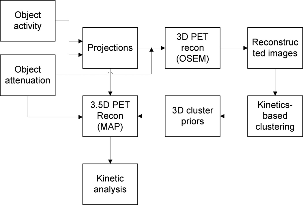
The proposed 3.5D PET reconstruction algorithm is depicted in figure 1. There are three steps elaborated as follows:

• Step 1: The standard 3D MLEM reconstruction (including 3 iterations and 16 subsets) is run to generate a sequence of pre-reconstructed dynamic PET frames ${\mathbf{f}}^{(\mathbf{\text{MLEM}})}=\{{\mathbf{f}}_j^{(\mathbf{\text{MLEM}})}\}$.

• Step 2: The kinetics-based clustering is performed on the pre-reconstructed dynamic frames f^(MLEM). In this case, the dynamic PET images are set to f=f^(MLEM) and the weighting matrix is set to $\mathbf{W}=\mathbf{\text{diag}}\{{\sigma }_1^{-2}\mathbf{,}{\sigma }_2^{-2}\mathbf{,}{\sigma }_M^{-2}\}$. To speed up the computation, we have set the fuzzification parameter q in Eq. (10) as 2, as commonly pursued in the literature (e.g. Ahmed et al., 2002; Chen and Zhang, 2004). The solution (Bezdek, 1981) of the objective function J in Eq. (10) can be obtained through an iterative process, which is carried as follows:

  1. Set the total cluster number K and stopping condition ε.
  2. Randomly initialize the fuzzy partition matrix U⁽⁰⁾ consisting of individual $u_{\mathit{\text{kj}}}^{(0)}$ values.
  3. Set the loop counter b = 0.
  4. Calculate the cluster centers ${\mathbf{v}}_{\mathbf{k}}^{\mathbf{(}\mathbf{b}\mathbf{)}}$ from U^(b)

     $${\mathbf{v}}_{\mathbf{k}}^{\mathbf{(}\mathbf{b}\mathbf{)}}=\frac{{\displaystyle \sum _j}{(u_{\mathit{\text{kj}}}^{(b)})}^q{\mathbf{f}}_j}{{\displaystyle \sum _j}{(u_{\mathit{\text{kj}}}^{(b)})}^q},$$ (14)
  5. Calculate the membership matrix U^(b+1)

     $$u_{\mathit{\text{kj}}}^{(b+1)}=\frac{1}{{\displaystyle \sum _{i=1}^K}{\left(\frac{{\Vert {\mathbf{f}}_{\mathbf{j}}-{\mathbf{v}}_{\mathbf{k}}\Vert }_w^2}{{\Vert {\mathbf{f}}_{\mathbf{j}}-{\mathbf{v}}_{\mathbf{i}}\Vert }_w^2}\right)}^{1/(q-1)}},$$ (15)
  6. If max{U^(b) − U^(b+1)} <ε then stop; otherwise, set b = b + 1 and go to step 4.

• Step 3: 3.5D PET reconstruction (MAP using kinetics-based cluster priors) is followed by kinetic modeling. After the fuzzy partition matrix U is obtained, we determinate the functional cluster c{j} for each voxel j by setting the largest membership value u_kj to 1 and others to 0. Thus, the MAP OSL algorithm (5) is invoked utilizing the proposed cluster-based prior (7) along with the frame-dependent regularization parameter (11).

Figure 1.

The flowchart of the proposed 3.5D dynamic PET reconstruction algorithm.

3. Experimental design

3.1. Simulation study

A two-compartment model (including non-displaceable and bound compartments) (Innis et al., 2007) was used to simulate dynamic PET studies with reversible binding. For a given plasma input C^p(t), the factional plasma volume in tissue V^p, and the four standard rate parameters K₁ (ml/min/g), k₂ (1/min), k₃ (1/min) and k₄ (1/min), the measured total radioactivity C(t) is given by (Bentourkia and Zaidi, 2007):

$$C(t)=\frac{K_1}{{\alpha }_2-{\alpha }_1}[(k_3+k_4-{\alpha }_1)e^{-{\alpha }_{1}t}+({\alpha }_2-k_3-k_4)e^{-{\alpha }_{2}t}]*C^p(t)+V^p{C}^p(t)$$ (16)

where * denotes the convolution operation, and

$$\raisebox{1ex}{${\alpha }_{1,2}=[k_2+k_3+k_4\mp \sqrt{{(k_2+k_3+k_4)}^2-4k_2{k}_4}]$}\!\left/ \!\raisebox{-1ex}{$2$}\right.$$ (17)

For our simulations, we used 55 ¹¹C-raclopride dynamic PET human scans, from which K₁, k₂, k₃ and k₄ rate constants were estimated for multiple regions across the brain for each study (V^p was set to 0.03), as elaborated by Rahmim et al (2012). The estimated parameters were then employed within equation (16) to generate a set of dynamic images using a mathematical brain phantom (Rahmim et al., 2008). An acquisition protocol of 4 × 15 s, 4 × 30 s, 3 × 1 min, 2 × 2 min, 5 × 4 min, and 7 × 5min was simulated. We then performed analytic simulations of all frames to generate dynamic datasets followed by reconstructions.

To validate the reconstructions, post-reconstruction graphical analysis was used to estimate the parametric images. In the present work, we utilized a graphical formulation by Zhou et al. (Zhou et al., 2009) which does not exhibit noise-induced bias due to very favorable linear properties. For a system reaching relative equilibrium (RE) with respect to the plasma input at t≥t^*, the RE graphical model is given by:

$$\frac{{\displaystyle {\int }_0^t}{C}_j(\tau )d\tau }{C^P(t)}={\mathit{\text{DV}}}_j\frac{{\displaystyle {\int }_0^t}{C}^P(\tau )d\tau }{C^P(t)}+B_j,$$ (18)

where DV_j and B_j are the slope and intercept parameters at a voxel j, C^p and C_j are the plasma and target tissue tracer concentrations, respectively, estimated at a time t, in accordance with the imaging protocol. Furthermore, assuming a reference tissue C^ref that is also in relative equilibrium with respect to the plasma input after a time t≥t^*, the DV ratio (DVR) can be directly extracted:

$$\frac{{\displaystyle {\int }_0^t}{C}_j(\tau )d\tau }{C^{\mathit{\text{ref}}}(t)}={\mathit{\text{DVR}}}_j\frac{{\displaystyle {\int }_0^t}{C}^{\mathit{\text{ref}}}(\tau )d\tau }{C^{\mathit{\text{ref}}}(t)}+B_j^{\text{'}},$$ (19)

where DVR_j and $B_j^{\text{'}}$ are the slope and intercept parameters at a voxel j. The time integrals employed in Eqs. (18) and (19) are calculated from t=0 to 45 min, 50min, 55min, 60min and 65min. Both abovementioned graphical formulations were utilized for parametric image estimation in the present work.

3.1.1. Tomography imaging

We performed realistic analytic simulations for the geometry of the high resolution research tomograph (HRRT) (Sossi et al., 2005). Decay, normalization and attenuation effects were taken into account; these effects were also incorporated within the reconstructions. The simulations did not include randoms and scattered events. By contrast, the patient study in Sec. 3.2 included presence of, and corrections for, both randoms and scattered events. Parametric images were obtained using graphical analysis from: (i) conventional 3D dynamic reconstruction (MLEM), (ii) conventional 3D MAP reconstruction (using quadratic prior QP-MAP and Green’s prior GP-MAP approaches), and (iii) proposed 3.5D dynamic reconstructions (CP-U-MAP and CP-W-MAP). We performed 10 iterations with 16 subsets in all reconstructions. All images (activity and parametric) were reconstructed with matrix dimensions of 256 × × 256 × 207 and cubic voxel sizes of 1.219×1.219×1.219mm³.

3.1.2. Figures of Merit (FOMs)

To compare the DV or DVR parametric images estimated from the different algorithms described in the previous subsection, we use quantitative evaluation criteria involving regional normalized standard deviation (NSD) vs. bias tradeoff curves. We studied eleven regions of interest (ROIs), namely the cerebellum, caudate, putamen, cingulate Cx (cortex), occipital Cx, orbitofrontal Cx, parietal Cx, frontal Cx, temporal Cx, thalamus and white matter. The normalized standard deviation (NSD_ROI) for each ROI was defined as

$${\text{NSD}}_{\text{ROI}}=\frac{\sqrt{\frac{1}{N_{\text{ROI}}-1}{\displaystyle {\sum }_{j\in \text{ROI}}}{(X_j-{\mathrm{X̅}}_{\text{ROI}})}^2}}{{\mathrm{X̅}}_{\text{ROI}}}\times 100\%,$$ (20)

where X_j denotes the estimated DV or DVR parametric value at a voxel j (j = 1,…, N_ROI) of the specified ROI, and ${\mathrm{X̅}}_{\text{ROI}}=\frac{1}{N_{\text{ROI}}}{\displaystyle {\sum }_{j\in \text{ROI}}}{X}_j$ represents the mean value of estimated DV or DVR parametric value in a specified ROI. For a given ROI of known uniform parametric value $X_{\text{ROI}}^{\text{true}}$, the regional bias (Bias_ROI) was defined as

$${\text{Bias}}_{\text{ROI}}=\frac{|{\mathrm{X̅}}_{\text{ROI}}-X_{\text{ROI}}^{\text{true}}|}{X_{\text{ROI}}^{\text{true}}}\times 100\%.$$ (21)

Overall FOMs: To quantify NSD_overall vs. Bias_overall for the entire image (in order to allow an overall assessment of quantitative performance), NSD_ROI and Bias_ROI values for the ROIs (r=1…R) were averaged, and weighted by the size (number of voxels N_ROI) for each ROI to estimate the overall NSD and Bias.

3.2. Application to patient study

We also considered application of the proposed method to subject data from the second-generation HRRT scanner (Sossi et al., 2005). We modified the existing HRRT reconstruction code to form the parametric images using graphical analysis from: (i) standard 3D dynamic reconstruction (MLEM), and (ii) proposed 3.5D dynamic reconstructions (CP-W-MAP). In addition to corrections for attenuation and normalization, corrections for random and scatter events were also performed, as estimated using the singles rate method and the standard single scatter simulation, respectively, for the HRRT scanner (Rahmim et al., 2005).

A ¹¹C-raclopride PET study on a 27 year-old male subject was considered. The reference tissue model was applied for 0–65min, while five end-times t (45, 50, 55, 60 and 65 min) were considered. The cerebellum TACs were used as reference and were estimated using initial OSEM reconstructions. Up to 6 iterations (16 subsets each) of both aforementioned conventional and proposed approaches were studied.

Since the true DVR values are not known, bias measurement was not performed. Instead, we plotted DVR_ROI vs. NSD_ROI values for a variety of ROIs, where NSD_ROI was defined as in (20). This would allow comparisons of noise performances given similarly obtained values of DVR.

4. Results

We evaluated the proposed 3.5D dynamic reconstruction algorithm in comparison with conventional 3D MLEM and MAP reconstruction algorithms. The parameters in the two algorithms were first optimized separately using separate projection data, followed by quantitative comparison in terms of regional noise versus bias performance.

4.1. Tomography simulation

4.1.1. Parameter Optimization

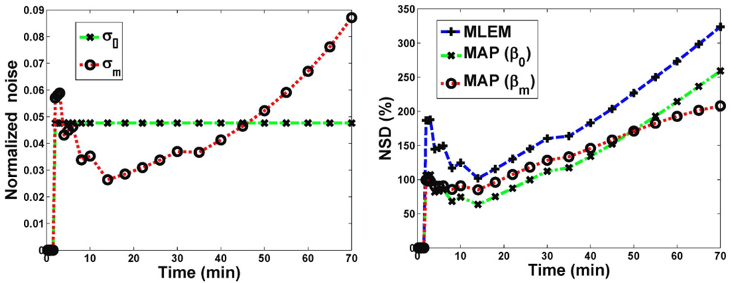
Figure 2(a) illustrates σ₀ and σ_k for a typical raclopride PET study. For a reasonable scaling factor α (as optimized in this study, as discussed later), the noise performance of QP-MAP reconstruction using frame-independent vs. frame-dependent regularization approaches is presented in figure 2(b). We can see that the latter approach utilizing frame-dependent β_k demonstrates enhanced uniformity across frames.

Figure 2.

(a) Comparison of σ₀ vs. σ_m as utilized in frame-independent vs. frame-dependent regularizations (13) and (11). To minimize dependence on early-uptake, highly-varying noise levels, only σ_m values for frames with t>1.5min were averaged to obtain σ₀, (b) Plots of resulting image NSD versus frame number for QP-MAP reconstruction using: (i) standard non-regularized MLEM shown as reference, (ii) QP-MAP with frame-independent regularization (MAP (β₀)), and (iii) QP-MAP with frame-dependent regularization (MAP (β_m)).

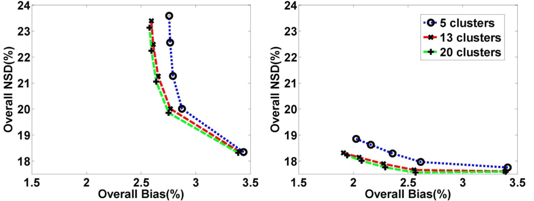
For the proposed 3.5D PET reconstruction method (including CP-W-MAP and CP-U-MAP), we also studied the impact of cluster number K on the quantitative accuracy, specifically by studying the final obtained parametric images. Through extensive testing, we found that within our task of parametric imaging in raclopride PET scans, use of 13 clusters provided reasonable results, as shown in figure 3.

Figure 3.

Plots of overall NSD (noise) vs. bias for DV images obtained with increasing iterations of 3.5D dynamic reconstruction: (left) CP-U-MAP and (right) CP-W-MAP for varying cluster numbers and using frame-dependent regularization with typical scaling factor α.

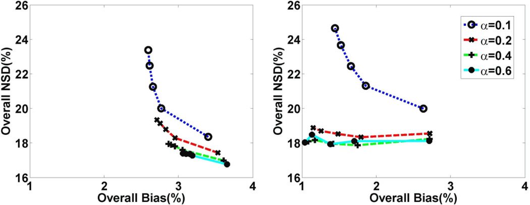
Next, the effect of varying the scaling factor α in the context of frame-dependent regularization was studied. We emphasize that optimization of regularization was performed for both conventional MAP (not shown) and proposed 3.5D MAP reconstruction (shown next), to provide a fair comparison between the two approaches. This was achieved using noise versus bias tradeoff curves as shown in figure 4. The curves in the plots (each generated with increasing iterations) demonstrate quantitatively improved overall NSD versus Bias trade-offs with increasing α values for both CP-U-MAP and CP-W-MAP reconstructions. Nonetheless, more notable quantitative improvements were observed for the latter: in fact, at a fixed iteration, both noise and bias levels were improved in CP-W-MAP, while in case of CP-U-MAP, reduced noise was obtained at the cost of degraded bias. This is attributed to the fact that CP-W-MAP reconstruction has an enhanced ability to minimize interactions between distant voxels that are incorrectly clustered together. As a result, in our subsequent work, we focus on this algorithm.

Figure 4.

Plots of overall NSD (noise) vs. bias for DV images obtained using proposed reconstruction method with 13 clusters: (left) CP-U-MAP and (right) CP-W-MAP, as generated for varying regularization parameters. Increasing bias levels were observed for CP-U-MAP reconstruction, unlike CP-W-MAP reconstruction.

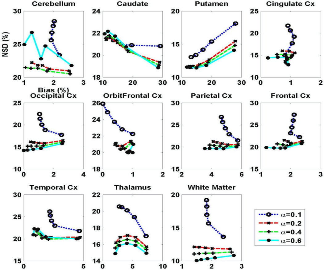
Figure 5 plots NSD versus Bias tradeoff curves for CP-W-MAP in representative individual brain regions as generated with increasing iterations, using different scaling factors α. For the α-values plotted, considerable improvements in image quality were achieved when α increased from 0.1 to 0.4 (increasing α to 0.6 did not noticeably impact performance). We thus utilized α=0.4 as an optimal value for CP-W-MAP reconstructions. Here, we wish to emphasize the practicality of optimizing α (and not β directly) allowing the regularization task to be naturally tuned for different scans given their unique overall or individual frame statistics, as pursued using equations (13) and (11) respectively, though we utilize the frame-dependent approach for enhanced performance.

Figure 5.

Plots of regional NSD (noise) vs. bias curves for DV images obtained using 3.5D dynamic reconstruction with 13 clusters (CP-W-MAP) for varying regularization parameter.

4.1.2. Results for the plasma input model

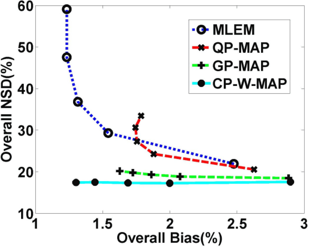
Following the optimization of parameters, we compared the performance of conventional 3D PET reconstructions (including MLEM, QP-MAP, GP-MAP) and proposed 3.5D PET reconstruction (CP-W-MAP). To provide an overall evaluation perfomance of the reconstruction algorithms across the brain, figure 6 depicts plots of overall NSD versus overall Bias for various parametric DV images. It is clearly seen that the MLEM approach results in substantially increasing noise levels with increasing iterations, while QP-MAP and GP-MAP approaches somewhat reduce the noise levels at the cost of degraded bias levels. By comparison, the proposed CP-W-MAP reconstruction method results in improved bias levels while controlling noise levels. It is also worth noting that GP-MAP performs better than QP-MAP in term of noise versus bias tradeoff of the reconstructed image.

Figure 6.

Plots of overall NSD (noise) vs. bias for DV images (generated with increasing iterations) obtained using: (i) conventional 3D MLEM reconstruction, (ii) conventional 3D MAP reconstruction (QP-MAP and GP-MAP) and (iii) proposed 3.5D reconstruction (CP-W-MAP). Regularization was optimized for both conventional and proposed MAP reconstructions to provide a fair comparison.

The regional NSD versus Bias tradeoffs (11 regions) of the DV images estimated from conventional 3D PET reconstruction (MLEM, QP-MAP and GP-MAP) and the proposed 3.5D PET reconstruction (CP-W-MAP) are shown in figure 7. As depicted in plots for the individual ROIs, applying conventional 3D MAP reconstruction can reduce the noise but sacrifices the bias. Noise versus bias tradeoff curves achieved by the proposed CP-W-MAP reconstruction method is seen to outperform those from MLEM and conventional MAP.

Figure 7.

Plots of regional NSD (noise) versus bias trade-off curves of the estimated DV images (generated with increasing iterations) for different regions of the brain reconstructed using (i) conventional 3D MLEM reconstruction, (ii) conventional 3D MAP reconstruction (QP-MAP and GP-MAP), and (iii) proposed 3.5D MAP reconstruction (CP-W-MAP)

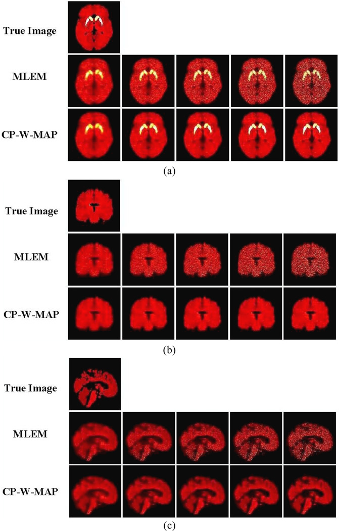
In order to provide a more direct visual impression of the estimated DV images, figure 8 shows transaxial, coronal, and sagittal slices through parametric images obtained by two algorithms (MLEM and CP-W-MAP), together with the true image. It is seen that while the standard MLEM approach results in increasingly noisy images (with increasing iterations), reconstructed images using the proposed CP-W-MAP approach show a clearly improved visual performance. Parametric images obtained by other two algorithms (QP-MAP and GP-MAP) are not shown in figure 8: both QP-MAP and especially GP-MAP reduced the noise levels though at the cost of degraded bias levels, the latter not easily detected visually, though clearly observed in quantitative noise versus bias analysis (e.g. figure 6 and figure 7).

Figure 8.

True and estimated parametric DV images: (a)–(c) corresponding to transaxial, coronal and sagittal slices, respectively. For each, (i) true image, (ii) standared 3D MLEM reconstruction (MLEM) and (iii) proposed 3.5D reconstruction (CP-W-MAP) are shown (From left to right): Increasing iterations of 1, 2, 3, 5 and 10 (16 subsets). No post-filtering was applied to the images shown.

4.1.3. Results for the reference input model

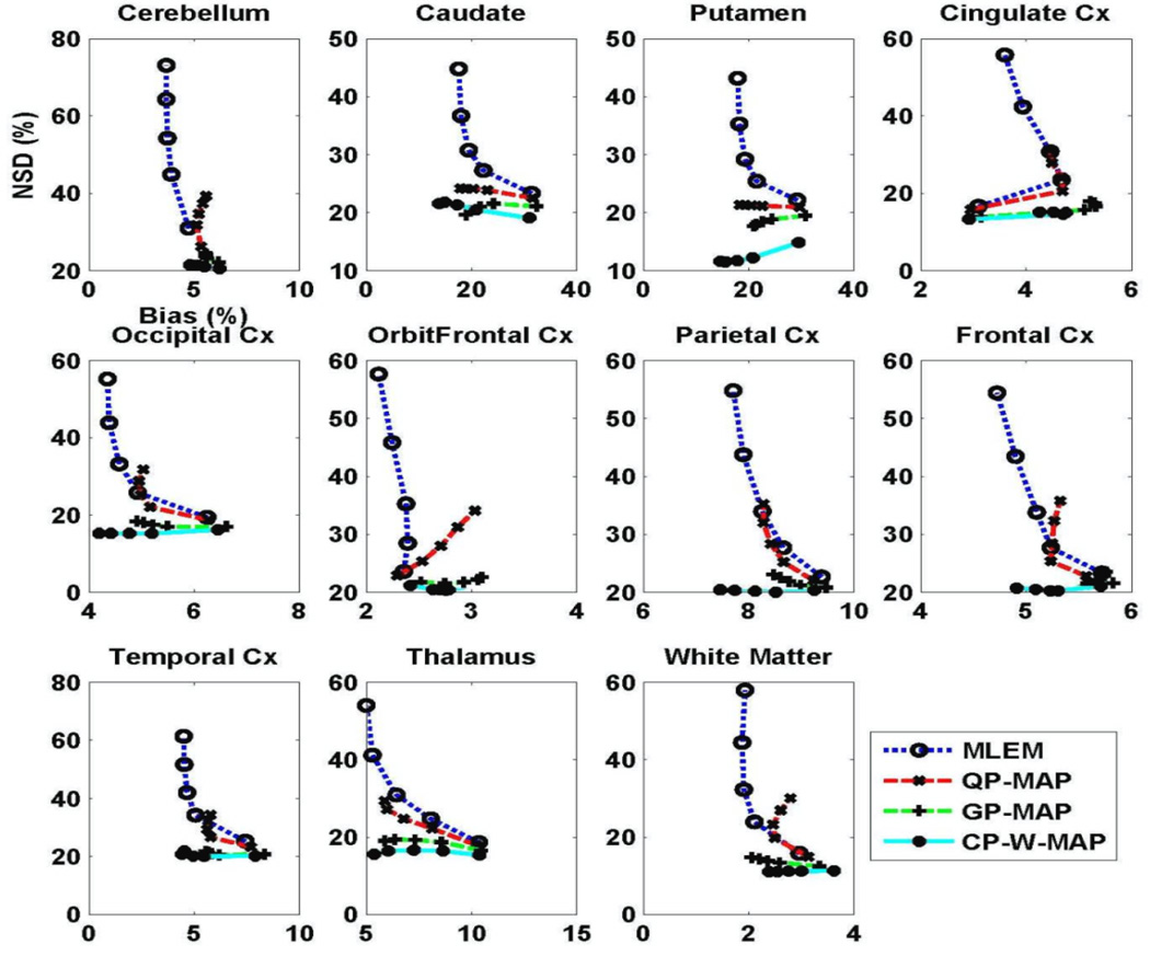
The abovementioned quantitative analysis was also performed on parametric DVR images obtained using the reference tissue model, with the cerebellum used as reference. Figure 9 shows regional NSD versus Bias tradeoffs (11 regions) of the DVR images estimated from conventional 3D PET reconstructions (MLEM, QP-MAP and GP-MAP) and the proposed 3.5D PET reconstruction method (CP-W-MAP). It is worth noting that for all reconstructions, the estimated parametric DVR images (obtained using the reference tissue model) lead to larger bias levels in comparison with using the plasma input model (figure 7). In any case, the proposed CP-W-MAP reconstruction method is seen to noticeably outperform conventional 3D reconstructions, by lowering the noise (NSD) while achieving reduced bias.

Figure 9.

Plots of regional NSD (noise) versus bias curves of the estimated DVR images (using the reference tissue model), as generated with increasing iteration numbers, for different regions of brain images reconstructed using (i) conventional 3D MLEM reconstruction, (ii) conventional 3D MAP reconstruction (MAP) and (iii) proposed 3.5D MAP reconstruction (CP-W-MAP).

4.2 Application to patient study

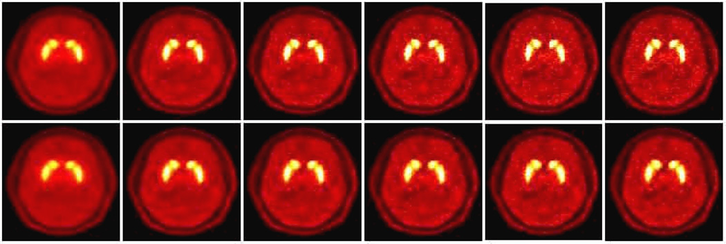
Subsequently, following extensive validations using simulations, we applied the proposed 3.5D reconstruction method to a ¹¹C-raclopride patient study on the HRRT scanner (as elaborated in section 3.2). In order to provide a visual comparison of the estimated DVR images, figure 10 shows transaxial slices of parametric images obtained by conventional MLEM and proposed 3.5D reconstruction algorithms. The noise reduction in parametric DVR image reconstructed from the proposed approach is clearly observed.

Figure 10.

Transaxial parametric DVR images for a raclopride HRRT study. (top) standared 3D MLEM reconstruction, (bottom) proposed 3.5D reconstruction (CP-W-MAP). (From left to right): Increasing iterations of 1, 2, 3, 4, 5 and 6 (16 subsets). Post-filtering was applied to the images shown.

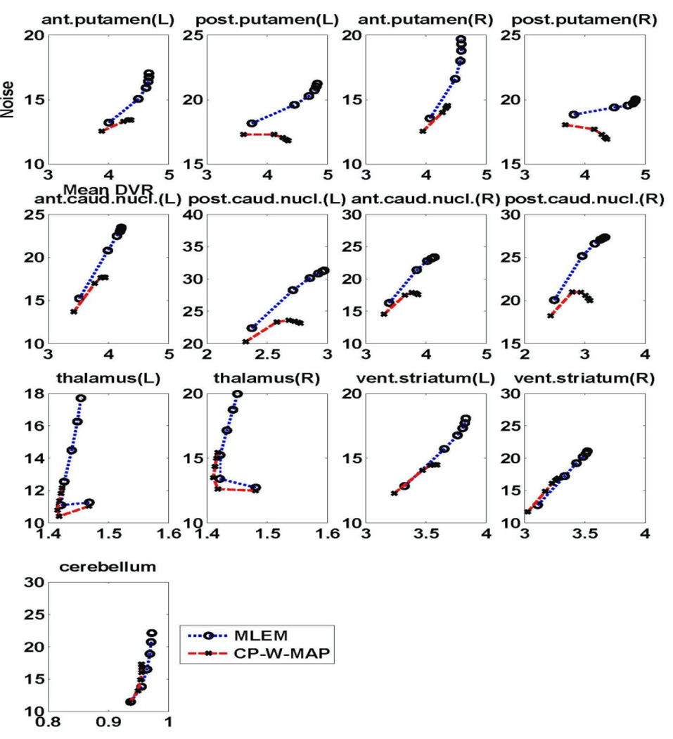
Figure 11 depicts Noise_ROI verus DVR_ROI plots generated by increasing iterations for 13 individual regions of the brain (cerebellum, both left (L) and right (R) anterior putamen, posterior putamen, anterior caudate nucleus, posterior caudate nucleus, thalamus and ventral striatum). Across these ROIs, the proposed 3.5D reconstruction method is commonly seen to quantitatively outperform conventional 3D MLEM reconstruction, in the sense that for a given DVR value, improved noise values are attained.

Figure 11.

Plots of regional NSD versus DVR curves of the estimated DVR images with the iteration number for different regions of brain images reconstructed using (i) standard 3D MLEM reconstruction, and (ii) proposed 3.5D MAP reconstruction (CP-W-MAP).

Future work consists of application to an extensive pool of test-retest subject studies on the HRRT scanner, aiming to validate a hypothesized enhanced quantitative accuracy using the proposed approach, including increased reproducibility (e.g. intraclass correlation coefficient (Shrout and Fleiss, 1979)).

5. Discussion

5.1. Relationship with spatiotemporal four-dimensional (4D) PET reconstruction

Spatiotemporal 4D PET reconstruction approaches, as reviewed in (Rahmim et al., 2009), aim to obtain improved noise performance for a given temporal sampling scheme, through incorporation of information from more than one frame in the reconstruction task. These include techniques that utilize (a) iterative temporal smoothing, (b) smooth temporal basis functions (c) principal components transformation of the dynamic data, (d) wavelet-based techniques and (e) direct kinetic parameter estimation methods. The direct approach, also reviewed in (Tsoumpas et al., 2008), combines kinetic modeling and emission image reconstruction into a single framework, comprehensively utilizing data from all dynamic frames in the reconstruction process. It allows accurate incorporation of noise from sinogram data within kinetic parameter estimation. However, this approach tends to require more complex optimization algorithms than conventional methods (Carson and Lange, 1985; Kamasak et al., 2005; Wang and Qi, 2009b). Though closed-form direct 4D parametric imaging algorithms have been developed, they are primarily based on linear graphical models (Wang et al., 2008; Tang et al., 2010; Rahmim et al., 2012). By comparison, while our proposed 3.5D dynamic PET reconstruction does extract and incorporate 4D kinetics information from the overall data, it maintains a straightforward approach to 3D reconstruction of individual frames, and does not require the use of temporal basis functions, complex transforms or sophisticated optimization algorithms. Furthermore, the algorithm does not require pre-specification of the kinetic model to be applied to the reconstructed images.

5.2. Selection of cluster number

The true number of clusters is usually not known a priori. Therefore one faces the challenge of specifying the appropriate number of clusters. In the work by Belhassen and Zaidi (Belhassen and Zaidi, 2010), the number of clusters for a static PET image is computed by optimizing the Bayesian information criterion (BIC). Wong et al (Wong et al., 2002) used two information theoretic criteria, namely the Akaike information criterion (AIC) and the Schwaz criterion (SC, which is equivalent to BIC) to determine the number of clusters for 2D dynamic PET images. AIC and BIC invoke different statistical models (Schwarz, 1978). Nonetheless, in our simulations, we did not find AIC and BIC to perform reliably for realistic 3D dynamic PET images. One possible reason is that both AIC and BIC are model dependent, thus a specific probability distribution function is not appropriate for the realistic 3D dynamic PET images.

In this study, we have instead used quantitative NSD versus Bias tradeoff performance to optimize the cluster number. We previously studied the effect of different cluster numbers on static image reconstruction (Lu et al., 2011). It was found that if the cluster number is less than the true number of clusters, reconstructed images obtained using CP-U-MAP may introduce notable bias, while CP-W-MAP depicted better performance: this was attributed to the ability of CP-W-MAP to minimize interactions between distant voxels that may have been wrongly clustered together. This was also validated in the present context of dynamic imaging: the overall NSD versus Bias tradeoff curves for parametric images obtained following CP-W-MAP reconstruction depicted enhanced quantitative performance compared to CP-U-MAP reconstruction when the number of clusters was set to less than the true number of clusters (as illustrated in Section 4.1.1; figure 3). We also observed neither obvious improvements nor degradations in overall NSD versus Bias tradeoff performance when the number of clusters was greater than the true number of clusters (i.e. 13). However, as the true number of clusters is not known in practice and underestimation is expected to lead to poor quantitative performance, it may be wiser to follow an aggressive approach that is more likely to induce over- rather than underestimation of this parameter. Alternatively, it is possible to explore approaches such as hierarchical cluster analysis (Huang et al., 2007) to fit the dynamic data using a varying number of clusters until an optimum value is reached.

5.3. Selection of the regularization parameter

Selection of a proper regularization parameter β in MAP reconstruction can be critical for dynamic PET reconstructions. Adaptive approaches such as generalized cross validation (GCV), L-curve and maximum likelihood methods (Johnson et al., 1991; Saquib et al., 1998; Zhou et al., 1997; Hansen, 1992) impose high computational costs and are not task-based. Wang and Qi proposed a kinetic-task-dependent method to guide the selection of regularization parameters in the MAP reconstruction for dynamic PET (Wang and Qi, 2009a). However, this method, aside from its computational complexity, requires both the estimated true value of the TAC inside the ROI and the definition of the ROI (prompting ‘plug-in’ approaches). In the present work, given the dependence of both image resolution and noise levels on frame statistics (Qi and Leahy, 2000), we utilized a simple yet practical approach of scaling the regularization parameters in accordance with the variance of each dynamic frame (as elaborated in Section 2.3). We used NSD versus Bias tradeoff curves to optimize the scaling factor, and demonstrated more uniform noise levels (NSD) between the reconstructed images from the various dynamic frames.

6. Summary

This work proposed a 3.5D dynamic PET reconstruction method to enhance the image reconstruction via introduction of priors based on voxel kinetics. We used a weighted fuzzy C-means method to cluster the preliminary reconstructed dynamic images and then defined neighborhoods of voxels with similar kinetics. Two forms of cluster-based priors were defined and incorporated via straightforward maximum a posterior (MAP) 3D PET reconstruction as applied to individual frames. Using realistic simulated ¹¹C-raclopride dynamic PET data, we optimize the performance of the proposed 3.5D dynamic PET reconstruction algorithm, and compared its performance with conventional 3D MLEM and MAP (QP-MAP and GP-MAP) reconstruction algorithms. A frame-dependent regularization parameter was developed and studied quantitatively, using overall NSD versus frame, to obtain relative consistency in image resolution and noise amongst different frames. The proposed 3.5D dynamic reconstruction algorithm resulted in quantitatively enhanced DV and DVR parametric images, as demonstrated in extensive ¹¹C-raclopride PET simulation as well as an HRRT patient study.

References

- Ahmed MN, Yamany SM, Mohamed N, Farag AA, Moriarty T. A modified fuzzy C-means algorithm for bias field estimation and segmentation of MRI data. IEEE Trans. Med. Imaging. 2002;21:193–199. doi: 10.1109/42.996338. [DOI] [PubMed] [Google Scholar]
- Anzai Y, Minoshima S, Wolf GT, Wahl RL. Head and neck cancer: detection of recurrence with three-dimensional principal components analysis at dynamic FDG PET. Radiology. 1999;212:285–290. doi: 10.1148/radiology.212.1.r99jl02285. [DOI] [PubMed] [Google Scholar]
- Baete K, Nuyts J, Van Paesschen W, Suetens P, Dupont P. Anatomical-based FDG-PET reconstruction for the detection of hypo-metabolic regions in epilepsy. IEEE Trans. Med. Imaging. 2004;23:510–519. doi: 10.1109/TMI.2004.825623. [DOI] [PubMed] [Google Scholar]
- Belhassen S, Zaidi H. A novel fuzzy C-means algorithm for unsupervised heterogeneous tumor quantification in PET. Med. Phys. 2010;37:1309–1324. doi: 10.1118/1.3301610. [DOI] [PubMed] [Google Scholar]
- Bentourkia M, Zaidi H. Tracer kinetic modeling in PET. PET Clin. 2007;2:267–277. doi: 10.1016/j.cpet.2007.08.003. [DOI] [PubMed] [Google Scholar]
- Bezdek JC. Pattern recognition with fuzzy objective function algorithms. New York: Plenum; 1981. [Google Scholar]
- Carson RE, Lange K. The EM parametric image reconstruction algorithm. J. Am. Stat. Assoc. 1985;80:20–22. [Google Scholar]
- Chen S, Zhang D. Robust image segmentation using FCM with spatial constraints based on new kernel-induced distance measure. IEEE Trans. Syst., Man, Cybern. 2004;34:1907–1916. doi: 10.1109/tsmcb.2004.831165. [DOI] [PubMed] [Google Scholar]
- Comtat C, Kinahan PE, Fessler JA, Beyer T, Townsend DW, Defrise M, Michel C. Clinically feasible reconstruction of 3D whole-body PET/CT data using blurred anatomical labels. Phys. Med. Biol. 2002;47:1–20. doi: 10.1088/0031-9155/47/1/301. [DOI] [PubMed] [Google Scholar]
- El Fakhri G, Sitek A, Guérin B, Kijewski MF, Di Carli MF, Moore SC. Quantitative dynamic cardiac 82Rb PET using generalized factor and compartment analyses. J. Nucl. Med. 2005;46:1264–1271. [PubMed] [Google Scholar]
- Geman S, McClure DE. Statistical methods for tomographic image reconstruction IS1 Tokyo session. Bull. Int. Stat. Inst. 1987;LII-4:5–21. [Google Scholar]
- Geman S, Geman D. Stochastic relaxation, Gibbs distributions, and the Bayesian restoration of images. IEEE Trans. Pattern Anal. Mach. Intell. 1984;6:721–741. doi: 10.1109/tpami.1984.4767596. [DOI] [PubMed] [Google Scholar]
- Green PJ. Bayesian reconstructions from emission tomography data using a modified EM algorithm. IEEE Trans. Med. Imaging. 1990;9:84–93. doi: 10.1109/42.52985. [DOI] [PubMed] [Google Scholar]
- Hansen PC. Analysis of discrete ill-posed problems by means of the L-curve. SIAM Rev. 1992;34:561–580. [Google Scholar]
- Hsiao I, Rangarajan A, Gindi G. A new convex edge-preserving median prior with applications to tomography. IEEE Trans. Med. Imaging. 2003;22:580–585. doi: 10.1109/TMI.2003.812249. [DOI] [PubMed] [Google Scholar]
- Huang X, Zhou Y, Bao S, Huang SC. Clustering-based linear least square fitting method for generation of parametric images in dynamic FDG PET studies. J. Biomed. Imag. 2007;2007:1–12. doi: 10.1155/2007/65641. [DOI] [PMC free article] [PubMed] [Google Scholar]
- Innis RB, Cunningham VJ, Delforge J, Fujita M, Gjedde A, Gunn RN, Holden J, Houle S, Huang SC, Ichise M. Consensus nomenclature for in vivo imaging of reversibly binding radioligands. J. Cereb. Blood Flow Metab. 2007;27:1533–1539. doi: 10.1038/sj.jcbfm.9600493. [DOI] [PubMed] [Google Scholar]
- Janssen MH, Aerts HJ, Ollers MC, Bosmans G, Lee JA, Buijsen J, De Ruysscher D, Lambin P, Lammering G, Dekker AL. Tumor delineation based on time-activity curve differences assessed with dynamic fluorodeoxyglucose positron emission tomography-computed tomography in rectal cancer patients. Int. J. Radiat. Oncol. Biol. Phys. 2009;73:456–465. doi: 10.1016/j.ijrobp.2008.04.019. [DOI] [PubMed] [Google Scholar]
- Johnson VE, Wong WH, Hu X, Chen CT. Image restoration using Gibbs priors: Boundary modeling, treatment of blurring, and selection of hyperparameter. IEEE Trans. Pattern Anal. Mach. Intell. 1991;13:413–425. [Google Scholar]
- Kamasak ME, Bouman CA, Morris ED, Sauer K. Direct reconstruction of kinetic parameter images from dynamic PET data. IEEE Trans. Med. Imaging. 2005;24:636–650. doi: 10.1109/TMI.2005.845317. [DOI] [PubMed] [Google Scholar]
- Kimura Y, Hsu H, Toyama H, Senda M, Alpert NM. Improved signal-to-noise ratio in parametric images by cluster analysis. Neuroimage. 1999;9:554–561. doi: 10.1006/nimg.1999.0430. [DOI] [PubMed] [Google Scholar]
- Kimura Y, Noshi Y, Oda K, Ishii K. Formation of parametric images in positron emission tomography using a clustering-based kinetic analysis with statistical clustering. IEEE Proc. 23 rd Annual EMBS Int. Conf. 2001;3:2763–2765. [Google Scholar]
- Kimura Y, Senda M, Alpert NM. Fast formation of statistically reliable FDG parametric images based on clustering and principal components. Phys. Med. Biol. 2002;47:455–468. doi: 10.1088/0031-9155/47/3/307. [DOI] [PubMed] [Google Scholar]
- Koivistoinen H, Tohka J, Ruotsalainen U. Comparison of pattern classification methods in segmentation of dynamic PET brain images; Proc. of the 6th Nordic Signal Processing Symp. (NORSIG 2004); 2004. pp. 73–76. [Google Scholar]
- Leahy RM, Qi J. Statistical approaches in quantitative positron emission tomography. Stat. Comput. 2000;10:147–165. [Google Scholar]
- Lipinski B, Herzog H, Rota Kops E, Oberschelp W, Muller-Gartner HW. Expectation maximization reconstruction of positron emission tomography images using anatomical magnetic resonance information. IEEE Trans. Med. Imaging. 1997;16:129–136. doi: 10.1109/42.563658. [DOI] [PubMed] [Google Scholar]
- Liptrot M, Adams KH, Martiny L, Pinborg LH, Lonsdale MN, Olsen NV, Holm S, Svarer C, Knudsen GM. Cluster analysis in kinetic modelling of the brain: a noninvasive alternative to arterial sampling. Neuroimage. 2004;21:483–493. doi: 10.1016/j.neuroimage.2003.09.058. [DOI] [PubMed] [Google Scholar]
- Lu L, Tang J, Karakatsanis N, Chen W, Rahmim A cluster-based priors for MAP PET image reconstruction; IEEE Nucl. Sci. Symp. Med. Imaging Conf. Rec; 2011. pp. 2678–2681. 2011. [Google Scholar]
- Mumcuoğlu EU, Leahy RM, Cherry SR. Bayesian reconstruction of PET images: methodology and performance analysis. Phys. Med. Biol. 1996;41:1777–1807. doi: 10.1088/0031-9155/41/9/015. [DOI] [PubMed] [Google Scholar]
- Nuyts J, Beque D, Dupont P, Mortelmans L. A concave prior penalizing relative differences for maximum-a-posteriori reconstruction in emission tomography. IEEE Trans. Nucl. Sci. 2002;49:56–60. [Google Scholar]
- Qi J, Leahy RM. Resolution and noise properties of MAP reconstruction for fully 3-D PET. IEEE Trans. Med. Imaging. 2000;19:493–506. doi: 10.1109/42.870259. [DOI] [PubMed] [Google Scholar]
- Rahmim A, Zaidi H. PET versus SPECT: strengths, limitations and challenges. Nucl. Med. Commun. 2008;29:193–207. doi: 10.1097/MNM.0b013e3282f3a515. [DOI] [PubMed] [Google Scholar]
- Rahmim A, Cheng JC, Blinder S, Camborde ML, Sossi V. Statistical dynamic image reconstruction in state-of-the-art high-resolution PET. Phys. Med. Biol. 2005;50:4887–4912. doi: 10.1088/0031-9155/50/20/010. [DOI] [PubMed] [Google Scholar]
- Rahmim A, Dinelle K, Cheng JC, Shilov MA, Segars WP, Lidstone SC, Blinder S, Rousset OG, Vajihollahi H, Tsui B. Accurate event-driven motion compensation in high-resolution PET incorporating scattered and random events. IEEE Trans. Med. Imaging. 2008;27:1018–1033. doi: 10.1109/TMI.2008.917248. [DOI] [PMC free article] [PubMed] [Google Scholar]
- Rahmim A, Tang J, Zaidi H. Four-dimensional (4D) image reconstruction strategies in dynamic PET: Beyond conventional independent frame reconstruction. Med. Phys. 2009;36:3654–3670. doi: 10.1118/1.3160108. [DOI] [PubMed] [Google Scholar]
- Rahmim A, Zhou Y, Tang J, Lu L, Sossi V, Wong DF. Direct 4D parametric imaging for linearized models of reversibly binding PET tracers using generalized AB-EM reconstruction. Phys. Med. Biol. 2012;57:733–755. doi: 10.1088/0031-9155/57/3/733. [DOI] [PMC free article] [PubMed] [Google Scholar]
- Rangarajan A, Hsiao IT, Gindi G. A Bayesian joint mixture framework for the integration of anatomical information in functional image reconstruction. J. Math. Imaging Vis. 2000;12:199–217. [Google Scholar]
- Reader AJ, Zaidi H. Advances in PET image reconstruction. PET Clin. 2007;2:173–190. doi: 10.1016/j.cpet.2007.08.001. [DOI] [PubMed] [Google Scholar]
- Saquib SS, Bouman CA, Sauer K. ML parameter estimation for Markov random fields with applications to Bayesian tomography. IEEE Trans. Image Process. 1998;7:1029–1044. doi: 10.1109/83.701163. [DOI] [PubMed] [Google Scholar]
- Schwarz G. Estimating the dimension of a model. Ann. Stat. 1978;6:461–464. [Google Scholar]
- Shrout PE, Fleiss JL. Intraclass correlations: uses in assessing rater reliability. Psychol. Bull. 1979;86:420–428. doi: 10.1037//0033-2909.86.2.420. [DOI] [PubMed] [Google Scholar]
- Somayajula S, Panagiotou C, Rangarajan A, Li Q, Arridge SR, Leahy RM. PET image reconstruction using information theoretic anatomical priors. IEEE Trans. Med. Imaging. 2011;30:537–549. doi: 10.1109/TMI.2010.2076827. [DOI] [PMC free article] [PubMed] [Google Scholar]
- Sossi V, et al. The second generation HRRT-a multi-centre scanner performance investigation; IEEE Nuclear Science Symp. Conf. Record; 2005. pp. 2195–2199. 2005. [Google Scholar]
- Tang J, Rahmim A. Bayesian PET image reconstruction incorporating anato-functional joint entropy. Phys. Med. Biol. 2009;54:7063–7075. doi: 10.1088/0031-9155/54/23/002. [DOI] [PMC free article] [PubMed] [Google Scholar]
- Tang J, Kuwabara H, Wong DF, Rahmim A. Direct 4D reconstruction of parametric images incorporating anato-functional joint entropy. Phys. Med. Biol. 2010;55:4261–4272. doi: 10.1088/0031-9155/55/15/005. [DOI] [PMC free article] [PubMed] [Google Scholar]
- Tsoumpas C, Turkheimer FE, Thielemans K. A survey of approaches for direct parametric image reconstruction in emission tomography. Med. Phys. 2008;35:3963–3971. doi: 10.1118/1.2966349. [DOI] [PubMed] [Google Scholar]
- Vunckx K, Atre A, Baete K, Reilhac A, Deroose C, Van Laere K, Nuyts J. Evaluation of three MRI-based anatomical priors for quantitative PET brain imaging. IEEE Trans. Med. Imaging. 2011;31:599–612. doi: 10.1109/TMI.2011.2173766. [DOI] [PubMed] [Google Scholar]
- Wang G, Qi J. Analysis of penalized likelihood image reconstruction for dynamic PET quantification. IEEE Trans. Med. Imaging. 2009a;28:608–620. doi: 10.1109/TMI.2008.2008971. [DOI] [PMC free article] [PubMed] [Google Scholar]
- Wang G, Qi J. Generalized algorithms for direct reconstruction of parametric images from dynamic PET data. IEEE Trans. Med. Imaging. 2009b;28:1717–1726. doi: 10.1109/TMI.2009.2021851. [DOI] [PMC free article] [PubMed] [Google Scholar]
- Wang G, Fu L, Qi J. Maximum a posteriori reconstruction of the Patlak parametric image from sinograms in dynamic PET. Phys. Med. Biol. 2008;53:593–604. doi: 10.1088/0031-9155/53/3/006. [DOI] [PubMed] [Google Scholar]
- Wong KP, Feng D, Meikle SR, Fulham MJ. Segmentation of dynamic PET images using cluster analysis. IEEE Trans. Nucl. Sci. 2002;49:200–207. [Google Scholar]
- Yaqub M, Boellaard R, Kropholler MA, Lammertsma AA. Optimization algorithms and weighting factors for analysis of dynamic PET studies. Phys. Med. Biol. 2006;51:4217–4232. doi: 10.1088/0031-9155/51/17/007. [DOI] [PubMed] [Google Scholar]
- Zhou Y, Huang SC, Bergsneider M, Wong DF. Improved parametric image generation using spatial-temporal analysis of dynamic PET studies. Neuroimage. 2002;15:697–707. doi: 10.1006/nimg.2001.1021. [DOI] [PubMed] [Google Scholar]
- Zhou Y, Ye W, Brasić JR, Crabb AH, Hilton J, Wong DF. A consistent and efficient graphical analysis method to improve the quantification of reversible tracer binding in radioligand receptor dynamic PET studies. Neuroimage. 2009;44:661–670. doi: 10.1016/j.neuroimage.2008.09.021. [DOI] [PMC free article] [PubMed] [Google Scholar]
- Zhou Z, Leahy RN, Qi J. Approximate maximum likelihood hyperparameter estimation for Gibbs priors. IEEE Trans. Image Process. 1997;6:844–861. doi: 10.1109/83.585235. [DOI] [PubMed] [Google Scholar]