Elucidating the Locking Mechanism of Peptides onto Growing Amyloid Fibrils through Transition Path Sampling

Abstract

We investigate the molecular mechanism of monomer addition to a growing amyloid fibril composed of the main amyloidogenic region from the insulin peptide hormone, the $LVEALYL$ heptapeptide. Applying transition path sampling in combination with reaction coordinate analysis reveals that the transition from a docked peptide to a locked, fully incorporated peptide can occur in two ways. Both routes involve the formation of backbone hydrogen bonds between the three central amino acids of the attaching peptide and the fibril, as well as a reorientation of the central Glu side chain of the locking peptide toward the interface between two β-sheets forming the fibril. The mechanisms differ in the sequence of events. We also conclude that proper docking is important for correct alignment of the peptide with the fibril, as alternative pathways result in misfolding.

Introduction

Amyloid fibrils are highly ordered protein or polypeptide assemblies that are best known in connection with neurodegenerative diseases like Alzheimer’s and Parkinson’s (1,2). More recently, however, a number of naturally occurring fibril-forming proteins with functional rather than disease-related properties have been discovered (3–5). In addition, such peptides may be attractive building blocks for self-assembling nanomaterials (6,7).

The formation of amyloid fibers is not well understood, but it involves several steps. The first step is a nucleation event in which peptides aggregate into oligomers; this is followed by a transition to a small, ordered seed. This seed can grow, fragment, or provide a template for secondary nucleation (8). Subsequent amyloid fibril growth is thought to occur through incorporation of sequential peptide monomers (9). This monomer addition is essentially a two-step process, often referred to as a dock-lock mechanism, which can be written as the reaction ${\text{P}}^{\text{S}}\rightleftharpoons {\text{P}}^{\text{D}}\rightleftharpoons {\text{P}}^{\text{F}}$, where ${\text{P}}^{\text{S}}$, ${\text{P}}^{\text{D}}$, and ${\text{P}}^{\text{F}}$ represent the peptide in solution, in the docked state, and in the fibril state, respectively. In the first step, the fully solvated monomer docks on an existing fibril seed by weakly binding to it. In the ${\text{P}}^{\text{D}}\rightleftharpoons {\text{P}}^{\text{F}}$ step, the monomer adopts the conformation of the peptides in the fibril, thereby enhancing its binding affinity for the fibril (9–14). During this so-called locking phase, backbone hydrogen bonds between the peptide and the fibril form, and a dry interface between the sheets appears. Such a dry interface is often called a steric zipper (15). Although both steps are in principle reversible, the second step is in fact shifted toward ${\text{P}}^{\text{F}}$, so that ${\text{P}}^{\text{D}}\to {\text{P}}^{\text{F}}$ is usually considered irreversible.

The docking step occurs on a timescale ${\tau }_D$, and locking takes place on timescale ${\tau }_L$. Estimates from experiments (11) and simulation (16) have shown that ${\tau }_L/{\tau }_D\gg 1$ at experimentally relevant concentrations. Hence, locking is the rate-limiting step in monomer addition.

In this work, we aim to study the dynamical mechanism of addition of a heptapeptide to a growing fibril. This will give further insight into the growth mechanism and might eventually lead to the rational design of inhibitors of amyloid formation (8). Short peptides have been studied extensively as model systems for their full-length proteins, both experimentally and with computer simulation, as they are more convenient to work with. Moreover, such peptides can be easily synthesized and modified, making them attractive building blocks for nanomaterials (6). Knowledge of the interactions involved in docking and locking of the peptides onto growing fibrils would also benefit the rational design of such peptide building blocks.

As our model system we chose the amyloidogenic heptapeptide ${}^{11}\text{LVEALYL}^{17}$ from the insulin B-chain. The full-length peptide hormone insulin consists of two chains linked by two disulfide bridges. Insulin fibril formation is enhanced at elevated temperatures, low pH, and increased ionic strength (17–19). Fibril formation causes problems in the production and storage of insulin for pharmaceutical purposes (20). Moreover, insulin fibrils have been observed at sites of frequent insulin injection in patients suffering from diabetes (21,22). The ${}^{11}\text{LVEALYL}^{17}$ sequence from the B-chain has been identified as the culprit in insulin fibril formation, and a high-resolution structure has been recently elucidated (23). The atomistic, dynamical mechanism of fibril formation, however, remains a mystery.

In principle, it is possible to use straightforward molecular dynamics (MD) simulations to study the kinetic mechanism of monomer addition to a growing fibril end (12–14). However, this approach is inefficient, as the simulation will spend a long time sampling the (meta)stable states. Moreover, observation of a single event will not be conclusive, as conformational changes can occur via many different pathways. Thus, the use of straightforward MD simulations to study spontaneous peptide docking and locking would be computationally very expensive. Many rare event sampling methods have been developed to overcome the large timescales inherent in straightforward MD simulations. These methods, however, rely either on biasing the system along a predefined reaction coordinate (e.g., steered MD (SMD) (24), umbrella sampling (25), or metadynamics (26)) or on acceleration of the dynamics by raising the temperature, known as replica-exchange MD (REMD) (27). As the choice of order parameter in which to bias can severely affect the reaction pathway, true insight into the kinetic mechanism can only be obtained from unbiased MD simulations. On the other hand, although the correct kinetic information for the dynamics at ambient temperature can in principle be extracted from REMD simulations (28), transitions observed in REMD simulations usually occur at high temperatures and may therefore not be representative of the mechanism at ambient temperature. Transition path sampling (TPS) (29) enables the collection of an ensemble of unbiased reactive trajectories that connect one (meta)stable state to another at the temperature of interest. These reactive trajectories are relatively short (in the order of nanoseconds), whereas conventional MD simulations would require several micro- to milliseconds to obtain a similar sampling of transitions. The path ensemble resulting from a TPS simulation allows the evaluation of the mechanisms and the transition-state ensemble (29), as well as optimization of the reaction coordinate (30). Here, we employ TPS simulations to elucidate the kinetic mechanism of the rate-limiting locking step of a peptide monomer to an amyloid fibril. To bootstrap the TPS simulation, we generated an initial path using SMD. Although it is also possible to generate an initial path from, for instance, a high-temperature simulation, an SMD path is more likely to be close to an unbiased low-temperature transition path, provided that a low velocity is used in the constant-velocity pulling scheme. Analysis of the resulting path ensemble yields insight into the reaction mechanism. Moreover, likelihood maximization (30,31) provides an optimized reaction coordinate to describe the progress of the fibril growth reaction.

Methods

System preparation

To keep the TPS simulations tractable, we constructed a small fibril seed consisting of a stack of two interdigitated parallel β-sheets of four peptides with sequence ${\text{LVEALYL}}^{17}$, based on the crystal structure PDB code 3HYD (23). For clarity, we will refer to the sheets as SH1 and SH2, with the peptides numbered per sheet (SH1P1–SH1P4) and the residues numbered per peptide (SH1P1L1), as indicated in Fig. 1. This system will henceforth be referred to as the fibril. The fibril belongs to class 1 (15), which is characterized by a stack of parallel β-sheets, with the sheets oriented such that the same residues interact to form the interface (referred to as face-to-face orientation) and having the same edge of their strands facing up (referred to as up-up). The peptides are simulated using the GROMOS96 force field (32) and are solvated by simple point charge (SPC) water molecules (33). The GROMOS96 force field was shown previously to give the best representation of experimentally observed dynamical behavior of the insulin B-chain (34). As fibril formation is most pronounced at low pH, the glutamate side chains and the N- and C-termini of the peptides are protonated. The system is neutralized by eight Cl⁻ ions.

Figure 1.

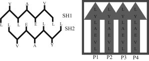
Schematic side and top view of the fibril. Amino acids are indicated by L, leucine (Leu); V, valine (Val); E, glutamate (Glu); A, alanine (Ala); and Y, tyrosine (Tyr). The sheets are labeled SH1 and SH2, and the peptides within one sheet are labeled P1–P4. Hence, SH1P2 refers to peptide 2 of sheet 1. The side view indicates which amino acid side chains interact to form the dry interface between the sheets. As shown in the top view, peptides form parallel β-sheets.

All simulations are performed with the GROMACS package version 4.0 (35). Using constraints—LINCS (36) for the protein and SETTLE (37) for the water molecules—allows for a 2-fs time step. The temperature is kept constant at 311 K using the velocity-rescale thermostat (38).

The solvated fibril system, measuring 5 × 5 × 5 nm³ and containing 4005 SPC waters, was energy-minimized using conjugate gradient and a 20-ps simulation with position restraints on the protein was run to equilibrate the water around the fibril. For this simulation, the pressure is kept at 1 bar using Parrinello-Rahman coupling (39). A 50-ns straightforward MD simulation was performed to test the fibril’s stability. The resulting structure is used as input for the SMD simulations.

SMD simulation

SMD creates nonequilibrium trajectories by pulling along a predefined coordinate to force a transition (24,40). The SMD simulations are performed in a rectangular box (4 × 4 × 7 nm³, 3432 SPC waters, volume adjusted to the average volume after equilibration) at constant volume (after energy minimization and water equilibration as described above). The sheets are oriented such that the hydrogen bonds align with the long axis of the box (the z axis). One of the outer peptides (SH1P1) was pulled away from the fibril along the z axis (pulling velocity, v = 0.31 nm/ns; spring constant, k =10,000 kJ/mol nm²), leaving a stepwise vacancy in the fibril, with one sheet consisting of four peptides and one sheet consisting of three peptides (see Fig. 3.). The pulling was done on the center of mass (COM) of the backbone atoms of SH1P1 with respect to the COM of the backbone atoms of the remaining peptides in the fibril. The other peptides in the fibril are position-restrained (by applying a harmonic potential of 1000 kJ/mol nm² to the backbone atoms) to prevent the detachment of other peptides (14).

Figure 3.

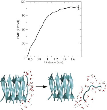
(Upper) PMF obtained from 20 SMD simulations. (Lower) Start and end configurations of one of the SMD simulations. The free energy difference between these states is ∼110 kJ/mol.

Twenty individual SMD trajectories (3.5 ns/trajectory) were generated to calculate the probability mass function (PMF) for removing one peptide from the fibril. The PMF was calculated according to Jarzynski’s relation (41) using the stiff-spring approach (24,40). In this limit, one can use the second cumulant expression (24,40).

The SMD trajectory with the lowest dissipation was used as the initial trajectory for the TPS simulations.

Transition path sampling

TPS samples the ensemble of paths connecting two predefined stable states, A and B, by performing a Monte Carlo random walk through trajectory space (29). Order parameters are only needed to define the stable states, whereas the paths themselves are dynamically unbiased, in contrast to paths obtained with, e.g., SMD or metadynamics (26). The TPS simulation needs to be bootstrapped with an initial path that we obtained from the SMD simulations. Although it is also possible to generate an initial path by a high-temperature simulation, in practice such paths require longer equilibration times compared to initial paths created by SMD or metadynamics. The latter paths are more likely to be close to an unbiased low-temperature transition path, provided one uses a low-velocity pulling protocol in the SMD. From the initial path, new trial paths are generated using a one-way shooting algorithm with flexible path length (42–44). The velocity-rescale thermostat ensures the stochastic nature of the MD trajectories. The sampling of the path ensemble was done using a perl script wrapper around the GROMACS package. We note that the resulting path ensemble represents the equilibrium path ensemble between A and B (29,45). Therefore, the pathways can be interpreted in terms of the equilibrium dissociation process as well as the association process.

Reaction-coordinate analysis

Transition path theory states that a good reaction coordinate can predict the committor $p_B\left(x\right)$ (46,47). The committor, also known as splitting probability or p-fold, is the probability that a trajectory started from a configuration x with randomized momenta reaches the final state, B, before reaching the initial state, A. Committor analysis can test whether a trial reaction coordinate is a good reaction coordinate, but is computationally exceedingly expensive, as it requires full committor distributions. The likelihood maximization (LM) method developed by Peters et al. (30,31) allows a reaction-coordinate analysis requiring data using the TPS simulation only. These data consist of the ensemble of forward (or backward) shooting-point configurations belonging to accepted trajectories (going to the final state, B) and the rejected shooting points (returning to the initial state, A). The LM method searches for the optimal reaction coordinate, $r\left(q\right)$, by screening all possible linear combinations of a predefined set of trial collective variables, q. To do so, the method optimizes the likelihood

$$L=\prod _{x_{sp}\to B}{p}_B\left(r\left(x_{sp}\right)\right)\prod _{x_{sp}\to A}\left(1-p_B\left(r\left(x_{sp}\right)\right)\right),$$ (1)

where the products run over the shooting points, $x_{sp}$, in the data set that lead to A or B, respectively. The committor $p_B\left(r\left(x\right)\right)$ is the model function to which the data are fitted:

$$p_B\left(r\left(x\right)\right)=\frac{1}{2}+\frac{1}{2}\text{tanh}\left(r\left[q\left(x\right)\right]\right),$$ (2)

where the trial reaction coordinate $r\left(q\left(x\right)\right)$ is a linear combination of order parameters $q_i$ :

$$r\left(q\left(x\right)\right)=\sum _{i=1}^n{a}_i{q}_i\left(x\right)+a_0,$$ (3)

where $a_i$ are the coefficients to be optimized by the LM method. The (nonlinear) optimization itself is done using the Broyden-Fletcher-Goldfarb-Shanno method, as described in Peters and Trout (30).

This reaction-coordinate analysis allows the screening of many combinations of collective variables as trial reaction coordinates. The linear combination of order parameters with the largest likelihood reproduces the shooting-point data best, and is thus the optimal reaction coordinate. For each shooting point in the ensemble we computed all the collective variables listed in Table 1. Employing the LM approach, we tested all possible linear combinations of up to three order parameters and kept the ones with the maximum likelihood as our best model for the reaction coordinate.

Table 1.

Overview of the order parameters monitored during the TPS simulations

OP name	Description
dL1L	Cα distance SH1P1L1–SH1P2L1
dV2V	Cα distance SH1P1V2–SH1P2V2
dE3E	Cα distance SH1P1E3–SH1P2E3
dA4A	Cα distance SH1P1A4–SH1P2A4
dL5L	Cα distance SH1P1L5–SH1P2L5
dY6Y	Cα distance SH1P1Y6–SH1P2Y6
dL7L	Cα distance SH1P1L7–SH1P2L7
dCZYY	CZ distance SH1P1Y6–SH1P2Y6
dVoEn	H-bond distance SH1P1V2(O)–SH1P2E3(N)
dAnEo	H-bond distance SH1P1A4(N)–SH1P2E3(O)
dAoLn	H-bond distance SH1P1A4(O)–SH1P2L5(N)
dYnLo	H-bond distance SH1P1Y6(N)–SH1P2L5(O)
dYoLn	H-bond distance SH1P1Y6(O)–SH1P2L7(N)
Shbd	Sum of the above five H-bond distances
nhbond	number of hydrogen bonds between SH1P1 and SH1P2
dmin	minimum distance between SH1P1 and SH2P1
Rg1	Radius of gyration order parameter SH1P1 (full peptide)
SAS	Solvent accessible surface area fibril
dGlu2.3A1.4	H-bond distance SH1P1A4(O)-SH2P1E(sidechain)
dGlu1.3A2.4	H-bond distance SH1P1E(sidechain)-SH2P1A(O)
RMSD1	Root mean-square deviation SH1P1 (backbone)
dihNE3NA4	Backbone dihedral NE3-Cα-C-NA4
dihNA4NL5	Backbone dihedral NA4-Cα-C-NL5
dihNL5NY6	Backbone dihedral NL5-Cα-C-NY6
dCZL1L5	HBC distance (Cγ) SH1P1L1–SH2P1L5
dCZL1L7	HBC distance (Cγ) SH1P1L1–SH2P1L7
dCZL1L1	HBC contact distance (Cγ) SH1P1L1–SH1P2L1
dCZL5L1	HBC distance (Cγ) SH1P1L5–SH2P1L1
dCZL5L5	HBC distance (Cγ) SH1P1L5–SH1P2L5
dCZL7L1	HBC distance (Cγ) SH1P1L7–SH2P1L1
dCZL7L7	HBC distance (Cγ) SH1P1L7–SH1P2L7

OP, order parameter; H-bond, hydrogen bond; HBC, hydrophobic contact distance. All order parameters except for d_min and nhbond have been used for LM analysis.

According to a Bayesian criterion, adding more variables to the reaction-coordinate (30) model is significant only if the log-likelihood, $\text{ln}L$, increases by at least $\delta L_{min}=1/2\text{ln}N$, where N is the total number of shooting points in the ensemble.

Once a reaction coordinate is found, the transition-state ensemble can be identified as those states that have equal commitment probability to the initial and final states. As the LM analysis models the committor, it allows for a prediction of the transition-state ensemble from all structures for which $r\approx 0$.

Order parameters

To identify the stable states and monitor the progress along the pathways, we define several order parameters, which are listed in Table 1. These order parameters include distances between various atoms, as well as the root-mean-square deviation (RMSD) of the attaching peptide with respect to the fully incorporated peptide, the radius of gyration (Rg), and the number of hydrogen bonds between the peptide and the fibril. A complete list of order parameters monitored is given in Table 1. The order parameters were calculated using a combination of GROMACS analysis tools and home-written perl scripts.

Results and Discussion

Simulating the locked state

After constructing the fibril from the crystal structure, a 50-ns MD simulation was performed to test the stability of the fibril and obtain order parameters for the locked state. As we aim to simulate at low pH conditions, the N-termini were positively charged. This results in a repulsive interaction that destabilizes the β-sheet structure at the N-terminus. Protonation of the C-terminus at low pH, on the other hand, results in neutral C-termini and enhances the stability on this side of the sheets due to the potential for forming an extra interstrand hydrogen bond. The stability of the C-terminal side of the fibrils is further enhanced by stacking of the Tyr side chains of neighboring peptides (see Fig. 2). The protonated Glu side chain connects the two β-sheets by hydrogen-bonding to the Ala backbone oxygen of a peptide in the opposite sheet.

Figure 2.

Fibril structure and stability. The top window shows the average root mean-square fluctuations/residue for the eight peptides during the 50-ns straightforward MD simulation. The peptides of sheet 1 are indicated by solid lines and those of sheet 2 by dashed lines. Circles indicate the four peptides on the outsides of the sheets; diamonds indicate the central four peptides. Shown below are side and top views of the fibril. The backbones are shown in cartoon representation and the side chains in licorice representation. Each sheet of the fibril is held together by backbone hydrogen bonds and π–π stacking of the Tyr side chains. A hydrogen bond is present when donor and acceptor are within 0.35 nm of each other and the N-H-O angle is >150°. The side view shows the steric zipper. The Glu side chains in the center of the peptides hydrogen-bond to peptides of the opposite sheet. The structure is further stabilized by hydrophobic interactions, most notably between the Leu residues. VMD (50) was used to create all molecular graphics.

As the fibril belongs to class 1 (15), characterized by two face-to-face, oppositely oriented parallel β-sheets, one would expect the contribution of the steric zipper interactions to the stability of the fibril to be symmetrical with respect to the C- and N-termini. To quantify this stability we measured the backbone root mean-square fluctuations/residue for all peptides in the fibril (see Fig. 2). Indeed, the RMS fluctuations as a function of the residue number indicate that the temporary loss in β-sheet structure is most pronounced for the four peptides on the ends of the fibril (Fig. 2, open circles). In the 50-ns simulation, loss of structure did not propagate beyond the terminal two residues on either side.

SMD simulations

Pulling one peptide (SH1P1) away from the fibril by increasing the COM distance along the fibril axis in 20 SMD simulations results in a PMF as shown in Fig. 3. At a COM distance of ∼1.2 nm, all hydrogen bonds between the peptide and the fibril are broken and the peptide is fully solvated. Here, the PMF levels off to around 110 kJ/mol. Hence, detachment of a peptide from the fibril costs ∼15 kJ/mol (6 $k_{\text{B}}T$)/residue. The shape of the PMF resembles those observed for similar systems (48). Note that we do expect to see significant hysteresis if we try the opposite reaction, and this was not attempted. In 17 of 20 SMD trajectories, the N-terminal contacts are the first to be broken, whereas in the other three trajectories the C-terminal contacts are the first to be broken. This illustrates the lower stability of the N-terminal residues. Once the first contact has been broken, the remaining hydrogen bonds along the peptide chain break sequentially. These results indicate that the most likely docked state is a state in which the two C-terminal residues (L7 and Y6) of the attaching peptide SH1P1 interact with L7 and Y6 of SH1P2, whereas the rest of the peptide is still solvated. Moreover, the fact that 17 of 20 paths unravel from the N-terminus indicates that this is the most common pathway from a locked to a solvated state. Therefore, we chose as the initial path for TPS one of the 17 SMD trajectories that showed this behavior.

TPS of incorporation of peptide monomers into the fibril

As the PMF resulting from the SMD simulations did not show any sign of an intermediate metastable docked state, we first attempted TPS simulations connecting the locked state (A) and the fully solvated state $\left(\text{B}1\right)$. We define the locked state as having formed contacts between the core residues E3, A4, and L5 of SH1P1 and the same residues in SH1P2, as well as having a minimum of five hydrogen bonds formed between peptides SH1P1 and SH1P2. The core contacts are formed when the corresponding Cα distances denoted $d\text{E}3\text{E}$, $d\text{A}4\text{A},$ and $d\text{L}5\text{L}$ are <0.6 nm. A hydrogen bond is formed when the donor and acceptor are within 0.35 nm and the N-H-O angle is >150°. The fully solvated state is defined as having the three core distances >1.2 nm and the minimum $C\alpha$ distance between SH1P1 and SH2P1 >0.8 nm. An overview of these stable-state definitions is given in Table 2.

Table 2.

Stable state definitions for the locking TPS simulation

Order parameter	Amin	Amax	B1min	B1max	B2min	B2max
dE3E	0.0	0.6	1.2	10	1.0	10
dA4A	0.0	0.6	1.2	10	1.0	10
dL5L	0.0	0.6	1.2	10	1.0	10
nhbond	5	7	—	—	0	1
dmin	—	—	0.8	10	—	—

A refers to the locked state and B2 refers to the docked state. B1 refers to the solvated state of the first attempted TPS simulations aiming to sample paths connecting the locked and fully solvated states. All distances are in nm.

This first TPS attempt resulted in an acceptance ratio of <5%. When shooting backward to the locked state from a shooting point relatively close to the solvated state, paths become trapped in an intermediate state where L7 and Y6 of peptides SH1P1 and SH1P2 are in contact but the rest of the SH1P1 peptide is still solvated. This intermediate state is similar in nature to the docked state suggested by the majority of the SMD trajectories and previous literature (12,14), although this docked state did not show up as a minimum in the PMF. Moreover, several misfolded states are encountered. These misfolded states include mostly conformations with a register shift, but also conformations where the peptide attaches in an antiparallel instead of parallel fashion (see Fig. 4). Although these misaligned conformations clearly have not maximized the number of backbone hydrogen bonds or minimized their exposed hydrophobic surface, they are metastable. As the system will spend a relatively long time in these metastable traps and has to return to the solvated state, ${\text{P}}^{\text{S}}$, before proper docking, the observed docking time, ${\tau }_D$, increases. Moreover, the observation of misaligned states suggests that docking is essential for proper alignment of the peptide with the fibril.

Figure 4.

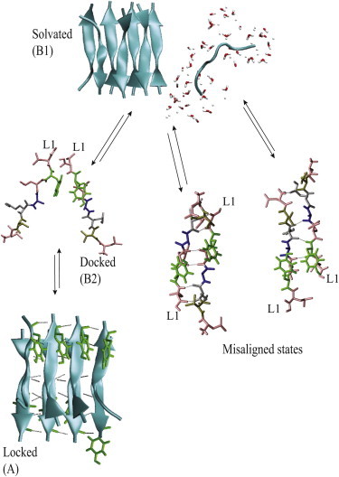
Addition of a solvated peptide monomer to the fibril. A fully solvated peptide can attach to the fibril in various ways. Proper docking ensures correct alignment of the peptide monomer with the fibril. Otherwise, various misaligned states can be encountered.

To avoid these metastable traps, we will focus on the transition between the docked and locked states, which is generally thought to be the rate-limiting step (11,16). To do so, we redefine stable state B to include, in addition to the solvated state, the docked state. The system is now considered to have reached the final state $\text{B}2$ if the distances of the core native contacts ($d\text{E}3\text{E}$, $d\text{A}4\text{A}$, and $d\text{L}5\text{L}$) are >1.0 nm. This new definition of state $\text{B}2$ is more flexible, as it includes both docked and fully solvated states. Note that although this definition allows for paths that connect the locked state with another metastable state than the docked state, we did not observe such paths in the second set of TPS simulations. The new stable-state definitions are summarized in Table 2. Again, we stress that the labels A and $\text{B}2$ are entirely interchangable, as TPS employs time-reversible dynamics and thus samples the reversible process $\text{A}\rightleftharpoons \text{B}2$.

Starting from the initial path selected from the SMD simulations, 10 independent TPS simulations were performed. The acceptance ratio was 32%, resulting in a path ensemble of 380 paths. As we are using the one-way shooting algorithm, the decorrelation time is quite large (45), and we estimated from the sampling trees that in total 25 paths are decorrelated by having lost all memory of their previous decorrelated path. The distribution of the path lengths is shown in Fig. 5. Note the Poissonian shape, characteristic of a stochastic process (29). The average path length in the ensemble is 906 ps and the aggregate simulation time is 0.75 μs. The results indicate that the observed path ensemble is an equilibrium path ensemble for which the dependence on the initial path is small.

Figure 5.

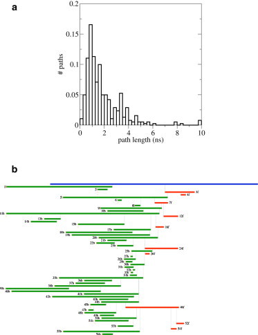
(a) Normalized distribution of path lengths of the accepted paths. (b) Example of a sampling tree. Accepted forward shooting paths are shown going to the right, accepted backward paths to the left.

Inspection of the sampling trees of the TPS simulations (for example, the one shown in Fig. 5) shows that backward accepted paths to the locked state are much more frequent than forward accepted paths to the docked state (approximately five backward paths are accepted for every forward accepted path). This behavior is likely to be a consequence of using the one-way shooting algorithm in a rough free-energy landscape in which the transition state is located close to the final state and/or the presence of relatively long-lived metastable states between the initial state and the transition state.

The 25 decorrelated paths follow roughly two major routes. In Fig. 6, two typical trajectories are shown in the plane of two of the order parameters used to define the stable states. All trajectories start in a state with all backbone hydrogen bonds formed. In this state, a hydrogen bond is present between the Ala backbone oxygen of SH1P1 and the Glu side chain of SH2P1, and the Glu side chain of SH1P1 is oriented toward SH2P1. All trajectories end in a conformation where SH1P1 and SH1P2 are interacting through L7 only. In this state, the hydrogen-bond distance $dYoLn$ is usually <0.35 nm, indicative of a formed hydrogen bond.

Figure 6.

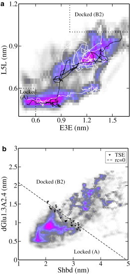
Path densities and TSE. (a) Path densities and representative paths plotted in the dE3E–dL5L plane indicate that there are two routes connecting the docked and the locked states. Stable states are indicated by dotted lines. The white path corresponds to route a in Fig. 7, and the black path corresponds to route b. (b) Path densities and the predicted TSE (triangles) for RC2 projected on the Shbd–dGlu1.3A2.4 plane. The dashed line shows the predicted dividing surface r = 0 for RC2.

The path density visualizes the path ensemble by quantifying the number of paths passing through a certain point in order-parameter space. The path density in the dE3E–dL5L plane indicates that there are two major routes connecting these two states: one in which a large increase in $d\text{E}3\text{E}$ is followed by an increase in $d\text{L}5\text{L}$ (Fig. 6 a, white path) and the other in which, upon a smaller increase in $d\text{E}3\text{E}$, $d\text{L}5\text{L}$ is first to increase followed by a simultaneous increase in both order parameters (Fig. 6 a, black path). This second route corresponds to Fig. 7, route a, where the Glu side chain from SH1P1 remains oriented toward SH2P1 while hydrogen bonds between SH1P1 and SH1P2 are broken. Once the side chain changes orientation, the peptide is in the docked state. Alternatively, following Fig. 7, route b, the Glu side chain changes orientation before breaking of the core hydrogen bonds. Regardless of the route followed, the trajectories spend a relatively long time (up to ∼150 ps) sampling a region close to the locked state and another region close to the docked state, suggesting that these regions may be additional metastable intermediate states.

Figure 7.

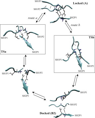
Snapshots from two decorrelated paths following different routes from state A to $\text{B}2$. For clarity, only the Glu and Ala side chains are shown in licorice representation. Route a (left) shows that the Glu side chain from SH1P1 remains oriented toward SH2P1 while hydrogen bonds between SH1P1 and SH1P2 are broken (TSa). In the next step, the Glu side chain becomes fully solvated followed by transition to state B. The other possibility (route b) is for the Glu side chain to change orientation before breaking of the core hydrogen bonds (TSb). Structures for TSa and TSb are taken from the predicted TSE (see Table 3 and Fig. 6).

Reaction-coordinate analysis and the transition-state ensemble

Likelihood maximization analysis was conducted on the set of 555 backward shooting points. For this set of shooting points the minimum increase in log likelihood by adding more parameters to the reaction coordinate is $\delta L_{\text{min}}=3.159$. We tested all possible linear combinations of one, two, and three order parameters for this set. The optimal reaction coordinates are shown in Table 3. Note that using a linear combination of multiple order parameters to describe the reaction coordinate does not prove significant according to the Bayesian information criterion $\left(\delta L<3.159\right)$. However, the combination of order parameters making up RC2 does give a better understanding of the mechanism under study. Moreover, both Shbd and $d\text{Glu}1.3\text{A}2.4$ score well in LM analysis for one order parameter (with lnL = −350.2 and lnL = −350.7, respectively). When a combination of three order parameters is used to describe the reaction coordinate (RC3), the radius of gyration of the locking peptide, $Rg1$, is added to the previously identified order parameters Shbd and $d\text{Glu}1.3\text{A}2.4$. As hydrogen bonds are formed between the peptide and the fibril, the peptide will extend and increase its radius of gyration. Still, adding a third component to the reaction coordinate does not improve the likelihood significantly.

Table 3.

Reaction coordinates predicted by likelihood maximization analysis

n	lnL	Reaction coordinate
1	−347.4	1.924 − 2.014 dE3E
2	−345.1	1.912 − 0.387 Shbd − 0.7332 dGlu1.3A2.4
3	−343.2	−1.037 − 0.402 Shbd + 4.266 Rg1 − 0.672 dGlu1.3A2.4

From the shooting point ensemble, a prediction of the transition-state ensemble (TSE) can be extracted by locating structures with $r\approx 0$ (within the interval $-0.05<r<0.05$) for the reaction coordinates identified. Although the predicted TSEs should in principle be tested by committor analysis, this is computationally expensive and we did not perform such tests. Fig. 6 b depicts the predicted TSE together with the path densities in the plane of Shbd and $d\text{Glu}1.3\text{A}2.4$, order parameters identified in RC2. The predicted TSE for both RC1 and RC2 contains structures similar to those presented in Fig. 7. (TSa and TSb). Viewed from the solvation perspective, all structures have lost the native contacts of the N-terminal three residues (L1, V2, and E3), and the hydrogen bond between the Glu side chain of SH2P1 and the Ala backbone of SH1P1 is broken. The TSE extracted for RC2 seems to indicate two different transition-state regions. As discussed above, the main difference between these two subensembles is in the orientation of the Glu side chain of SH1P1. This side chain can remain oriented toward the lower sheet while the backbone hydrogens between A4 and L5 of SH1P1 and SH1P2 are broken. Otherwise, the Glu side chain can be solvated, in which case the backbone hydrogen bonds are still intact. We finally note that the RC analysis as performed here could be improved by allowing for nonlinear coordinates using the complete path ensemble (49).

Conclusions

The TPS simulations suggest the following mechanism for the incorporation of a peptide monomer to a fibril of LVEALYL (see Figs. 4 and 7). In the first step, the peptide docks by forming contacts between the C-terminal Leu and Tyr and the corresponding residues in the fibril. After docking, the peptide has to change conformation to commensurate the fibril template. To do so, two routes can be followed (Figs. 6 and 7). In one route, the locking peptide first forms most of its backbone hydrogen bonds, followed by reorientation of the Glu side chain of the locking peptide toward the interface between the β-sheets. This reorientation is followed by the formation of the final backbone hydrogen bond. Alternatively, the orientation of the Glu side chain can change before the formation of the backbone hydrogen bonds.

Our results indicate that the docked state, where the C-terminal leucine contacts are formed, is important for proper alignment of the locking peptide with the fibril. Locking involves hydrogen-bond formation between the protonated glutamate side chain of a peptide in the opposite sheet to the alanine backbone of the locking peptide. The reaction coordinate identified through likelihood-maximization analysis indicates that the orientation of the Glu side chain of the locking peptide toward the opposite sheet is an important step.

We have shown that TPS can be used to gain new insight into amyloid fibril growth of the LVEALYL heptapeptide. Up to now, insights into the dock-lock mechanism have come mainly from much more computationally expensive straightforward MD simulations (12,14).

Our initial TPS simulations revealed the docked state as an intermediate state, even though the SMD simulations did not identify it as such. We expect that there is large hysteresis when starting SMD simulations from the fully solvated state or the locked state. In addition, the occurrence of metastable misaligned states in this TPS simulation suggests that docking is an important step in the proper alignment of the peptide with the fibril template. This observation probably also holds for most other short, amyloid-forming peptides. The locking process is likely to be more sequence-specific than the docking process, as more contacts between the peptide and the fibril have to be formed. It would be interesting to compare various amyloid systems to gain a more general insight into the essential interactions in the locking process.

The work described assumes a growth of a perfectly ordered fibril. This is an idealization, and in general it is quite possible that the growing fibril is partly disordered.

Our predictions of the mechanism could be tested experimentally, e.g., by point mutation (phi analysis) of the glutamic acid residue, or by spectroscopic methods such as infrared and 2D infrared spectroscopy that specifically target the Glu and Tyr residues.

Future simulation work on this system could focus on the rate constants for the dock-lock transition and the free-energy landscape. Also, the evaluation of nonlinear reaction coordinates (49) could be of interest.

References

- 1.Dobson C.M. Protein folding and misfolding. Nature. 2003;426:884–890. doi: 10.1038/nature02261. [DOI] [PubMed] [Google Scholar]
- 2.Selkoe D.J. Folding proteins in fatal ways. Nature. 2003;426:900–904. doi: 10.1038/nature02264. [DOI] [PubMed] [Google Scholar]
- 3.Chiti F., Dobson C.M. Protein misfolding, functional amyloid, and human disease. Annu. Rev. Biochem. 2006;75:333–366. doi: 10.1146/annurev.biochem.75.101304.123901. [DOI] [PubMed] [Google Scholar]
- 4.Badtke M.P., Hammer N.D., Chapman M.R. Functional amyloids signal their arrival. Sci. Signal. 2009;2:pe43. doi: 10.1126/scisignal.280pe43. [DOI] [PMC free article] [PubMed] [Google Scholar]
- 5.Greenwald J., Riek R. Biology of amyloid: structure, function, and regulation. Structure. 2010;18:1244–1260. doi: 10.1016/j.str.2010.08.009. [DOI] [PubMed] [Google Scholar]
- 6.Cherny I., Gazit E. Amyloids: not only pathological agents but also ordered nanomaterials. Angew. Chem. Int. Ed. Engl. 2008;47:4062–4069. doi: 10.1002/anie.200703133. [DOI] [PubMed] [Google Scholar]
- 7.Channon K., MacPhee C.E. Possibilities for smart materials exploiting the self-assembly of polypeptide fibrils. Soft Matter. 2008;4:647–652. doi: 10.1039/b713013a. [DOI] [PubMed] [Google Scholar]
- 8.Knowles T.P.J., White D.A., Weitz D.A. Observation of spatial propagation of amyloid assembly from single nuclei. Proc. Natl. Acad. Sci. USA. 2011;108:14746–14751. doi: 10.1073/pnas.1105555108. [DOI] [PMC free article] [PubMed] [Google Scholar]
- 9.Collins S.R., Douglass A., Weissman J.S. Mechanism of prion propagation: amyloid growth occurs by monomer addition. PLoS Biol. 2004;2:e321. doi: 10.1371/journal.pbio.0020321. [DOI] [PMC free article] [PubMed] [Google Scholar]
- 10.Cannon M.J., Williams A.D., Myszka D.G. Kinetic analysis of β-amyloid fibril elongation. Anal. Biochem. 2004;328:67–75. doi: 10.1016/j.ab.2004.01.014. [DOI] [PubMed] [Google Scholar]
- 11.Esler W.P., Stimson E.R., Maggio J.E. Alzheimer’s disease amyloid propagation by a template-dependent dock-lock mechanism. Biochemistry. 2000;39:6288–6295. doi: 10.1021/bi992933h. [DOI] [PubMed] [Google Scholar]
- 12.Nguyen P.H., Li M.S., Thirumalai D. Monomer adds to preformed structured oligomers of Aβ-peptides by a two-stage dock-lock mechanism. Proc. Natl. Acad. Sci. USA. 2007;104:111–116. doi: 10.1073/pnas.0607440104. [DOI] [PMC free article] [PubMed] [Google Scholar]
- 13.O’Brien E.P., Okamoto Y., Thirumalai D. Thermodynamic perspective on the dock-lock growth mechanism of amyloid fibrils. J. Phys. Chem. B. 2009;113:14421–14430. doi: 10.1021/jp9050098. [DOI] [PMC free article] [PubMed] [Google Scholar]
- 14.Reddy G., Straub J.E., Thirumalai D. Dynamics of locking of peptides onto growing amyloid fibrils. Proc. Natl. Acad. Sci. USA. 2009;106:11948–11953. doi: 10.1073/pnas.0902473106. [DOI] [PMC free article] [PubMed] [Google Scholar]
- 15.Sawaya M.R., Sambashivan S., Eisenberg D. Atomic structures of amyloid cross-β spines reveal varied steric zippers. Nature. 2007;447:453–457. doi: 10.1038/nature05695. [DOI] [PubMed] [Google Scholar]
- 16.Massi F., Straub J.E. Energy landscape theory for Alzheimer’s amyloid β-peptide fibril elongation. Proteins. 2001;42:217–229. doi: 10.1002/1097-0134(20010201)42:2<217::aid-prot90>3.0.co;2-n. [DOI] [PubMed] [Google Scholar]
- 17.Brange J., Andersen L., Rasmussen E. Toward understanding insulin fibrillation. J. Pharm. Sci. 1997;86:517–525. doi: 10.1021/js960297s. [DOI] [PubMed] [Google Scholar]
- 18.Ahmad A., Uversky V.N., Fink A.L. Early events in the fibrillation of monomeric insulin. J. Biol. Chem. 2005;280:42669–42675. doi: 10.1074/jbc.M504298200. [DOI] [PubMed] [Google Scholar]
- 19.Nielsen L., Khurana R., Fink A.L. Effect of environmental factors on the kinetics of insulin fibril formation: elucidation of the molecular mechanism. Biochemistry. 2001;40:6036–6046. doi: 10.1021/bi002555c. [DOI] [PubMed] [Google Scholar]
- 20.Hong D.-P., Ahmad A., Fink A.L. Fibrillation of human insulin A and B chains. Biochemistry. 2006;45:9342–9353. doi: 10.1021/bi0604936. [DOI] [PubMed] [Google Scholar]
- 21.Dische F.E., Wernstedt C., Watkins P.J. Insulin as an amyloid-fibril protein at sites of repeated insulin injections in a diabetic patient. Diabetologia. 1988;31:158–161. doi: 10.1007/BF00276849. [DOI] [PubMed] [Google Scholar]
- 22.Störkel S., Schneider H.M., Kashiwagi S. Iatrogenic, insulin-dependent, local amyloidosis. Lab. Invest. 1983;48:108–111. [PubMed] [Google Scholar]
- 23.Ivanova M.I., Sievers S.A., Eisenberg D. Molecular basis for insulin fibril assembly. Proc. Natl. Acad. Sci. USA. 2009;106:18990–18995. doi: 10.1073/pnas.0910080106. [DOI] [PMC free article] [PubMed] [Google Scholar]
- 24.Park S., Khalili-Araghi F., Schulten K. Free energy calculation from steered molecular dynmics simulations using Jarzynski’s equality. J. Chem. Phys. 2003;119:3559–3566. [Google Scholar]
- 25.Torrie G.M., Valleau J.P. Nonphysical sampling in Monte Carlo free-energy estimation: umbrella sampling. J. Comput. Phys. 1977;23:141–151. [Google Scholar]
- 26.Laio A., Parrinello M. Escaping free-energy minima. Proc. Natl. Acad. Sci. USA. 2002;99:12562–12566. doi: 10.1073/pnas.202427399. [DOI] [PMC free article] [PubMed] [Google Scholar]
- 27.Sugita Y., Okamoto Y. Replica-exchange molecular dynamics method for protein folding. Chem. Phys. Lett. 1999;314:141–151. [Google Scholar]
- 28.Buchete N.V., Hummer G. Peptide folding kinetics from replica exchange molecular dynamics. Phys. Rev. E Stat. Nonlin. Soft Matter Phys. 2008;77:030902. doi: 10.1103/PhysRevE.77.030902. [DOI] [PubMed] [Google Scholar]
- 29.Dellago C., Bolhuis P.G., Geissler P.L. Transition path sampling. Adv. Chem. Phys. 2002;123:1–78. doi: 10.1146/annurev.physchem.53.082301.113146. [DOI] [PubMed] [Google Scholar]
- 30.Peters B., Trout B.L. Obtaining reaction coordinates by likelihood maximization. J. Chem. Phys. 2006;125:054108. doi: 10.1063/1.2234477. [DOI] [PubMed] [Google Scholar]
- 31.Peters B., Beckham G.T., Trout B.L. Extensions to the likelihood maximization approach for finding reaction coordinates. J. Chem. Phys. 2007;127:034109. doi: 10.1063/1.2748396. [DOI] [PubMed] [Google Scholar]
- 32.Oostenbrink C., Villa A., van Gunsteren W.F. A biomolecular force field based on the free enthalpy of hydration and solvation: the GROMOS force-field parameter sets 53A5 and 53A6. J. Comput. Chem. 2004;25:1656–1676. doi: 10.1002/jcc.20090. [DOI] [PubMed] [Google Scholar]
- 33.Berendsen H.J.C., Postma J.P.M., van Gunsteren W.F., Hermans J. Interaction models for water in relation to protein hydration. In: Pullman B., editor. Interaction Forces. Reidel, Dordrecht; The Netherlands: 1981. pp. 331–342. [Google Scholar]
- 34.Todorova N., Legge F.S., Yarovsky I. Systematic comparison of empirical forcefields for molecular dynamic simulation of insulin. J. Phys. Chem. B. 2008;112:11137–11146. doi: 10.1021/jp076825d. [DOI] [PubMed] [Google Scholar]
- 35.Hess B., Kutzner C., Lindahl E. GROMACS 4: algorithms for highly efficient, load-balanced and scalable molecular dynamics. J. Chem. Theory Comput. 2008;4:435–447. doi: 10.1021/ct700301q. [DOI] [PubMed] [Google Scholar]
- 36.Hess B., Bekker H., Fraaije J.G.E.M. LINCS: a linear constraint solver for molecular simulations. J. Comput. Chem. 1997;18:1463–1472. [Google Scholar]
- 37.Miyamoto S., Kollman P.A. SETTLE: an analytical version of the SHAKE and RATTLE algorithms for rigid water molecules. J. Comput. Chem. 2001;13:952–962. [Google Scholar]
- 38.Bussi G., Donadio D., Parrinello M. Canonical sampling through velocity rescaling. J. Chem. Phys. 2007;126:014101. doi: 10.1063/1.2408420. [DOI] [PubMed] [Google Scholar]
- 39.Parrinello M., Rahman A. Polymorphic transitions in single crystals: a new molecular dynamics method. J. Appl. Phys. 1981;52:7182–7190. [Google Scholar]
- 40.Park S., Schulten K. Calculating potentials of mean force from steered molecular dynamics simulations. J. Chem. Phys. 2004;120:5946–5961. doi: 10.1063/1.1651473. [DOI] [PubMed] [Google Scholar]
- 41.Jarzynski C. Nonequilibrium equality for free energy differences. Phys. Rev. Lett. 1997;78:2690–2693. [Google Scholar]
- 42.Juraszek J., Bolhuis P.G. Sampling the multiple folding mechanisms of Trp-cage in explicit solvent. Proc. Natl. Acad. Sci. USA. 2006;103:15859–15864. doi: 10.1073/pnas.0606692103. [DOI] [PMC free article] [PubMed] [Google Scholar]
- 43.Vreede J., Juraszek J., Bolhuis P.G. Predicting the reaction coordinates of millisecond light-induced conformational changes in photoactive yellow protein. Proc. Natl. Acad. Sci. USA. 2010;107:2397–2402. doi: 10.1073/pnas.0908754107. [DOI] [PMC free article] [PubMed] [Google Scholar]
- 44.Bolhuis P.G. Transition path sampling on diffusive barriers. J. Phys. Condens. Matter. 2003;15:S113–S120. [Google Scholar]
- 45.Bolhuis P.G., Dellago C. Trajectory based rare event simulations. Rev. Comput. Chem. 2010;27:111–210. [Google Scholar]
- 46.Vanden-Eijnden E. Towards a theory of transition paths. J. Stat. Phys. 2006;123:503–523. [Google Scholar]
- 47.Metzner P., Schütte C., Vanden-Eijnden E. Illustration of transition path theory on a collection of simple examples. J. Chem. Phys. 2006;125:084110. doi: 10.1063/1.2335447. [DOI] [PubMed] [Google Scholar]
- 48.Wolf M.G., Jongejan J.A., de Leeuw S.W. Quantitative assessment of amyloid fibril growth of short peptides from simulations: calculating association constants to dissect side chain importance. J. Am. Chem. Soc. 2008;130:13493–13498. doi: 10.1021/ja806606y. [DOI] [PubMed] [Google Scholar]
- 49.Lechner W., Rogal J., Bolhuis P.G. Nonlinear reaction coordinate analysis in the reweighted path ensemble. J. Chem. Phys. 2010;133:174110. doi: 10.1063/1.3491818. [DOI] [PubMed] [Google Scholar]
- 50.Humphrey W., Dalke A., Schulten K. VMD: visual molecular dynamics. J. Mol. Graph. 1996;14:33–38. doi: 10.1016/0263-7855(96)00018-5. 27–28. [DOI] [PubMed] [Google Scholar]