A brief survey of symmetry in mathematics

Abstract

This paper presents a brief survey of the idea of symmetry in mathematics, as exemplified by some particular developments in algebra, differential equations, topology, and number theory.

At this conference on Symmetries Throughout the Sciences, I thought that it might be of interest to survey briefly how the idea of symmetry has developed in its native habitat—mathematics.

Section 1

Every congruence of two triangles in the Euclidean plane gives a symmetry of the plane. But millenia passed before mathematicians began to consider the totality of symmetries G of the plane. Once that is done, one sees that there is an algebraic operation on G combining two elements to get a third, namely the composition g·h, which sends any point x to g(h(x)). If one extracts the notion of group from this context, a group G is a set with a binary operation (g₁, g₂) → g₁·g₂, which is associative: (g₁·g₂)·g₃ = g₁·(g₂·g₃), has an identity element 1 such that g·1 = 1·g for all g in G, and each g in G has an inverse g⁻¹ such that g⁻¹·g = 1 = g·g⁻¹. Towards the end of the 18^th century, this idea was used by J. L. Lagrange, A. T. Vandermonde, and P. Ruffini. One of the great advances in mathematics was the exploitation of this new notion by E. Galois (1811–1832) in an algebraic context.

Let f(x) = xⁿ + a₁xⁿ⁻¹ + … + a_n be a polynomial with coefficients in the field ℚ of rational numbers {m/n; m, n ∈ ℤ, the ring of integers}. Then with the use of complex numbers, f(x) = ∏_i=1ⁿ (x − θ_i) factors into linear factors, θ_i being the roots of f(x).

Galois considered the group of all permutations of the roots θ₁, … , θ_n, which respect addition and multiplication of all expressions formed by them together with rational numbers in the field they generate.

This simple idea has had far reaching applications. To give a rudimentary example, consider the field generated by the roots of

Let ζ = cos 2π/8 + i sin 2π/8 = /2 + i /2. Then the zeros of x⁸ − 1 are 1, ζ, … , ζ⁷, and ζ satisfies x⁴ + 1 = 0. The group G of automorphisms of the field ℚ(ζ) consists of the four automorphisms

where gcd(n, 8) = 1, i.e., n = 1, 3, 5, 7.

Each element of the Galois group G other than σ₁ has order 2; since

Then {σ₁, σ_n} forms a subgroup of two elements ≈ ℤ/2ℤ, n = 3, 5, 7

G has three subgroups different from σ₁.

In the field ℚ(ζ)(= ℚ[i, ]),

That is, to each subgroup H of G there corresponds the unique subfield of ℚ(ζ) whose elements it fixes, and conversely each subfield F of ℚ(ζ) arises in this way. Finally, the number of elements in G = dim(ℚ(ζ), the dimension of ℚ(ζ) as a vector space with scalars ℚ.

These relations between a field generated by all the roots of a polynomial in ℚ[x] and its Galois group hold generally.

Galois introduced the notion of normal subgroup (he called it “propre”), proved that an irreducible polynomial of degree 5 or greater cannot be expressed by radicals, and exhibited such irreducible polynomials. N. Abel (1802–1829) proved a similar result but only for “general polynomials” with indeterminate coefficients.

As an even easier application, one could settle the long-standing geometric conjectures about the impossibility of angle trisection and cube doubling via compass and ruler construction.

The interest in crystallography led to the study of a class of infinite groups. M. L. Frankenheimer in 1842 classified all the crystallographic lattices in ℝ³; these are groups Γ, which contain a subgroup T of translations in three independent directions in 3-space, and moreover the set of cosets {xT; x ∈ Γ}, which is denoted Γ/T, is a finite set. Indeed, if we take T to be the subgroup of all translations in Γ, then xTx⁻¹ = T and thus Γ/T is a finite group. In 1850, Auguste Bravais reworked Frankenheimer’s results more rigorously, discovering that there were only 14 types of crystallographic groups in ℝ³, correcting Frankenheimer’s claim of 15. These are known as Bravais lattices.

We’ll come back to lattices later.

Section 2

Let us turn now to “finite continuous” groups—these contain an infinity of elements parametrized by a finite number of parameters. The first major achievement was by the Norwegian mathematician, Sophus M. Lie (1842–1899), who in 1873–1874 associated to each such group its algebra of infinitesimal generators. By definition, an infinitesimal generator in local coordinates (x₁, … , x_n) is an operator

which describes how the smooth function f changes at the points x in the direction (ξ¹(x), … , ξⁿ(x)).

Geometrically, X defines a vector field, which we can think of as the velocity field of the flow dxⁱ/dt = ξⁱ(x)(i = 1, … , n). The resulting flow after time t results in the “finite transformation” denoted exp t X, which moves each point to its downstream position after time t. This general notion agrees with the usual exponential:

If A is any n × n matrix and ξ(x) = Ax for x ∈ ℝⁿ, then exp t A = e^tA.

Lie’s earliest interest was in getting quadratures for differential equations from symmetries. Later, he studied the group structures. If G is a “finite continuous” group, with u, v, w in G and w = u·v, then the group multiplication law is specified by r functions of 2r variables, r = dimG. The big idea of Lie was that group multiplication can be determined by merely r³ numbers in the following way.

A finite continuous transformation group G on a space M is specified by:

(i) smooth manifolds G and M,

(ii) a multiplication G × G → G:(g₁, g₂) → g₁g₂,

(iii) an action G × M → M:(g, m) → g(m) of G on M such that (g₁g₂)(m) = g₁(g₂(m)).

Let c(t) be any smooth curve in G with c(0) = 1. Then m → dc(t)(m)/dt_|t=0 is a vector field on M. Let 𝔊 denote the totality of such vector fields. In the special case where G acts on itself by left multiplication, we call 𝔊 the Lie algebra of G; it is often denoted Lie(G).

Properties:

1.  X, Y ∈ 𝔊 ⇒ X + Y ∈ 𝔊, aX ∈ 𝔊, for all a ∈ ℝ.

2.  X, Y ∈ 𝔊 ⇒ [X, Y] ∈ 𝔊 (where for any function f on M, [X, Y]f = XYf − YXf).

3.  [X[Y, Z]] + [Z, [X, Y]] + [Y[Z, X]] = 0.

4.  dim 𝔊 ≤ dim G, with equality if g(m) = m for all m ∈ M implies g = 1.

Let {X₁, … , X_r} be a base for Lie(G). Then [X_i, X_j] = Σ_k=1^r c_i,j^k X_k, c_i,j^k ∈ ℝ.

The r³ constants c_i,j^k are called Lie’s constants of structure.

Lie introduced the notion of a simple group G—one having no normal subgroup of positive dimension ≠ G. He listed four “great” classes of simple groups of rank n:

These are the matrix groups that preserve det, x₁² + … + x_2n+1², a skew-symmetric bilinear form in x₁, … , x_2n, and x₁² + … + x_2n², respectively. He had in mind the group with complex entries. The rank n refers to the dimension of any maximal diagonalizable subgroup of G—all such being conjugate under an inner automorphism (Fig. 1).

Figure 1.

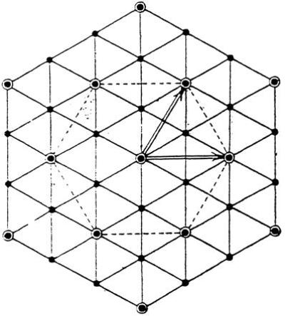
Unitary group SU(3) = simply connected compact real form of SL(3).

W. Killing in 1888–1889, classified all simple Lie algebras (over ℂ) of rank n (1, 2). His results needed a slight correction, which Cartan did in this 1896 thesis. Hermann Weyl put Cartan’s classification into a more geometric form, which permits us to give a remarkably vivid picture of the classification.

To each simple Lie group, there corresponds a unique simply connected simple Lie group G (i.e., any circle in G can be deformed to a point.) Each simple Lie group G over ℂ has a maximal compact subgroup G_K unique up to conjugacy. Lie (G_K) is a real Lie algebra and Lie(G) = Lie(G_K) ⊗ ℂ; that is, the complex Lie algebra Lie(G) consists of complex Lie combinations of elements of Lie(G_K).

Choose T, a maximal diagonalizable subgroup of G_K (all such T are conjugate in G_K). G acts on itself by inner automorphisms. This action induces a linear action on the Lie algebra 𝔊 called the adjoint representation.

Decompose 𝔊 = ⊕𝔊_α into spaces of common eigenvectors for Ad T, i.e., Ad(t)X_α = α(t)X_α for all X_α ∈ 𝔊_α, t ∈ T.

Let L = Ker exp: Lie(T) → T; i.e., x ∈ L ↔ x ∈ Lie(T) and expX = 1. Then L is a lattice in the sense of crystallography.

Let N(T) = {g ∈ G; gTg⁻¹ = T}. Then N(T) acts on Lie(T) and stabilizes L. Moreover, W = N(T)/T acts faithfully on L.

Γ = W × L (semi-direct product) is a crystallographic group; we call it “highly symmetric”, by which we mean that Γ is generated by reflections in the n + 1 faces of an n-dimensional simplex (Fig. 1).

The classification of simple Lie groups can be formulated as: The correspondence

is a 1 − 1 correspondence. Indeed all the information about the algebraic and geometric structure of G can be deduced from the crystal structure (1).

The early interest of S. Lie in applications of infinitesimal symmetries to differential equations has borne fruit. Well known to physicists is the theorem of E. Noether (1918) that to each infinitesimal symmetry there corresponds a conservation law (3).

Starting with a paper of Date et al. (4), a remarkable link was discovered between representation theory of affine Lie algebras and the Korteweg–deVries nonlinear partial differential equations. Starting in 1978, it has been realized that complete integrability is related to Lie algebra theory and that both Korteweg–deVries equations and Toda systems can be viewed as Hamiltonian systems in the co-adjoint orbit of a suitable Lie algebra (2, 5, 6).

Section 3

The most important application of groups to topology lies in the construction via groups of special space prototypes in terms of which all spaces can be analyzed. The construction is via quotient spaces whose points are cosets of a group.

We consider in this section quotients of compact groups. In the next section, we consider quotients of noncompact groups by discrete subgroups.

A fiber bundle (E, B, F, π, G) with total space E, base B, fiber F, projection π:E → B, and group G is specified by a collection of open sets {V_i} covering B and by homeomorphisms for each index i:

satisfying

1

where g_ji(v) ∈ G and is continuous in v ∈ V_i ∩ V_j.

For example, a möbius strip is the total space of a fiber bundle over the circle S¹, with fiber the unit interval I = [0, 1] and the group G = ℤ/(2) acting by flipping I.

If in Eq. 1 we replace the fiber F by the group G acting on itself by left multiplication, we obtain the “principal” G-bundle associated to (E, B, F, π, G), which we denote (P, B, G, π). Since left and right multiplication in any group commute, the action of G on P by right multiplication can be defined unambiguously. A principal G-bundle (P_G, B_G, G, π_G) is called n-universal, if and only if π_k(P_G) = 0, 0 ≤ k < n; i.e., any map of the k-sphere S^k to P_G can be deformed to a point for all k < n. Its basic property is: For any principal G-bundle (P, B, G, π) with dimB ≤ n, there is a G-bundle map f:(P, B, G, π) → (P_G, B_G, G, π_G) (i.e., f is continuous and respects fibers and hence defines a map f:B → B_G) and therefore the bundle (P, B, G, π) is equivalent to the pull-back bundle, defined as

We can take as N-universal U(q) bundle the principal bundle (P_G, B_G, U(q), π_G) with

Clearly dim_ℂ Gr(q, N, ℂ) = qN.

Fix ℂ^i+N−i in ℂ^q+N. Let

𝒵_i is called a Schubert cycle; dim_ℝ 𝒵_i = 2(qN − i). Intersections of 𝒵_i with cycles of dim 2_i defines a linear function on the homology group H_2i(Gr(q, N, ℂ), ℤ); hence, an element c_i the cohomology group H²ⁱ(Gr(q, N, ℤ)).

The i^th Chern class of principal bundle (P, B, G, π) is defined as the element in H²ⁱ(B, ℤ) given by

where N is taken ≥ dim B.

These topological invariants can be expressed in terms of the curvature of the bundle

Example. (P, B, G, π) with G = GL(q, ℂ)

φ = connection on bundle = 1-form, values in Lie(G),

Φ = curvature = dφ − 1/2 [φ, φ] is a Lie(G) − valued 2 − form on p

det(λI_q − 1/(2π) X) = λ^q + F₁(X)λ^q−1 + … + F_q(X), x ∈ Lie(G).

Then F_i(Φ) = c_i(P, B, G, π) ∈ H²ⁱ(B, ℤ) (7).

The foregoing ideas are exploited in Yang–Mills theories.

Section 4. Discrete Groups

By a lattice Γ in a Lie group G, we mean a subgroup which is

(i) discrete (i.e., no accumulation points),

(ii) G/Γ has finite Haar measure.

Example. SL(n, ℤ) is a lattice in SL(n, ℝ).

Borel–Harish–Chandra Theorem (1961). G(ℤ) is a lattice in G(ℝ) for any algebraic group defined over ℚ with no homomorphisms to scalars defined over ℚ (8).

Such lattices and closely related ones are called arithmetic.

A near converse to the foregoing theorem is the

Margulis Theorem (1974). A lattice in a semi-simple group of ℝ-rank > 1 and with no ℝ-rank 1 factors is arithmetic (9).

Margulis’ result came from a strengthening of the following rigidity theorem.

Theorem (Mostow, 1972). Let G, G′ be semi-simple Lie groups having no compact factors and no centers. Let Γ, Γ′ be lattices in G, G′, respectively. Assume G/Γ and G′/Γ′ are compact, and θ:Γ → Γ′ is an isomorphism. Then θ extends to an analytic isomorphism G → G′, except in the case that G = SL(2, ℝ)/± 1.

Underlying the proof of this rigidity theorem is the study of the space of double cosets K/G/Γ associated to the pair (G, Γ), where K is a maximal compact subgroup (10). The space K/G is a symmetric Riemannian space; at each of its points, the map reversing the direction of geodesics gives an isometry of the space [Example: hyperbolic n-space = SO(n)/SO_o(n, 1)]. The space K/G/Γ for (G, K) as above and Γ a discrete subgroup is a locally symmetric space.

This rigidity result is false for SL(2, R)/± 1, as is well-known from the theory of one complex variable.

Margulis’ strengthening consisted in replacing the hypothesis on Γ′ by a weaker one, permitting θ to be a homomorphism, and implementing the boundary map strategy used in proving rigidity, but replacing the geometric arguments in Mostow’s proof by measure theoretic arguments based on the “multiplicative ergodic theorem.”

The applications of the rigidity theorem that have been made by W. Thurston to the study of three-dimensional manifolds depend on the 1968 version that was proved for SO(1, n) using the theory of quasi-conformal mappings in n-space (11). (The first version assumes that G/Γ is compact; subsequently, the general strategy was extended by Gopal Prasad to the case of arbitrary lattices in SO(1, n), (n > 1)) (12).

As a consequence of this rigidity theorem, the metric invariants of n-dimensional manifolds (n > 2) having finite volume hyperbolic structure are topological invariants!

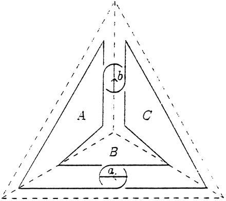
Thurston’s central conjecture is that 3-manifolds can be decomposed canonically into pieces each having geometric structure K/G/Γ, a space of double cosets of a group (13). In some of the most important cases, the geometric structure is finite volume hyperbolic. For example, the complement of a figure-eight knot in S³ (Figs. 2, 3, 4, 5), or that obtained by (p, q) Dehn surgery has finite volume hyperbolic structure if |p| > 4 or |q| > 1. The proof is based on remarkable geometry-guided computations (14).

Figure 2.

The figure-eight knot.

Figure 3.

A regular ideal tetrahedron in B³.

Figure 4.

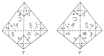
The gluing pattern figure-eight knot complement.

Figure 5.

The figure-eight knot draped over the tetrahedron T.

Another line of investigation in topology has been directed at topological characterization of spaces, which admit negatively curved metrics resembling those on negatively curved locally symmetric spaces (15).

Section 5. Number Theory

We conclude with a bare bones statement of the ongoing Langlands program (16, 17).

The locally compact adele ring 𝔸 of ℚ is defined as

the restricted direct product of the field ℝ and the p-adic completions ℚ_p for all primes p. Then ℚ embeds diagonally in 𝔸 and its image is discrete. Consider G = GL(n), G(𝔸) = GL(n, 𝔸), and G(ℚ) = GL(n, ℚ), which is discrete in G(𝔸). We define the regular representation R of G(𝔸) on L² (G(ℚ)/G(𝔸)) via R(g)f(x) = f(xg) for x, g ∈ G. A representation π of G(𝔸) is called automorphic if and only if π is irreducible, unitary, and occurs in the decomposition of R or from an analytic continuation of such.

The decomposition alluded to here owes much to profound work of Harish-Chandra and, later, Langlands (18, 19). Then π decomposes as a tensor product

with each π_p an irreducible unitary representation of G(ℚ_p). For all p ∉ some finite set S_π, π_p contains a vector fixed by G(ℤ_p). By the representation theory of ℚ_p, π_p = π_{p, u}, i.e., depends on a parameter u ∈ ℂⁿ and is unitary if u ∈ ℝⁿ. Moreover,

σ being a permutation.

Set t(π_p) = conjugacy class of in GL(n, ℂ)

Given φ:Gal(ℚ̄, ℚ) → GL(n, ℂ) continuous (i.e., Kerφ is the fixer of a finite dimensional Galois extension field E of ℚ), there is a finite set of prime numbers S_ϕ such that the ideal ℤ_Ep in the ring ℤ_E of algebraic integers in E ≠ P^e … , with e > 1 (i.e., p does not ramify in E) for all p ∉ S_φ. For such p ∉ S_φ, the Frobenius p^th power automorphism of ℤ_E/P over ℤ/(p) is induced by an automorphism denoted Fr_p ∈ Gal(E, ℚ); Fr_p is uniquely determined up to conjugacy only.

Langlands’ Conjecture.

This says that t(π) carries fundamental arithmetic information interrelating the behavior of primes under field extension.

Langlands’ Conjecture has been proved so far only in the case that φ maps to GL(2, ℂ) with solvable image; this was accomplished for most cases by Langlands and completed by Tunnell.

It should be observed that the representation π has automorphic forms associated with it. Andrew Wiles in his historic proof of the Shimura–Taniyama conjecture (and hence of Fermat’s last theorem), uses the Langlands–Tunnell result to help him show that a certain representation of the Galois group acting on points of finite order of an elliptic curve is associated with an automorphic form (20).

References

- 1.Helgason S. Differential Geometry, Lie Groups and Symmetric Spaces. New York: Academic; 1978. [Google Scholar]
- 2.Kac V. Infinite Dimensional Lie Algebras. 3rd Ed. Cambridge, U.K.: Cambridge Univ. Press; 1990. [Google Scholar]
- 3.Olver P J. Applications of Lie Groups to Differential Equations. New York: Springer; 1993. [Google Scholar]
- 4.Date E, Jimbo M, Kashiwara M, Miwa T. J Phys Soc Jpn. 1981;50:3806–3812. [Google Scholar]
- 5.Adler M, van Moerbeke P. Adv Math. 1980;38:267–317. [Google Scholar]
- 6.Perelmov A M. Integrable Systems of Classical Mechanics and Lie Algebras. Basel: Birkhäuser; 1990. [Google Scholar]
- 7.Chern S S. Complex Manifolds without Potential Theory. New York: Springer; 1979. [Google Scholar]
- 8.Borel A. Introduction aux Groupes Arithmétiques. Paris: Hermann; 1969. [Google Scholar]
- 9.Margulis G. Discrete Subgroups of Semi-Simple Lie Groups. New York: Springer; 1968. [Google Scholar]
- 10.Mostow G D. Annals of Mathematical Studies. Princeton: Princeton Univ. Press; 1973. [Google Scholar]
- 11.Mostow G D. Quasi-Conformal Mappings in n-Space and Rigidity of Hyperbolic Space Forms. Vendome, France: Inst. Hautes Etudes Sci. Press Universitaires de France; 1968. [Google Scholar]
- 12.Prasad G. Invent Math. 1973;21:255–286. [Google Scholar]
- 13.Thurston, W. P. (1982) Bull. Am. Math. Soc. 357–381.
- 14.Ratcliffe J G. Foundations of Hyperbolic Manifolds. New York: Springer; 1994. [Google Scholar]
- 15.Farrell F T, Jones L E. J Am Math Soc. 1989;2:257–370. [Google Scholar]
- 16.Arthur J. Can Math Soc Proc. 1981;1:3–51. [Google Scholar]
- 17.Gelbart S. Adv Math. 1976;21:235–292. [Google Scholar]
- 18.Knapp A W. Representations of Real Reductive Groups. Montreal: University of Montreal Press; 1990. [Google Scholar]
- 19.Langlands R P. Annals of Mathematical Studies. Princeton: Princeton Univ. Press; 1980. [Google Scholar]
- 20.Darman H, Diamond F, Taylor R. Fermat’s Last Theorem, Current Developments in Mathematics. Cambridge, MA: International Press; 1995. pp. 1–109. [Google Scholar]