Suppressive Surrounds of Receptive Fields In Monkey Frontal Eye Field

Abstract

A critical step in determining how a neuron contributes to visual processing is determining its visual receptive field (RF). While recording from neurons in frontal eye field (FEF) of awake monkeys (Macaca mulatta), we probed the visual field with small spots of light and found excitatory RFs that decreased in strength from RF center to periphery. However, presenting stimuli with different diameters centered on the RF revealed suppressive surrounds that overlapped the previously determined excitatory RF and reduced responses by 84%, on average. Consequently, in that overlap area, stimulation produced excitation or suppression, depending on the stimulus. Strong stimulation of the RF periphery with annular stimuli allowed us to quantify this effect. A modified difference of Gaussians model that independently varied center and surround activation accounted for the nonlinear activity in the overlap area. Our results suggest that (1) the suppressive surrounds found in FEF are fundamentally the same as those in V1 except for the size and strength of excitatory and suppressive mechanisms, (2) methodically assaying suppressive surrounds in FEF is essential for correctly interpreting responses to large and/or peripheral stimuli and therefore understanding the effects of stimulus context, and (3) regulating the relative strength of the surround clearly changes neuronal responses and may therefore play a significant part in the neuronal changes resulting from visual attention and stimulus salience.

Introduction

Visual receptive fields (RFs) are conventionally established by probing the visual field with small stimuli at different locations and noting where the stimulus elicits a response and where it does not. The discrete region of the visual field in which these stimuli cause the neuron to respond is called the classical receptive field, as this is the “classical” method for determining RFs. For example, a solitary bar of light within the classical RF of a complex cell in primary visual cortex can elicit a response from the neuron but a spot outside this area will not. It is often the case, however, that stimuli extending beyond the classical RF can modify neuronal responses, although stimulation of this peripheral region by itself has no effect (Allman et al., 1985a). In the monkey cortical area MT, for example, Allman et al. (1985b) found that stimuli falling outside the classical RF did not evoke responses by themselves, but did suppress responses to stimuli in the classical RF. The structure of these suppressive surrounds has been investigated in several cortical visual areas (Allman et al., 1985a,b; Desimone and Schein, 1987; Gegenfurtner et al., 1996).

An extended suppressive surround alters the information a neuron conveys, especially in response to the expansive complex visual stimuli encountered in the natural world. Integration of contextual visual information (Gilbert and Wiesel, 1990; Albright and Stoner, 2002) is particularly important for neurons in visuomotor regions of cortex such as those in frontal and parietal cortex. The outputs of these regions directly influence the nature of eye movements, and eye movements necessarily require peripheral visual information to determine stimulus salience and target selection. Changes in visual responses related to saccades, to visual search, and to shifts of visual attention have been extensively studied in frontal eye field (FEF) (Schall, 2004). Such changes in visual responses might be interpreted differently if visual stimuli activated undetected suppressive surrounds in FEF rather than just the traditionally defined excitatory RF.

RFs of neurons in higher areas of cerebral cortex, such as parietal cortex (lateral intraparietal area) (Ben Hamed et al., 2001) and frontal cortex (Mohler et al., 1973; Schall et al., 1995), have been derived largely from responses to small spots at various locations, which may not necessarily reveal the existence of a suppressive surround. This leaves open the functional role of suppressive surrounds in FEF.

Here we explore the existence, strength, and extent of suppressive surrounds in visual FEF neurons. We first estimated RF size in the conventional manner using small spots at varied locations. We then presented spots with different diameters centered on the RF and found that responses diminished as larger stimuli expanded into the conventionally determined excitatory periphery, revealing a previously concealed suppressive surround. We further examined the suppressive surround by stimulating the periphery with an annulus while eliciting strong responses from the RF center with a small spot. Together, these observations allowed us to formulate a simple model that accounted for certain anomalous behaviors of FEF RFs.

Materials and Methods

In two adult male monkeys (Macaca mulatta) weighing from 8 to 11 kg, we implanted scleral search coils for measuring eye position, recording cylinders for accessing FEF neurons, and a post for immobilizing the head during experiments as described previously (Sommer and Wurtz, 2000). These two monkeys were used in a previous study (Joiner et al., 2011). All procedures were approved by the Institute Animal Care and Use Committee and complied with the Public Health Service Policy on Humane Care and Use of Laboratory Animals.

Experimental procedures

Each monkey sat in a primate chair positioned 57 cm in front of a tangent screen subtending 74 × 56° of visual angle. The chair was in the center of magnetic field coils in a dark room that was sound attenuated. The monkey's head was restrained through an implanted head post. Computers running REX (Hays et al., 1982) and associated programs controlled stimulus presentation, administration of reward, recording of eye movements and single-neuron activity, and online display of results. Visual stimuli appeared on a dark gray background, backprojected by an LCD projector.

We implanted a recording cylinder over the FEF approximately normal to the cranial surface. We applied dental acrylic to cement the chamber in place, to secure the eye coil wires, and to embed ceramic support screws fixed in the skull. Electrodes passed through guide tubes in a 1 mm resolution grid in the recording cylinder (Crist et al., 1988). We recorded single-neuron responses and microstimulated in FEF with tungsten microelectrodes advanced by a stepper microdrive. Neuronal responses were discriminated from background activity using the custom software-based waveform discriminator MEX. We targeted FEF neurons in the anterior bank of the arcuate sulcus. After initial estimation of recording sites using MR images, we used characteristic neuronal responses to confirm the presence of the electrode in the FEF. We monitored neuronal activity while the monkey made saccades to targets throughout the contralateral visual field, listening for visual responses to the target and responses related to the saccade. We verified our location in FEF using two criteria: the saccade-related activity and the ability to evoke saccades with stimulation currents of ≤50 μA (Bruce and Goldberg, 1985). We did not study neurons without visual responses and excluded some cells from analysis if we were unable to determine RF parameters due to loss of signal isolation during the recording session.

Visual stimulation tests

In each experiment probing the extent of the receptive field, the monkey performed a fixation task to receive a liquid reward for keeping fixation within 1.5° of center. During each trial of a test, we sequentially presented eight stimuli, each lasting 50 ms, with a blank of 500 ms between each stimulus. Therefore, each trial lasted just over 4 s. Each test lasted an average of about 20 trials, resulting in ∼16 presentations of each stimulus.

RF center test.

We first determined the center of the RF by creating a coarse spatial map. While the monkey fixated a central white cross, we sequentially presented spots of light with a fixed diameter (1 to 5° diameter, depending on RF eccentricity) at nine locations on a three-by-three grid. The grid center and spacing were adjusted to sample a large part of the RF from an initial qualitative estimate of RF center and extent. From the responses to the stimuli on the three-by-three grid, we determined the RF center as the average of the nine locations weighted by the magnitude of the visual responses at each location.

Spot mapping test.

For some neurons, we expanded the grid to create a finer spatial map of the RF. We sequentially presented a bright spot with a fixed diameter (1 to 5° in diameter, depending on RF eccentricity) at locations determined by a larger seven-by-seven grid centered on the location determined by the RF center test. We adjusted the spacing between the points of the seven-by-seven grid to cover the entire excitatory RF (so that there was a lack of visual activity at the most peripheral grid positions). The diameter of the bright spot did not exceed the grid spacing, so responses at each location were independent.

Diameter test.

For most neurons, we determined the extent of the excitatory center of the receptive field by expanding a spot of light at the center of the RF. While the monkey fixated the central white cross, we sequentially presented spots of different sizes (between 1 and 70° in diameter) centered on the quantitatively determined RF center. The larger stimuli sometimes occluded the fixation cross, but only for 50 ms at a time, during which the monkey had no difficulty maintaining fixation. We used spots of light rather than grating patches (as have been used in V1) (Cavanaugh et al., 2002b) because initial experiments with gratings established that gratings produced much weaker responses than did spots. In addition, we saw no preference for grating orientation, indicating again that gratings were not the best stimuli to elicit responses from FEF neurons.

Annulus test.

While stimulating the excitatory RF center with a maximally effective stimulus from the diameter test, we differentially stimulated the RF surround with an annulus that had a constant outer diameter of 70° and a varying inner diameter. This allowed us to determine the suppressive influence of the RF surround at different distances from the RF center.

Data analysis

Visual responses.

We calculated the visual response as the mean neuronal activity within a specific time window determined separately for each neuron to include as much of the visual response as possible. We first calculated the background activity as the mean response in a 100 ms epoch before each stimulus appeared (recall that there was a 500 ms blank between stimuli). For each stimulus, we calculated a response onset and response offset. Response onset was the time the visual response exceeded 2 SD of the background activity. Response offset was when the response fell below the same 2 SD limit. To define a neuron's response window, we took the earliest response onset and the latest response offset over all stimuli. Calculating a response window for each neuron did not produce responses qualitatively different from those determined with a fixed time window, so our results were not dependent on our choice of time window.

Mapping the minimum response field.

To display a continuous representation of each neuron's two-dimensional receptive field, we performed a bicubic interpolation using the MATLAB (MathWorks) function interp2 on the seven-by-seven grid of responses obtained in the RF spot mapping test. To quantify RF extent and shape from the spot mapping test, we defined the outer limit of the receptive field as the contour line representing neuronal activity >2 SD above the background firing rate. We called the excitatory RF thus determined by the spot mapping test the minimum response field (MRF).

Mapping the summation field.

We extracted three attributes (center, surround, and response reduction) from a descriptive fit to the diameter test using a standard difference of Gaussians (DoG) curve (Rodieck, 1965). For the DoG fit, neuronal response R was predicted as follows:

where R₀ is the baseline firing rate, K_c and K_s are scalar quantities representing the gains of the one dimensional Gaussian center and surround components, and L_c and L_s are the linear responses of the center and surround components, respectively. The linear response of each component is a function of stimulus radius r, and is defined as follows:

where w is the width of the particular Gaussian component. We calculated the best fit to the DoG curve using the MATLAB function fmincon to minimize the sum squared error between the data and the fit, and generated a continuous fit curve over the range of stimuli tested.

From the diameter test, we determined the diameter that corresponded to the peak of the fit curve (see Fig. 2A) and called this the summation field center (SFC). We determined the extent of the surround from the reduction of neuronal responses after the maximum response. From the fit curve, we calculated the rate at which responses reduced as the stimulus grew. We defined the surround extent as the diameter at which the reduction in response fell below 5% per degree (a quantitative determination of when the curve flattened). This point we termed the summation field surround (SFS). We reserve the broad term RF to refer only to the general region of the visual field in which stimuli can affect a neuron's responses. Moreover, note that minimum response field, summation field center, and summation field surround refer only to specific measurements from the data rather than any particular underlying RF structure.

Figure 2.

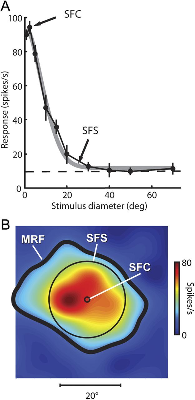
Center and surround extent revealed by the diameter test. A, Responses of an example neuron to spots of different diameters centered on the RF. Filled symbols connected by the black line denote mean neuronal responses at each spot diameter. Vertical black lines are the SE of the mean responses. The horizontal dashed black line shows the neuron's background firing rate. The thick gray line is the descriptive fit to the DoG from which we extracted the extent of the central SFC and the extent of the peripheral SFS. B, MRF for the same example neuron. The SFC (1.6° diameter) and the SFS (25.2° diameter) are represented by black circles superimposed on the MRF map.

The degree of response reduction was taken as the difference between the curve's maximum and its asymptote, normalized by the curve's peak. We subtracted the baseline firing rate, so reduction >100% was possible if the largest stimuli reduced responses below baseline.

Results

We recorded the activity of FEF neurons that responded to visual stimuli in both hemispheres of one monkey and one hemisphere of another monkey. We studied 183 neurons (93 from monkey Ar and 90 from monkey Fl). We saw no significant difference between the monkeys and have combined their results. We included both visual and visuomovement cells, as long as there was a clear visual response from the neuron.

Minimum response field maps of FEF neurons

We were able to map the MRF of 22 neurons using the spot mapping test and constructed gradient maps for each of these cells. Figure 1A–C shows MRF maps for three neurons whose centers were about equidistant from the center of the visual field (about 11°) and whose MRFs substantially overlapped. These x–y plots represent the magnitude of neuronal responses when spots of light were presented at different locations in and around each RF. The relationship between color and response magnitude is shown in the color bar to the right of each plot. Note that the extent of the stimulus grid was adjusted according to MRF size. For each MRF, responses were strongest near the center and gradually tapered off toward the MRF boundary, which is represented by the solid black line in each plot (where neuronal activity reached 2 SD above the background firing rate). Figure 1D provides a direct qualitative comparison of the size and shape of the three maps by superimposing the three contour lines from A–C and illustrates the variability we encountered when mapping MRFs in FEF.

Figure 1.

Variability of spot mapped minimum response field extent. A–C, Visual receptive field maps of three sample FEF neurons. Maps are based on responses to spots flashed at 49 locations on an evenly spaced seven-by-seven grid while the monkey fixated. The black lines on each map are the outline of the MRF extent (see Materials and Methods, Data analysis). D, Outline of the three MRFs from A–C at their actual locations in the visual field. E, MRF extent of 25 neurons (15 from monkey Ar, circles; 10 from monkey Fl, squares) as a function of eccentricity. The MRF areas from A–C are plotted as open symbols and are labeled accordingly.

Figure 1E shows the relationship between MRF size and eccentricity derived from the 22 individual MRF spot maps. The area of the visual MRFs (the region within the boundary contour line) is plotted as a function of MRF eccentricity. The open symbols represent the three MRFs in Figure 1A–C (as indicated by the corresponding letters). The relationship between MRF eccentricity and MRF size was not significant (r = 0.06, p = 0.75), because there was substantial variability in MRF sizes found at each eccentricity.

In summary, the 22 neurons we measured with the spot mapping test all had large, excitatory MRFs that decreased in strength from the center to the periphery. The shape of the excitatory MRF was frequently irregular, but not drastically so, and had a generally circular structure that facilitated our further study of the interaction of this excitatory region with any surround.

Sizes of excitatory summation field centers and suppressive summation field surrounds

For 183 neurons we attempted to measure the RF center by recording neuronal responses to spots of light with different diameters centered on the RF (diameter test from Materials and Methods). Figure 2A shows the responses of an example neuron to the diameter test. Points and vertical error bars represent the means and SEs of responses to the spots of light of each diameter along the horizontal axis. The horizontal black dashed line shows the background rate for this cell (9.7 spikes per second). The thick gray line represents the empirical fit to the DoG curve (Rodieck, 1965) (see Materials and Methods). The DoG curve provided a good fit to these data (Pearson's χ² test, p < 0.001), and we used the fit curve to estimate the size of the SFC, the size of the SFS, and the degree of response reduction. Center and surround diameters were 1.6 and 25.2°, respectively. For the largest stimuli, responses reduced 96% for this neuron.

Keep in mind that the SFC and SFS are simply measurements of the response curves derived from the DoG fit to the data. Their interpretation depends on the aspects of the stimuli to which the neurons are responding. Schall et al. (1995) showed that FEF neurons responded equally well to bright spots or dark spots, suggesting that luminance is not the sole driving factor for these neurons. If FEF neurons respond to, for example, contrast edges rather than luminance, then responses would diminish as the stimulus, the contrast edge, moves to the insensitive RF periphery as the spot grows. In this case, the reduction of response would be due to the withdrawal of the stimulus away from the RF rather than its encroachment on a suppressive surround, and we would expect the SFS to be similar in extent to the MRF. So far our data cannot rule out such a possibility, but forthcoming results will address this issue.

Figure 2B also shows the MRF for this example neuron. Superimposed on the MRF map is a small circle representing the extent of this neuron's SFC and a larger circle showing the extent of the SFS. For this neuron, larger stimuli extending past the 1.6° wide SFC reduced responses. For all neurons in our sample, visual responses decreased with the largest spot sizes in the diameter test. Note, however, that due to the large diameter used and the limited size of the screen (74 × 56°), the edges of the largest stimuli often extended past the visible area of the screen, resulting in large, virtually uniform areas of luminance that would therefore elicit identical responses for stimuli with the largest diameters. For the majority of neurons (158 of 183), the DoG curve provided an acceptable fit (Pearson's χ² test, p < 0.05) to the data obtained from the diameter test.

Using measurements obtained from the significant DoG fits (n = 158, 87 from monkey Ar and 71 from monkey Fl), Figure 3 shows the size of the SFC (Fig. 3A) and the size of the SFS (B) for each neuron as a function of RF eccentricity. The increase in both SFC and SFS extent with eccentricity was significant (r = 0.35 and p < 0.001 for the central SFC; r = 0.52 and p < 0.001 for the outlying SFS). The loose relationship between extent and eccentricity reached significance in the diameter test (Fig. 3A) but not in the spot mapping test (Fig. 1E), most likely due to the larger number of neurons sampled in the former (n = 158) than in the latter (n = 22), as similar degrees of variability in extent were observed in both tests.

Figure 3.

Summaries of RF characteristics from the diameter test. A, Excitatory SFC diameter versus RF eccentricity for 158 FEF neurons. The dashed line is the least squares linear fit to the data. B, Suppressive SFS extent versus RF eccentricity for our sample of FEF neurons. The dashed line is the least squares linear fit to the data. C, Distribution of the degree to which responses were suppressed by the RF surround. From the DoG curve fit to the diameter test data for 158 neurons, we subtracted the background rate from the curve and then calculated suppression as the percentage that the maximum response was reduced by the largest stimuli. Suppression >100% meant responses were suppressed below the background rate. D, Distribution of relative surround sizes for the 158 neurons. Relative surround size was calculated as SFS diameter/SFC diameter.

The histogram in Figure 3C summarizes response reduction across the sample of neurons for which the DoG provided a significant fit. Maximal stimulation of the RF periphery resulted in a mean decrease of 84% in visual responses across the population. Interestingly, responses in 28% of the neurons (n = 44) were reduced below the background firing rate (i.e., reduction >100%), indicating the existence of a suppressive influence. There was no significant relationship between response reduction and eccentricity (r = 0.11, p = 0.39), as the reduction was uniformly distributed across eccentricity. Nor was there a correlation between response reduction and SFS diameter (r = −0.09, p = 0.25).

If FEF neurons respond to a contrast border rather than luminance, as introduced above, then the largest spots would approximate the absence of a stimulus since the contrast edges would be in the far periphery, and we would expect firing rates very near to baseline. Although this was true for many of the cells we recorded, most neurons had firing rates different from baseline for the largest spots (Fig. 3C), suggesting that the contrast border was not a solitary driving force. In addition, the suppression of responses below baseline for many neurons indicates that responses were reduced by a suppressive influence rather than simply by removal of excitation.

We expressed the relative size of the surround as the SFS diameter divided by the SFC diameter. Figure 3D shows the distribution of relative surround sizes. For our sample, outlying SFS diameters were, on average, 12.8 times larger than the central SFC.

Of the 25 neurons for which we were able to obtain MRFs, there were 19 on which we also performed the diameter test. Since MRFs were roughly circular in shape, we took the diameter of the MRF as the diameter of the circle that had the same area as the MRF. Figure 4A shows the MRF diameter versus the excitatory SFC diameter for these 19 neurons. All of the points fall above the unity diagonal, meaning that all of the excitatory MRFs were larger than the excitatory SFCs. MRF diameters were, on average, 12.1 ± 9.7 times greater than SFC diameters. Of particular interest, MRF extent was more in agreement with the larger SFS, being 1.1 ± 0.85 times the SFS diameter (Fig. 4B). This indicates (as suggested in Fig. 2B) that the SFS began and often ended completely within the bounds of the excitatory MRF. If the contrast boundary were the dominant stimulus for these RFs, we would have expected a much stronger correlation between the MRF and the SFS than that seen in Figure 4B. The lack of such significant correlation tells us again that the contrast edge was not necessarily the exclusive driving stimulus for the visual responses we recorded, and response reduction was not merely the result of loss of excitation.

Figure 4.

Comparison of minimum response fields and summation fields. A, MRF diameter versus SFC diameter for 19 neurons (4 from monkey Ar; 15 from monkey Fl). MRFs were, on average, 12.1 times larger than the excitatory SFC. B, MRF diameter versus SFS diameter for the same 19 neurons. Excitatory MRFs were, on average, 1.1 times larger than the suppressive SFS.

In summary, the measured extent of the excitatory RF was dependent on the type of stimulus used. Probing with small spots across the RF revealed a large excitatory region (MRF), whereas using an expanding spot resulted in smaller estimates of excitatory RF extent (SFC). Cells responding to the border of the expanding spot would produce similar estimates of MRF and SFC, but we observed no strong correlation between these two measurements (Fig. 4B). Also, we observed suppression below the baseline firing rate for stimuli extending into the periphery (Fig. 3C), which suggests a sizable suppressive influence.

Nonlinear interaction between excitatory center and suppressive surround

The diameter test revealed a reduction in response for larger stimuli common to all the RFs we measured in FEF. As shown in Figure 2, when expanding a central spot past the optimal diameter, responses were reduced even though discrete probing of this “suppressive” region when mapping the MRF produced excitation.

For some neurons in the diameter test, responses were completely eliminated (Fig. 2). For these neurons, it was possible that any peripheral suppressive influence extended farther than we calculated because surround suppression saturated. To examine the influence of the surround in this region of complete response reduction, we needed to differentially stimulate the RF periphery while generating a strong response from the center. Therefore, we placed a relatively small stimulus in the RF center that generated a vigorous response and then stimulated the surround with an annulus. While keeping the outer diameter of the annulus constant at 70°, we varied the inner diameter to engage different peripheral regions of the surround (see Materials and Methods, Annulus test).

Figure 5 shows the responses of our example cell (from Fig. 2) during the annulus test. We stimulated the RF center with a spot of 1° diameter, which was smaller than the central SFC but still elicited a near-maximal response. The annulus stimulating the surround had a constant outer diameter of 70°, and the abscissa in Figure 5 indicates the varying inner diameter of the surround annulus. Open symbols and vertical error bars represent the means and SEs of responses to the central spot in the presence of annuli with different inner diameters. Below the plot are example stimuli (not to scale) to illustrate the withdrawal of the annulus from the central spot. When the inner diameter of the annulus was 1° (the same as the diameter of the central spot), the center spot and the annulus formed a continuous single large spot 70° in diameter. From Figure 2, we would expect the response to this large 70° stimulus to be at or near baseline, and this is just what we observed. As the annulus inner diameter increased and the annulus withdrew from the central spot, the visual response steeply increased, as would be expected when the annulus stimulated less and less of the suppressive surround. Pulling the annular inner diameter further away, however, produced an unexpected decrease in neuronal response (Fig. 5) (inner diameters from 5 to 15°), even though we were supposedly removing suppression by stimulating less of the suppressive surround. The expected pattern of increasing responses with increasing annulus inner diameter resumed past the 15° mark until the annulus disappeared (at 70° inner diameter) leaving just the central spot. Rather than just obtaining a better estimate of surround extent, the annulus test uncovered aspects of the RF that could not be observed with just an expanding spot.

Figure 5.

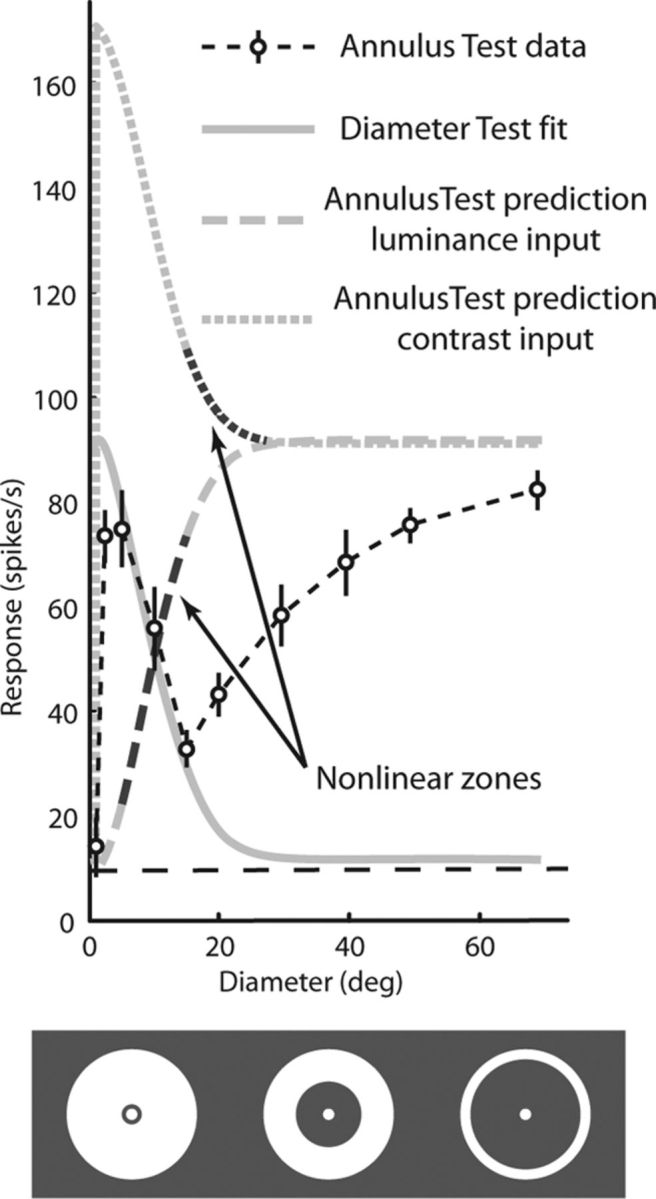
DoG model fails to predict responses to the annulus test. Responses to the annulus test for the same example neuron shown in Figure 2. Open symbols connected by the dashed black line are the mean neuronal responses to a central spot in the presence of an annulus with the annular inner diameter indicated on the abscissa. Vertical lines denote the SE of the mean responses. The horizontal dashed black line is the background firing rate. The progression of annulus expansion is illustrated (not to scale) below the plot. The gray solid line is the DoG fit to the diameter test for the same neuron (from Fig. 2). Fitting to either stimulus luminance or stimulus contrast yielded the same curve. The lower gray dashed line is the prediction of responses to stimulus luminance in the annulus test made by the same DoG that described the data in the diameter test. The top gray dotted line is the prediction of responses to the stimulus edges in the annulus test made by the same DoG that described the data in the diameter test. The darker regions of both these curves indicate the nonlinear zone, where the model prediction differed in sign from the data (e.g., the model predicted an increase, whereas the data showed a decrease).

We previously fit our data to a DoG curve because it empirically provided excellent fits to the data from the diameter test. Implicit in our fits to a DoG curve is the idea that these data can be described by the interaction between two components: one excitatory and one suppressive. If we now adopt the DoG as a model of neuronal activity rather than just a description of a pattern of responses, we can consider the Gaussian components of the DoG to represent the RF center and surround, and the resulting curve to be the consequence of interactions between these two components. Moreover, we can use such a model to predict responses to the stimuli in the annulus test.

The solid gray line in Figure 5 represents the DoG fit to the data from the diameter test (the same as in Fig. 2A). The bottom dashed gray line shows the prediction of this DoG model (determined by the fit to the diameter test) to the extent of stimulus luminance used in the annulus test. To fit the responses to the stimuli used in the annulus test to the DoG model, we calculated the linear activity L of the center and surround components as follows:

where L(r_c) is the linear response to the central spot with radius r_c, L(r_o) is the linear response to a spot with radius r_o, and L(r_i) is the response to a spot with radius r_i. The quantity [L(r_o) − L(r_i)] therefore represents the linear response to just the annulus with an inner radius r_i and an outer radius r_o (for calculation of L, see Materials and Methods). As the annulus pulls away from the RF center, it should stimulate less of the suppressive surround, and responses should monotonically increase as the inner diameter of the annulus leaves the suppressive surround (as the dashed fit curve shows). Of course, this is not what we observed. Responses to the annular stimuli differed greatly from the DoG prediction, and for some RF regions showed response increases where the DoG predicted decreases (and vice versa).

The prediction of the model becomes obvious when we consider how the annular stimulus corresponds to the expanding spot stimulus. As the diameter of the spot increases, the luminance expands into more peripheral regions of the RF. As the annulus dilates, luminance is withdrawn from these same regions. So the difference between the spot and the annulus is the difference between the addition of luminance and the removal of the same luminance. Thus we would expect changes in responses in the two curves to mirror each other; as one curve rises the other should fall. It is immediately apparent from the annulus test data that this is not the case.

Perhaps, as discussed before, luminance is not what drives the visual responses of FEF neurons. We fitted another version of the DoG model that used a 1° wide annulus centered on each contrast border as the stimulus, representing RF components that respond to contrast edges rather than luminance (see above for calculation of responses to annuli). A simple DoG using this alternate input yielded the same fit to the diameter test as the luminance DoG (the same solid gray curve). But the prediction of this model to the data from the annulus test yielded the upper dotted gray curve in Figure 5. This prediction is also readily apparent from the stimuli. In this case, the contrast edges from the expanding spot and the dilating annulus bestow the same driving input. The only difference between the two curves should be the response to the central spot in the annulus test; the curves should rise and fall together, displaced by the constant response to the edge of the central spot. Again, this is not what we observed.

Both DoG models, one using stimulus luminance and the other using contrast edges, make opposite predictions as to the responses from the annulus test. In both cases, there are regions of the RF that respond in a manner contrary to the simple RF prediction, leading us to ask whether these regions of the RF are excitatory or inhibitory. The answer is, of course, that it depends on the stimulus, as Bair (2005) recognized for visual receptive fields in general. This is a characteristic of the RF that cannot be represented by the linear activation of the center and surround components in the DoG model in which each region of the RF is exclusively excitatory or suppressive, so we designate this region of the RF the nonlinear zone: a region of the RF that is either excitatory or suppressive depending on what other areas of the receptive field are being stimulated. Note that the nonlinear zone differed depending on which aspect of the stimulus we assumed to be driving the neurons (luminance or contrast), but either assumption revealed a nonlinear zone of the RF, suggesting interesting interactions between center and surround.

The widespread existence of this nonlinear zone indicates that the excitatory center and the suppressive surround of FEF RFs do not respond in a simple linear manner. A region of the RF that can be either excitatory or suppressive (the nonlinear zone) is impossible to model with a simple DoG with center and surround mechanisms that respond linearly to the stimulus configuration. Obviously, something else is required.

Modeling the nonlinear characteristics of the FEF RF

Although the DoG model provided an adequate description of the responses to an expanding spot, it routinely failed to account for the pattern of responses to the expanding spot and the dilating annulus, as illustrated above. Following Cavanaugh et al. (2002a), we realized that independently modulating the gains of the center and surround mechanisms should allow us account for responses in the nonlinear zone of the RF. We therefore modified the DoG model by independently setting the gains of the center and surround components as a function of the activity of each mechanism. The intuition is that gain should decrease with activation. After some initial experimentation with our model, we noticed that gains did indeed decrease with activation, but eventually reached an asymptotic level. We therefore chose to have the gains of the center and surround mechanisms decay exponentially with activation, although any of several functions that monotonically decrease to a fixed lower limit may have worked as well. For the center and surround components of our model, we chose to modulate the gains according to the following equation:

in which the mechanism gain g is set by an inverse exponential with a vertical offset α (from 0 to 1) and a decay factor of λ (yielding maximum value of 1). As in the simple DoG model, L is the summed activity of the mechanism covered by the stimulus. This gives rise to a new model that we call the modulated gain model and has the following form:

Note the similarity to the original DoG (Eq. 1) described in Materials and Methods.

The differential performance of both models is illustrated in Figure 6 for both types of stimulation: luminance and contrast. The responses of two different neurons (the columns in Fig. 6) are shown fit to the DoGs (luminance-driven in the first row, contrast-driven in the second). Figure 6A shows the fit of the DoG model to data from the diameter test and the annulus test for same example neuron used in Figures 2 and 5. The data for both tests were fit simultaneously to the DoG model (unlike in Fig. 5, where we fit the data from the diameter test only and used the parameters to predict the responses to the annulus). The fit to the same model using the contrast borders as input is shown in Figure 6B. Neither model makes very good predictions of the data.

Figure 6.

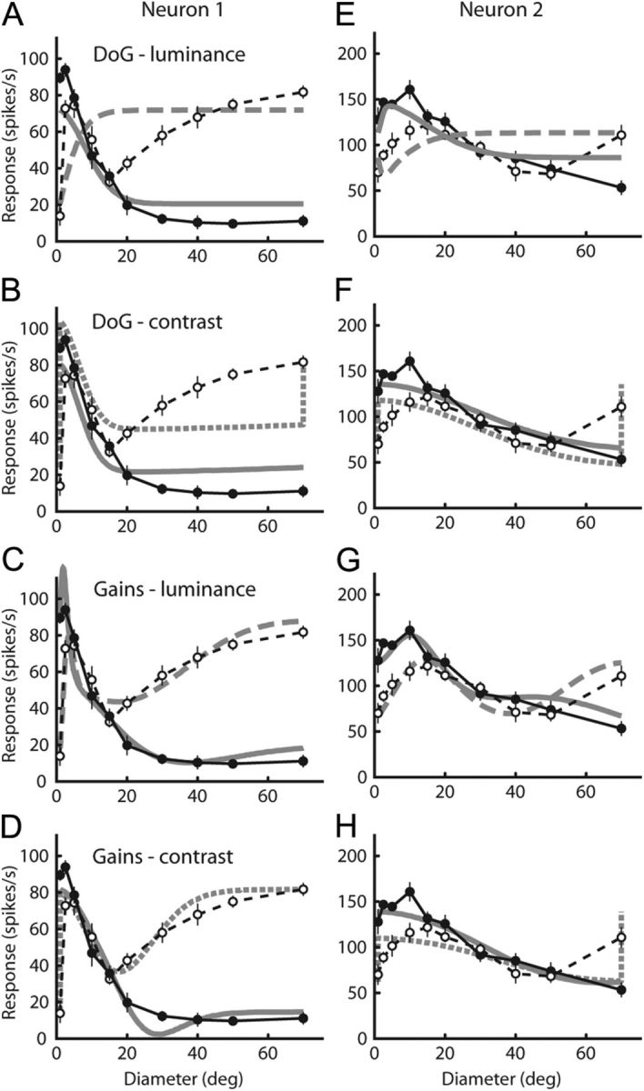
A–H, Fits of the DoG model and modulated gains model to two example neurons (neuron 1, A–D; neuron 2, E–H). A and E are fits to the simple DoG with luminance input. B and F are fits to the simple DoG with contrast (edge) input. C and G show fits to the modulated gains model with luminance input. D and H show fits to the modulated gains model with contrast (edge) input. For each neuron, data from both tests were fit simultaneously to each model. Filled symbols connected by solid black lines are data from the diameter test, and open symbols connected by dashed black lines are data from the annulus test. For each panel, the thick gray line is the model's prediction of the diameter test data, and the thick dashed gray line is the prediction of the same model to the annulus test data. The sum squared error and E_N (in parentheses) for each panel is as follows: A, 1.1 × 10⁵ (7054); B, 4.3 × 10⁴ (2871); C, 2860 (260); D, 1360 (124); E, 2.1 × 10⁵ (1.4 × 10⁴); F, 3.5 × 10⁴ (2345); G, 1.2 × 10⁴ (1072); H, 2.4 × 10⁴ (2218). A smaller E_N value indicates the model that better accounted for the data, taking into account the number of model parameters.

The fit to the modulated gain model with luminance input is shown in Figure 6C. At first glance, the fit is much better than that of the DoG model in Figure 6A. The modulated gain model now correctly predicts responses where the simple DoG failed. We also modulated the gains of the model with contrast input (Fig. 6D) and achieved fits that were also able to more accurately represent the responses. But was the addition of extra parameters worth the improvement in fit quality?

By adding the independently varying gain values for both the center and surround, we have four more parameters than the regular DoG model (two for the center and two for the surround), so obviously the modulated gain model fit the data better. We quantified the benefit of adding the extra parameters by calculating an error quantity that took into account the additional parameters. We calculated a normalized error E_N by dividing each sum squared error (assuming normal distribution of errors) between the data and the fit by the number of degrees of freedom in each model (Hoel et al., 1971; Cavanaugh et al., 2002b). The normalized errors E_N for the two models were therefore directly comparable.

The normalized error E_N for the DoG fit in Figure 6A was 7054, whereas the modulated gain model in Figure 6C resulted in a much smaller E_N of 260, indicating a vast improvement well worth the additional gain parameters. Using contrast input, the normalized error E_N changed from 2871 to 124 when the gains changed with activation (Fig. 6B,D). Figure 6E–H shows similar data from another neuron. Again, modulating the component gains with activation significantly improved the fit to the data.

For the 153 neurons that we fit to the models, Figure 7 compares the normalized error E_N. For luminance input, Figure 7A shows how E_N changes when the gains of the model are modulated with activation. Most points fall well below the unity diagonal, indicating a lower E_N for the modulated gain model (paired t test, p < 0.001). When using the contrast borders as the input, E_N also significantly improved (Fig. 7B) (p = 0.001). In fact, either model with modulated gains did better than the simple DoG, regardless of the input used (p < = 0.003). Although the DoG models frequently failed to account for certain characteristics of the data (as in Fig. 6A,B), using the contrast border as input to the DoG typically yielded better results than the luminance input (p = 0.002). This trend disappeared, however, once the gains were modulated. Figure 7C shows that there is no overall difference in fit between luminance input and contrast input once the gains are modulated (p = 0.966), indicating that the modulation of the gains is more important than the choice of driving input in accounting for the responses of these neurons.

Figure 7.

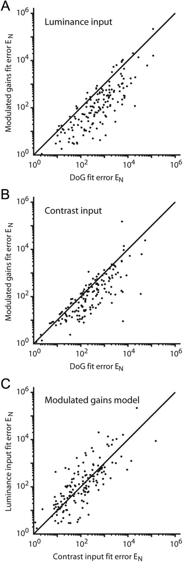
Comparison of DoG model and modulated gains model performance. For each neuron, compare the normalized errors E_N for two model instances to determine which model better accounted for the data. A, For luminance input, E_N for the modulated gains model versus E_N for the simple DoG is shown. The clustering of points below the unity diagonal indicates that E_N was almost always lower for the modulated gains model than for the DoG model. B, For contrast (edge) input, E_N for the modulated gains model versus E_N for the simple DoG is shown. The clustering of points below the unity diagonal indicates that again E_N was almost always lower for the modulated gains model than for the DoG model. C, For the modulated gains model, E_N for luminance input versus E_N for contrast input is shown. When modulating gains, both inputs produced similar results.

Discussion

We discovered a ubiquitous suppressive surround in FEF neurons that was not evident when measuring the MRF with small spots. Consequently, the extent of the excitatory RF center was strongly dependent on the stimuli used to map the RF. By simultaneously stimulating different regions of the RF, we observed that some regions of the RF could be excitatory or suppressive depending on stimulus configuration. A standard DoG model was incapable of accounting for the peculiar features of our data, so we modified a DoG model by changing the gains of the center and surround components independently with a simple inverse exponential. This modulation of gain resulted in a model that effectively represented the more interesting and counterintuitive aspects of our data.

Suppressive surrounds and RF structure

Suppressive surrounds have been found in a number of areas of visual cortex, but have not been systematically studied in FEF. The presence of such suppression, however, might have been observed in FEF by Schall et al. (1995), who compared visual responses to stimuli in the RF with and without distractor stimuli. Overall they observed significantly stronger responses to lone stimuli than to stimuli with distractors, a difference possibly attributable to surround suppression. We are unaware of any other studies that have tested for the presence, magnitude, and extent of FEF suppressive surrounds.

The anomalies we found in FEF RF surrounds were similar to those found in nonclassical surrounds, particularly those studied extensively in V1 (Cavanaugh et al., 2002a). There are possibly two major differences between our data from FEF and the effects observed in V1 if we consider stimulus luminance to be driving the FEF neurons. First are the differences in measured RF extent. In V1, MRFs were approximately one-third the size of excitatory RFs analogous to our SFC (Walker et al., 1999; Cavanaugh et al., 2002b), whereas in FEF MRFs are about 12 times larger than the excitatory SFC (Fig. 4A). The second difference concerns the location of the nonlinear zone. The nonlinear zone in FEF falls within the MRF, whereas in V1 it falls outside this region. Note that if FEF neurons were responding to the contrast borders of our stimuli, the MRF and SFS would be in agreement, and the nonlinear zone would not necessarily fall outside this excitatory influence.

Figure 8 demonstrates how apparently disparate sets of observations can arise from the same class of model. We represent the V1 RF with a small center excitatory mechanism in the left column and FEF with a large center in the right column. The solid curves represent the weighted center and surround mechanisms, and the dashed curve is the resulting RF profile. Assuming that probing the RF periphery with small spots does not substantially alter the gains of the mechanisms, the excitatory MRFs (dark shaded areas) will be revealed as shown in Figure 8, A and B. This measurement of RF extent is carried downward into the other panels for comparison as the lighter shaded area. Large stimuli will reduce the gains of both mechanisms, but the gains will decrease differently for each mechanism, resulting in a different balance of center and surround influence. If the relative influence of V1 surrounds decreases more than FEF surrounds, then the balance of center and surround activity in response to larger stimuli (as in the diameter test) would produce the results in Figure 8, C and D. The relatively weaker V1 surround results in SFCs larger than MRFs, but the opposite occurs in FEF where we observe SFCs smaller than the MRF. Strong surround stimulation (as in the annulus test) reduces surround gain even further in Figure 8, E and F, where we show the RF profiles from C and D as the gray dashed curves, and the RF profile with reduced surround gain as the black dashed curves. Further reducing surround gain permits previously suppressive parts of the RF to become excitatory, thus revealing the nonlinear zone (black shaded areas). Moreover, the nonlinear zone appears outside the V1 MRF, but completely within the MRF in FEF. Clearly, such differences need not suggest a different type of surround, but may simply reflect a different balance between excitation and suppression with stimulation, as just demonstrated.

Figure 8.

Modulating gain changes measured RF extent and creates the nonlinear zone. A, C, E, DoG model with a relatively small center component representing V1. B, D, F, DoG model with larger center component representing FEF. A and B show how probing the RF with small spots reveals a small excitatory MRF in V1 and a larger excitatory MRF in FEF. The relative strengths of the center and surround components are represented by the solid curves. The dashed RF profile is simply the difference of the two Gaussian components. The dark shaded area represents the measured MRF. This MRF extent is carried down through both columns of panels in the lighter shaded region for comparison. C and D illustrate how a large central stimulus as in the diameter test could change the relative strengths of the center and surround differently in V1 and FEF, yielding a larger SFC in V1 and a smaller SFC in FEF. Lines and shading carry the same meaning as in A and B. E and F illustrate the creation of the nonlinear zone. The gray dashed curves are the RF profiles from C and D above. The black dashed curve in each panel is the proposed RF profile in the presence of substantial surround stimulation, as in the annulus test, which would attenuate the surround and give the center relatively more strength. The nonlinear zone is indicated by the black shaded regions, in which the RF is excitatory with surround stimulation but inhibitory with center stimulation. Note the location of the nonlinear zone relative to the lightly shaded region representing MRF extent.

Modeling overlapping but independent center and surrounds

It is obvious that a simple DoG model cannot account for the nonlinear zone, as a DoG requires that each part of the RF must be exclusively excitatory or suppressive. We have shown that independently varying the center and surround gain produces nonlinear zones.

Although we used circularly symmetrical stimuli, we did not confirm that the FEF surrounds were in fact symmetrical. Our interpretations would not change, however, even assuming asymmetrical surrounds. As long as the center and surround components are spatially constant, their actual shape is immaterial since each region of the static RF has a consistent balance between center and surround influences that should either increase or decrease responses. The fact remains that stimulating certain regions of the RF (whether by luminance or contrast) results in either increased or decreased responses, achieved here by independent modulation of the component gains.

Because modulating the gains in our model allowed us to account for responses to both luminance and contrast, we propose that such an approach could model responses to any class of stimulus. Simply consider the center and surround components as envelopes of activation that are selective to the relevant stimulus attributes. This scheme is implicit even when modeling simple cells in V1, where the center Gaussian is actually the envelope of a Gabor filter (Movshon et al., 1978) representing the spatial frequency and orientation preferences of the neuron. Once the Gaussian components are properly characterized, the responses to various stimuli can be modeled by modulating the gains of the center and surround.

One of our goals was to determine the manner in which the gains of the center and surround changed with stimulation. Modulating the gains by having them reduce exponentially permitted our model to account for the nonlinear zone of FEF RFs. It is expected that the same effects seen in the nonclassical surrounds of V1 neurons could be represented by modulating center and surround gains in the same manner.

We suggest that this form of gain modulation may be a universal feature of visual RFs. A number of RF characteristics can be explained by combining the same center and surround mechanisms, varying only in selectivity, extent, and gain modulation. One intriguing consequence of such a simple approach is a blurring of the distinction between classical and nonclassical RFs. The difference may simply be which regions of the RF are revealed or hidden by certain stimuli. Another distinction made ambiguous is between excitatory and inhibitory regions of the RF. Large regions of visual RFs initially characterized as being excitatory can turn suppressive simply by presenting different stimuli. This might be particularly relevant to experiments examining stimulus context, such as those in V1 and MT (Albright and Stoner, 2002; Hunter and Born, 2011), since variations in neuronal response may result from stimulus-driven changes in the measured RF, but the relevance of such conjectures remains to be explored.

Possible relation of suppressive surrounds to behavior modulations

All of the FEF neurons we studied showed suppressive surrounds, but all were examined in a passive state; that is, the monkey was not rewarded for discriminating changes in stimuli, but simply for maintaining fixation. In contrast, most studies exploring the activity of FEF neurons required the monkey to perform tasks in which the stimulus was the focus of attention, the object of a visual search, or the target of a saccade. One possibility is that some behaviorally induced modulations of visual responses seen in FEF and other areas result from changes in the relative strengths of RF center and surround mechanisms (Ghose, 2009). For example, one of the first demonstrations of behavioral effects on neuronal responses in FEF was an enhanced visual response of a stimulus when it became the target of a saccade (Mohler et al., 1973; Bruce and Goldberg, 1985). This could be facilitated by relatively increasing the gain of the excitatory center or decreasing the gain of the suppressive surround. Modulation of suppressive surrounds with attention has been found in V4 neurons where attention to one stimulus in the center of the RF reduced the effect of distractors falling in the surround (Sundberg et al., 2009). Similarly for neurons in the lateral intraparietal area of parietal cortex, when one spot becomes the target of a saccade, the responses to other stimuli distant from the target are suppressed (Falkner et al., 2010).

It is evident that changes in visual salience can result from modulating the relative strength of the suppressive surround. It is interesting to speculate that the straightforward regulation of center and surround gains that yields complex responses to different stimuli in a passive fixation task may be the same mechanism through which attention works in more active tasks to modify visual responses in higher visual areas.

References

- Albright TD, Stoner GR. Contextual influences on visual processing. Annu Rev Neurosci. 2002;25:339–379. doi: 10.1146/annurev.neuro.25.112701.142900. [DOI] [PubMed] [Google Scholar]
- Allman J, Miezin F, McGuinness E. Stimulus specific responses from beyond the classical receptive field: Neurophysiological mechanisms for local–global comparisons in visual neurons. Annu Rev Neurosci. 1985a;8:407–430. doi: 10.1146/annurev.ne.08.030185.002203. [DOI] [PubMed] [Google Scholar]
- Allman J, Miezin F, McGuinness E. Direction- and velocity-specific responses from beyond the classical receptive field in the middle temporal visual area (MT) Perception. 1985b;14:105–126. doi: 10.1068/p140105. [DOI] [PubMed] [Google Scholar]
- Bair W. Visual receptive field organization. Curr Opin Neurobiol. 2005;15:459–464. doi: 10.1016/j.conb.2005.07.006. [DOI] [PubMed] [Google Scholar]
- Ben Hamed S, Duhamel JR, Bremmer F, Graf W. Representation of the visual field in the lateral intraparietal area of macaque monkeys: a quantitative receptive field analysis. Exp Brain Res. 2001;140:127–144. doi: 10.1007/s002210100785. [DOI] [PubMed] [Google Scholar]
- Bruce CJ, Goldberg ME. Primate frontal eye fields. I. Single neurons discharging before saccades. J Neurophysiol. 1985;53:603–635. doi: 10.1152/jn.1985.53.3.603. [DOI] [PubMed] [Google Scholar]
- Cavanaugh JR, Bair W, Movshon JA. Selectivity and spatial distribution of signals from the receptive field surround in macaque V1 neurons. J Neurophysiol. 2002a;88:2547–2556. doi: 10.1152/jn.00693.2001. [DOI] [PubMed] [Google Scholar]
- Cavanaugh JR, Bair W, Movshon JA. Nature and interaction of signals from the receptive field center and surround in macaque V1 neurons. J Neurophysiol. 2002b;88:2530–2546. doi: 10.1152/jn.00692.2001. [DOI] [PubMed] [Google Scholar]
- Crist CF, Yamasaki DS, Komatsu H, Wurtz RH. A grid system and a microsyringe for single cell recording. J Neurosci Methods. 1988;26:117–122. doi: 10.1016/0165-0270(88)90160-4. [DOI] [PubMed] [Google Scholar]
- Desimone R, Schein SJ. Visual properties of neurons in area V4 of the macaque: sensitivity to stimulus form. J Neurophysiol. 1987;57:835–868. doi: 10.1152/jn.1987.57.3.835. [DOI] [PubMed] [Google Scholar]
- Falkner AL, Krishna BS, Goldberg ME. Surround suppression sharpens the priority map in the lateral intraparietal area. J Neurosci. 2010;30:12787–12797. doi: 10.1523/JNEUROSCI.2327-10.2010. [DOI] [PMC free article] [PubMed] [Google Scholar]
- Gegenfurtner KR, Kiper DC, Fenstemaker SB. Processing of color, form, and motion in macaque area V2. Vis Neurosci. 1996;13:161–172. doi: 10.1017/s0952523800007203. [DOI] [PubMed] [Google Scholar]
- Ghose GM. Attentional modulation of visual responses by flexible input gain. J Neurophysiol. 2009;101:2089–2106. doi: 10.1152/jn.90654.2008. [DOI] [PMC free article] [PubMed] [Google Scholar]
- Gilbert CD, Wiesel TN. The influence of contextual stimuli on the orientation selectivity of cells in primary visual cortex of the cat. Vision Res. 1990;30:1689–1701. doi: 10.1016/0042-6989(90)90153-c. [DOI] [PubMed] [Google Scholar]
- Hays AV, Richmond BJ, Optican LM. A UNIX-based multiple process system for real-time data acquisition and control. WESCON Conf Proc. 1982;2:1–10. [Google Scholar]
- Hoel P, Port S, Stone C. Introduction to statistical theory. Boston: Houghton-Mifflin; 1971. [Google Scholar]
- Hunter JN, Born RT. Stimulus-dependent modulation of suppressive influences in MT. J Neurosci. 2011;31:678–686. doi: 10.1523/JNEUROSCI.4560-10.2011. [DOI] [PMC free article] [PubMed] [Google Scholar]
- Joiner WM, Cavanaugh J, Wurtz RH. Modulation of shifting receptive field activity in frontal eye field by visual salience. J Neurophysiol. 2011;106:1179–1190. doi: 10.1152/jn.01054.2010. [DOI] [PMC free article] [PubMed] [Google Scholar]
- Mohler CW, Goldberg ME, Wurtz RH. Visual receptive fields of frontal eye field neurons. Brain Res. 1973;61:385–389. doi: 10.1016/0006-8993(73)90543-x. [DOI] [PubMed] [Google Scholar]
- Movshon JA, Thompson ID, Tolhurst DJ. Receptive field organization of complex cells in the cat's striate cortex. J Physiol. 1978;283:79–99. doi: 10.1113/jphysiol.1978.sp012489. [DOI] [PMC free article] [PubMed] [Google Scholar]
- Rodieck RW. Quantitative analysis of cat retinal ganglion cell response to visual stimuli. Vision Res. 1965;5:583–601. doi: 10.1016/0042-6989(65)90033-7. [DOI] [PubMed] [Google Scholar]
- Schall JD. On the role of frontal eye field in guiding attention and saccades. Vision Research. 2004;44:1453–1467. doi: 10.1016/j.visres.2003.10.025. [DOI] [PubMed] [Google Scholar]
- Schall JD, Hanes DP, Thompson KG, King DJ. Saccade target selection in frontal eye field of macaque. I. Visual and premovement activation. J Neurosci. 1995;15:6905–6918. doi: 10.1523/JNEUROSCI.15-10-06905.1995. [DOI] [PMC free article] [PubMed] [Google Scholar]
- Sommer MA, Wurtz RH. Composition and topographic organization of signals sent from the frontal eye field to the superior colliculus. J Neurophysiol. 2000;83:1979–2001. doi: 10.1152/jn.2000.83.4.1979. [DOI] [PubMed] [Google Scholar]
- Sundberg KA, Mitchell JF, Reynolds JH. Spatial attention modulates center-surround interactions in macaque visual area v4. Neuron. 2009;61:952–963. doi: 10.1016/j.neuron.2009.02.023. [DOI] [PMC free article] [PubMed] [Google Scholar]
- Walker GA, Ohzawa I, Freeman RD. Asymmetric suppression outside the classical receptive field of the visual cortex. J Neurosci. 1999;19:10536–10553. doi: 10.1523/JNEUROSCI.19-23-10536.1999. [DOI] [PMC free article] [PubMed] [Google Scholar]