Interaction Terms in Nonlinear Models

Abstract

Objectives

To explain the use of interaction terms in nonlinear models.

Study Design

We discuss the motivation for including interaction terms in multivariate analyses. We then explain how the straightforward interpretation of interaction terms in linear models changes in nonlinear models, using graphs and equations. We extend the basic results from logit and probit to difference-in-differences models, models with higher powers of explanatory variables, other nonlinear models (including log transformation and ordered models), and panel data models.

Empirical Application

We show how to calculate and interpret interaction effects using a publicly available Stata data set with a binary outcome. Stata 11 has added several features which make those calculations easier. LIMDEP code also is provided.

Conclusions

It is important to understand why interaction terms are included in nonlinear models in order to be clear about their substantive interpretation.

The purpose of this paper is to explain the use of interaction terms in nonlinear models. A paper by Ai and Norton (2003) has received a great deal of attention due to the importance of interaction terms in applied research. However, a number of issues regarding interaction terms continue to be confusing to applied researchers. These issues include understanding the conceptual motivations for including interaction terms in models, defining precisely a policy-relevant marginal effect based on a counterfactual, knowing how to interpret interaction terms graphically in nonlinear models, and knowing how to compute interaction terms with real data.

We begin by explaining the reasons for interest in interaction terms and the effect of adding interaction terms in simple linear regression models. Next, we explain how those effects change when the model is nonlinear. We also present an odds-ratio interpretation of the interaction effects and discuss how to interpret interaction terms in panel data models. In addition, we show three different ways to compute interaction effects in Stata, along with their standard errors. We include LIMDEP code, as well, and illustrate our points using publicly available data from Stata.

Although the material in the body of the text is primarily narrative, we provide Appendix S1 that contains a mathematical presentation of all the points made in the paper. Advanced readers may wish to go directly to Appendix S1.

Background

We assume that the reader is familiar with the basic linear regression model of the form:

(1)

where y is an outcome (dependent) variable, x₁ is an explanatory variable, u is a random error term, and β₀ and β₁ are parameters to be estimated.

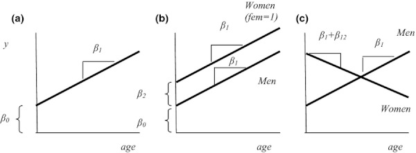
The effect of a one-unit change in x₁—from a specific value of x₁—on E(y|x₁), given byβ₁, is constant over the entire range of x₁. This model is shown in Figure 1a, where both β₀ and β₁ are assumed to be positive and x₁ is a continuous variable such as age. The effect of a one-unit change on the dependent variable is the marginal effect of the explanatory variable on the dependent variable. The marginal effect is obtained by differentiating the conditional expected value of the dependent variable with respect to the explanatory variables: When the explanatory variable is a discrete variable, like sex (male or female) or the presence or absence of a chronic illness, the marginal (or incremental) effect is an arithmetic difference, E(y|x₁ = 1) − E (y|x₁ = 0), rather than a derivative.

Figure 1.

Interaction Terms in Linear Models

Let x₁ be a continuous variable, such as age. Then, add a binary explanatory variable, like female, to the model, which can then be written as follows:

(2)

where age is the subject's age in years and female is coded 1 if the subject is female and 0 if the subject is male. This model with all positive parameters is shown in Figure 1b. Notice that in Figure 1b, the effect of a one-unit change in age on E(y|x), where x refers to the vector of covariates, is the same for men and women and is constant over the entire range of age. The difference in the conditional expected value of y between men and women with respect to age is fully captured by the difference in the y intercept for men and women, estimated by the parameter β₂.

The analyst might hypothesize that the marginal effect of age is different for men and women. Changes in the marginal effect of one variable induced by changes in another variable's value are represented by cross-partial derivatives or differences, also called interaction effects. In some literatures, variables that alter the effect of one variable on another are referred to as modifiers. The hypothesis that female changes the effect of age on E(y|x) (or equivalently that age changes the effect of female on E(y|x)) can be tested by adding an interaction term of the form age × female to the model:

(3)

A model with an interaction effect allows both the intercept and the marginal effect (slope) of age on E(y|x) to be different for men and women (see Figure 1c). At lower values of age, women have higher conditional expected values of y than men, whereas at higher values of age the reverse is true. The marginal effect of age for men is β₁, whereas the marginal effect for women (when female = 1) is β₁ + β₁₂. However, the marginal effect of age on E(y|x) for either men or women is constant over the entire range of age.

If we substitute “treatment group” and “control group” for “women” and “men,” we see that Figure 1b is a model of homogeneous treatment effects with respect to age, whereas Figure 1c is a model of heterogeneous treatment effects with respect to age.

Interaction terms can involve any combination of continuous and discrete explanatory variables. The combination of one continuous variable and one discrete (binary) variable simply facilitates graphical presentation of the model.

Nonlinear Models

We now explain how the interpretation of interaction terms changes when the model is not a simple linear model, but instead is a nonlinear model.

Using a general functional form F(.), we can write the conditional expected value of y to be a general function of the linear index function

(4)

The function F could be the simple linear (identity) function, a logit or probit (normal) transformation, the logarithmic or exponential transformation, or any other nonlinear function of the linear index function. It is important to understand that the issues about interaction terms discussed here apply to all nonlinear models, including log transformation models. In equation (4), letting v = β₀ + β₁x₁ + β₂x₂ + β₁₂(x₁ × x₂), the marginal effect of x₁ on the conditional expected value of y is as follows:

(5)

if x₁ is a continuous variable. Appendix S1 includes detailed calculations of the marginal effects and the cross-partial derivatives for discrete and continuous variables.

In contrast to a linear model (equation 3), the marginal effect of an explanatory variable in a nonlinear model is not constant over its entire range, even in the absence of interaction terms (i.e., β₁₂ = 0). Figure 2 shows a typical binary logit or probit model with a single continuous explanatory variable age (as shown on the right-hand side of equation 1). The dependent variable is the conditional probability that the binary outcome is equal to one, rather than zero. The relationship between age and the conditional probability that y equals 1 is S-shaped, indicating that an additional year of age (e.g., the marginal effect of age) has little effect on the conditional probability that y equals 1 for extremely high and low values of age, but there is a mid-range of age where the effect of an additional year of age is larger. The marginal effect of age is shown by the slope of the lines tangent to the S-shaped curve. In this example, the marginal effects are positive and roughly equal for subjects who are 20 or 40 years old, but nearly zero for subjects who are 70.

Figure 2.

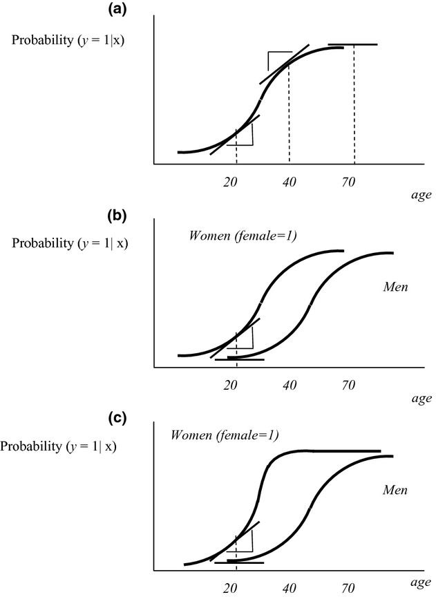
(a) A Logit or Probit Model with a Single Continuous Explanatory Variable (age). (b) A Logit or Probit Model with Continuous (age) and Binary (female) Explanatory Variables. (c) A Logit or Probit Model with Continuous (age) and Binary (female) Explanatory Variables and Their Interaction

The addition of a binary explanatory variable like female to the logit or probit model (as shown on the right-hand side of equation 2) shifts the S-shaped curve (see Figure 2b). The marginal effect of age for a 20 year old now depends on the individual's sex, even though there is no interaction term in the model.

Adding an interaction term to the model (corresponding to the right-hand side of equation 3) yields the relationships shown in Figure 2c. When all the coefficients are positive, the effect of adding the interaction term is to make the curve for women more steeply sloped in the middle range of age. As in Figure 2b with no explicit interaction term, the marginal effect of age is different for different values of age and for different values of female.

This diagrammatic representation of the effects of interaction terms in the logit or probit model raises four important questions:

1. Does the change in the relationship between the conditional probability that y equals 1 and the explanatory variables permitted by the inclusion of an explicit interaction term really represent the hypothesis that the analyst wishes to test? Only the analyst can answer that question.

2. Does the inclusion of the interaction term improve the goodness of fit of the model? That question can be answered simply by examining the asymptotic z-statistic on the coefficient β₁₂.

3. What is the marginal effect of x₁ on the conditional expected value of y or on the conditional probability that y takes on a particular discrete value, when an interaction term is added to the model? That question requires examination of the mathematical expression specific to the model the analyst is estimating. We use the probit model as an example in Appendix S1. We recommend that marginal effects of the explanatory variables in nonlinear models be calculated in one of two ways—using the values of age and female corresponding to:

   1. specific values for a representative observation, such as a 50-year-old female;

   2. the values of age and female for each subject in the data, and then the results for every subject averaged to obtain the sample average marginal effects.

   (Some researchers also calculate marginal effects using the values of age and female corresponding to the average values in the sample, though others object to marginal effects calculated for a person that is 30 percent female, for example.)

4. How does the marginal effect of one variable change when the value of another variable changes (the cross-partial derivative or difference). Computation of the cross-partial effect also requires examination of the mathematical expression specific to the model at hand. Again, we use the probit model as an example in Appendix S1. The same computational alternatives are available for cross-partial effects.

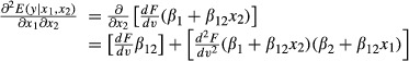
As Ai and Norton (2003) explain, in nonlinear models the cross-partial effect could be different from zero, even if β₁₂ = 0. To illustrate, if we again let v = β₀ + β₁x₁ + β₂x₂ + β₁₂(x₁ × x₂) and use the result from equation (5), we can write:

(6)

Even without an interaction term (β₁₂ = 0), the expression above for still has a nonzero value. Therefore, the statistical significance of the cross-partial derivative cannot be tested with a simple asymptotic z-statistic on β₁₂. Nor does the sign of β₁₂ necessarily indicate the sign of the cross-partial effect. Instead, the cross-partial effect must be evaluated for the specific nonlinear function in question. The extent to which the addition of an explicit interaction term changes either the marginal or cross-partial effects can be answered by comparing marginal effects from models with and without an explicit interaction term.

An additional feature of nonlinear models is the need to understand the distinction between the scale of interest and the scale of estimation. Some typical examples of the scale of interest in health services research include expenditures, and out-of-pocket costs in dollar amounts; utilization of health care services measured as inpatient, outpatient, emergency department visits, length of hospital stays; as well as probability of various outcomes such as any health care spending, any doctor visits, and indicators of unmet needs or other access to care measures. The scale of estimation, on the other hand, could be log transformation of the outcome variable when it is a continuous variable, or a nonlinear transformation of the probability that the outcome equals 1 (e.g., logit or probit of the probability) when the outcome is binary.

The appropriate choice of the scale of estimation is a critical decision in nonlinear modeling, because its misspecification could lead to biased results (Basu, Arondekar, and Rathouz 2006).

Extensions

Thus far, the information we have presented is contained in Ai and Norton (2003) and Norton, Wang, and Ai (2004). Next, we extend the basic model in several important directions. First, following Puhani (2008), we explain the interpretation of interaction effects in the special but common case of difference-in-differences (DD) models. Second, we extend the results to include other nonlinear variables in the model. Third, we discuss the odds ratio interpretation. Fourth, we explain how to interpret interaction terms in panel data models.

A Special Case: Difference-in-Differences Models

When subjects in a treatment group and a control group are observed in both the pretreatment and posttreatment periods and the pretreatment time trends in the outcome variable are not significantly different in the two groups, DD models can be used to estimate the effect of the treatment on the treated. One way to specify the model is by defining a variable Post that is equal to one if the observation is from the posttreatment period and zero if from the pretreatment period; and a variable Treat that is equal to one if the observation is from the treatment group and zero if from the control group.

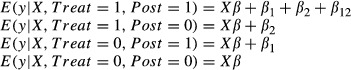
Letting the vector X represent some additional explanatory variables including a constant term, the linear DD model appears as follows:

(7)

Letting x denote the vector of covariates, the difference in E(y|x) from the pretreatment period to the posttreatment period for the treatment group is β₁ + β₁₂. The difference in E(y|x) from the pretreatment period to the posttreatment period for the control group is β₁, and thus, the difference in the differences in E(y|x) between the treatment and control groups from the pretreatment to the posttreatment periods is β₁₂. Thus, β₁₂ is an estimate of the treatment effect on the treated.

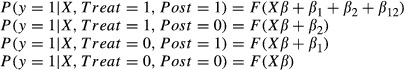
Again, using the logit or probit model as examples of nonlinear models, let the conditional probability that y = 1 be expressed as a function of the same linear index shown in equation (7): Xβ + β₁Post + β₂Treat + β₁₂(Post × Treat). We can write the nonlinear DD model as follows:

(8)

And the same DD logic can be applied:

The parameter β₁ allows the linear index (and hence the P(y = 1|x)) to be different for all subjects in the posttreatment period compared to the pretreatment period. β₂ allows the linear index (and hence the P(y = 1|x)) to be different for treatment subjects compared to control subjects. β₁₂ allows the linear index to be different in the posttreatment period and hence the conditional probability that P(y = 1|x) to be different over and above the difference attributable to the nonlinearity of the model for subjects in the treatment group versus the control group. It is the additional difference in the differences that provides a measure of the treatment effect on the treated.

Figures 3 and 4 show the effect of adding the explicit interaction term to a probit model. Figure 3 shows the relationships between the conditional probability that y = 1 and a continuous explanatory variable X in a model with no interaction term:

Figure 3.

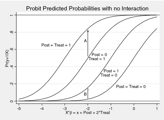
Nonlinear (Probit) Model without an Interaction Term

Figure 4.

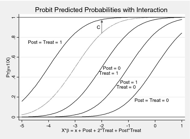
Nonlinear (Probit) Model with an Interaction Term (difference-in-differences)

(9)

The parameters β, β₁, and β₁₂ were set equal to 1, and β₂ was set equal to 2 (β₂ needs to be different than β₁ so that the lines do not lie on top of each other). In Figure 3, the curve furthest to the right corresponds to Post = 0, Treat = 0, thus to the cumulative distribution function of variable X which has a mean of zero. The curve to its left corresponds to Post = 1, Treat = 0. The third line from the right corresponds to Post = 0, Treat = 1. Finally, the curve furthest on the left corresponds to Post = 1, Treat = 1.

The DD estimate is the difference on vertical axis between the third and fourth lines from the right (distance A) versus the first and second lines from the right (distance B) evaluated at a specific value of the explanatory variables X. Figure 3 shows that in the absence of an explicit interaction term, distance A and distance B are not equal as they would be in a linear model and thus the nonlinear model will produce a nonzero DD estimate even without an interaction term. That is, the portion of the DD effect that Puhani (2008) noted should be held constant when evaluating the DD version of interactions in nonlinear models.

As shown in Figure 4, including the interaction term allows the curve furthest from the right, corresponding to Post = 1, Treat = 1, to shift even further to the left. That additional upward shift in the P (y = 1|x) from the dotted line to the solid line above it (distance C in Figure 4) is the portion of the DD effect attributable to the explicit interaction Post × Treat. In this special case that holds both Treat constant and Post constant but allows Post × Treat to vary, Puhani (2008) showed that the treatment effect on the treated is represented by the coefficient on the interaction term Post × Treat.

Nonlinear Models with Higher Powers of the Explanatory Variables

An additional source of nonlinearity arises when higher powers of explanatory variables (e.g., a squared term) are included in a nonlinear model. A squared term is an interaction between a continuous variable and itself, which is why this is of interest in this paper. In a logit or probit model, without other interaction terms or higher powers of the explanatory variables, the marginal effect of a variable x on the conditional probability that y = 1 has the same sign (though varying in magnitude) over the entire range of x, as shown as the slope of the dashed line in Figure 5 where the slope is always positive.

Figure 5.

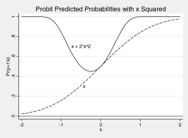
Predicted Probabilities with Squared Covariate

However, the inclusion of higher-order terms can produce relationships between x and y that require careful consideration. Consider the following model:

If the values of x are positive and the coefficients are positive, then the model including x² retains the relationship shown by the dotted line. However, if x extends into the negative range, the relationship between x and the conditional probability that y equals 1 is quite different from the usual S-shaped curve. Some examples of negative-valued covariates include de-meaned data (often age and age squared) to make the constant term more meaningful (Norton 1995; Norton et al. 2002), first-difference data indicating changes over time (French et al. 2010), two-stage residual inclusion (Terza, Basu, and Rathouz 2008; Van Houtven and Norton 2008), and standardized z-scores (Duflo 2000; Balsa et al. unpublished data). The addition of a squared term, shown by the solid line in Figure 5, causes P (y = 1|x) to become U-shaped (or possibly inverse U-shaped). As a result, there always will be some values of x (possibly out of sample) for which the full marginal effect is positive and some values for which it is negative.

Odds Ratios and Interactions

Some researchers prefer to explain results from logit models using the odds ratio interpretation instead of marginal effects, despite the well-documented confusion between risk ratios and odds ratios and the lack of policy meaning in an odds ratio (Lee 1994; Kleinman and Norton 2009). However, interaction terms make the odds ratio interpretation even more challenging (Norton, Wang, and Ai 2004). In a logit model without any interactions, the interpretation of a coefficient is the natural logarithm of the odds ratio. When an interaction term is included, the interpretation of its coefficient β₁₂ is more complicated. To see this, recall that in a simple logit model with an interaction term where x denotes the vector of covariates, the log odds are as follows:

(10)

Solving equation (10) for β₁₂ shows that it equals a complicated expression which is essentially the natural logarithm of the ratio of two odds ratios obtained by holding x₂ at 0 or 1 and incrementing x₁ by one unit (as shown in Appendix S1). This should further discourage the odds ratio interpretation.

Other Nonlinear Models

All of the results discussed so far are applicable to more complex nonlinear models, including ordered logit and probit models, multinomial logit and probit models, tobit models, count data models, and survival models, including event history and duration models. In each case, however, it is necessary to determine which of the three questions (additional explained variance, change in marginal effects, or change in cross-partial derivatives) one is interested in answering. Many computer programs will compute some form of marginal effects if requested, but the proper mathematical expressions for the cross-partial derivatives may have to be derived by the analyst using the formulas presented earlier in the paper as a guide.

Models for Panel Data

The interaction effect cannot be computed for a panel data logit model with fixed effects without further assumptions. Fixed effects logit models (also known as Chamberlain conditional logit models) are conditional on the sum of the dependent variable within each group. This sweeps out the group constant term (fixed effect). Without these group fixed effects (or additional assumptions), it is impossible to compute marginal effects of a single variable let alone a double (e.g., cross-partial) derivative or difference. For any model, it is impossible to predict the conditional expected value of the dependent variable without the constant term. The only direct interpretation of the coefficients in a fixed effects logit model is that of an odds ratio. Stata's margins command will make predictions after a fixed effects logit, but only by assuming that all the fixed effects are zero. In other words, after carefully modeling unobserved heterogeneity, the default is to make predictions assuming homogeneity. The same problem holds for random effects logit and random effects probit models.

Estimation

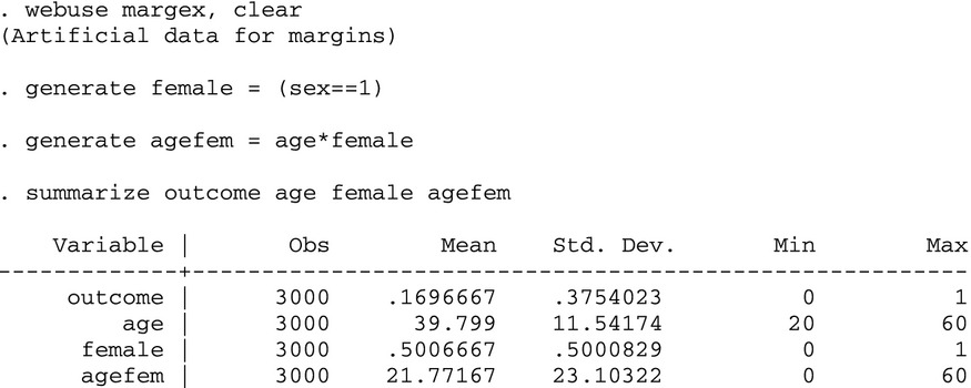
We next turn to the practical issue of how to answer the questions posed at the beginning of the paper when analyzing data. For this example, we use Stata's margex data set, which is fictitious data with a dichotomous outcome variable and various demographics. The margex data set has 3,000 observations. About 17 percent of observations have the outcome equal to one. Age ranges from 20 to 60, with a mean of 40. Half of the people in the sample are women (female = 1). The interaction between age and female (=age × female and denoted agefem) has a mean of 21.8 and ranges from zero to 60. We control only for age and female to keep the example simple.

Does the Interaction Term Improve the Goodness of Fit of the Model?

The question “Does the interaction term agefem improve the goodness of fit of the model” can be answered simply with a z-test on the coefficient of the interaction term in a logit model. The Stata 11 syntax uses c. to indicate a continuous variable, i. to indicate a dummy variable, and ## to include both main effects and all interactions. This syntax is necessary later for the margins command to understand the relationship between variables.

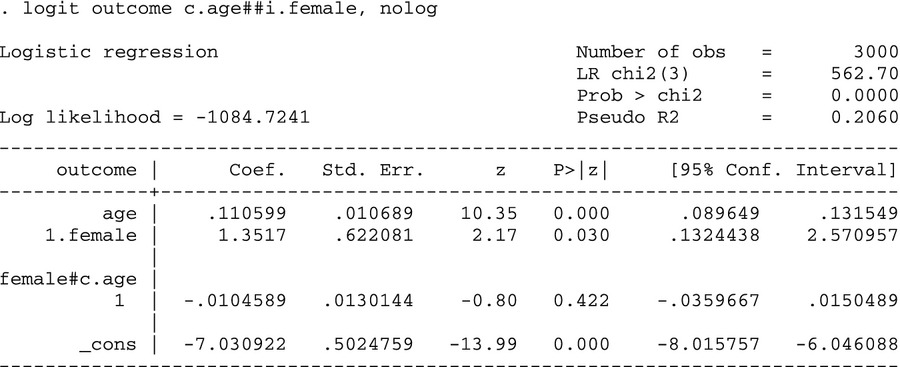The results show that the coefficients on age and female are positive and statistically significant, while the interaction coefficient is negative but not statistically significant. The z-statistic on the interaction term is −0.80, indicating that this variable does not explain much variation in the dependent variable.

Marginal Effects in Models with Interaction Terms

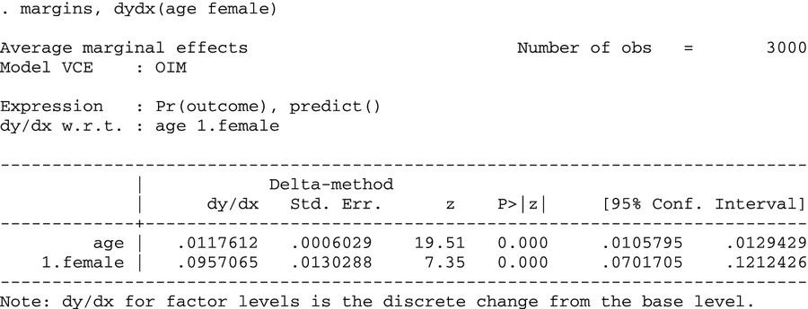
The question “What is the marginal effect of x₁ on the conditional expected value of y, when an interaction term is added to the model?” concerns marginal effects in models with interaction terms. The correct marginal effect of age and the incremental effect of gender can be found easily in Stata 11 with margins, as long as the logit command is run with the new syntax that highlights the relationship between the variables.

Using this syntax, Stata computes the correct marginal and incremental effects, taking into account the interaction term. The program computes the marginal effect for age using equation (A3a) in Appendix S1—the expression for the marginal effect of a continuous explanatory variable—with age and female set equal to their actual values for each observation. Then, the program computes the incremental effect for female using equation (A3b) in Appendix S1—the expression for the incremental effect of a discrete explanatory variable—with age set equal to its actual value for each observation and female alternating between 0 and 1. The results from equation (A3b) are averaged across all observations to obtain the average marginal effect of female. The standard error of the marginal effects is calculated at the means of the explanatory variables using the delta method (Greene 2008, pp. 68–70).1

Cross-Partial Derivatives in Models with Interaction Terms

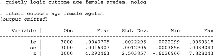
How does the marginal effect of age change when female change from 0 to 1? There are three basic ways to compute cross-partial derivatives in Stata: inteff, margins, and predictnl. First, we show the answer using inteff, a user-written command that works for logit and probit when there are exactly two variables interacted (Norton, Wang, and Ai 2004). The numeric calculations we present below can be enhanced by examining the interaction effects of two variables graphically. Greene (2010), for example, plotted how the partial effect of one variable (i.e., age) changes with that variable for different values of the second variable (i.e., female or male).

For the numeric calculation, we re-run the logit model using the original Stata syntax. The mean cross-partial derivative effect (labeled “ie”) is the average of the cross-partial derivative over all observations in the data set. For each observation, ie is the change in the conditional probability that outcome = 1 for a change in age as gender changes from zero to one. It is the difference in the marginal effect of age on the conditional probability that outcome = 1 between men and women. The mean interaction effect is positive—opposite in sign from the coefficient on the interaction term for most observations—and generally statistically significant. The average change in the predicted conditional probability that outcome = 1 for a 1-year increase in age differs between men and women by .41 percentage points, with women having higher marginal effects of age on average.

Although Stata's margins command can compute the derivative of only a single variable, we can manipulate the results to get the interaction effect by computing the derivative with respect to one variable at different values of the other variable. Again, if the interaction effect is the difference in the marginal effect of age on outcome between men and women, then one could compute the marginal effect of age for these two groups using the margins command and take the difference.

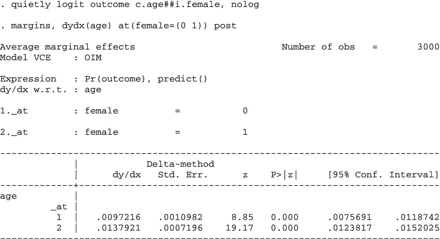The difference between .0137921 and .0097216 is exactly what we found before, namely .00407045. By symmetry, the same result could be approximated by computing the incremental effect of gender at different ages, and taking the difference. For example, one could do this for five pairs of ages (30 and 31, etc.). While none of the differences in the pairs is exactly .00407045, a weighted average would be close.

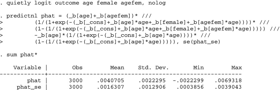
Finally, the general Stata command predictnl can be used for any nonlinear combination of the model's coefficients. Advantages include flexibility in use with any model or specification, and that it automatically computes the standard error. The difficulty in using this command is that it requires writing out the formula, and there is greater chance for a typo than either of the other methods. The formula in the predictnl command again corresponds to the idea of computing the marginal effect of age (derivative) for men and women, and then taking the difference. The formula is the difference in two derivatives, evaluated for men and for women. Again, we see that this method yields the same result that the full interaction effect in this simple model is about .0040705.

While the margins command is quite flexible, it cannot be used for every nonlinear model. For example, margins does not work for the log transformation (boxcox command).

Code for LIMDEP

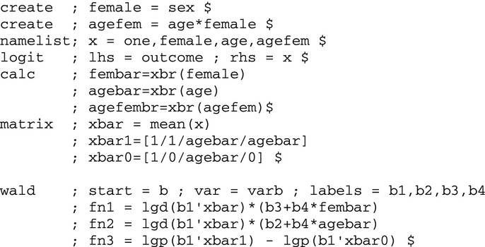
Having downloaded the margex data set and converted it to a LIMDEP systems file (using, e.g., StatTransfer), we can produce somewhat similar output with the following commands. (We are grateful to William Greene of New York University for providing the LIMDEP code.) The Wald command produces standard errors of the marginal effects taken at the means of the explanatory variables using the delta method.

Discussion

In this paper, we discussed reasons for including interaction terms in nonlinear models, as well as the proper interpretation of those terms. As Greene (2010) noted, the most important question to ask about models with interaction terms is “What meaning can be attached to the results?” This paper has dealt with both conceptual and computational aspects of interaction terms in nonlinear models, but that work needs to be preceded by development of a rigorous theoretical model to ensure correspondence between the empirical analysis and the hypotheses the analyst is trying to test.

SUPPORTING INFORMATION

Additional supporting information may be found in the online version of this article:

Appendix SA1: Author Matrix.

Appendix S1: Technical Appendix.

Please note: Wiley-Blackwell is not responsible for the content or functionality of any supporting materials supplied by the authors. Any queries (other than missing material) should be directed to the corresponding author for the article.

References

- Ai C, Norton EC. Interaction Terms in Logit and Probit Models. Economics Letters. 2003;80(1):123–9. [Google Scholar]
- Basu A, Arondekar BV, Rathouz PJ. Scale of Interest versus Scale of Estimation: Comparing Alternative Estimators for the Incremental Costs of a Comorbidity. Health Economics. 2006;15:1091–107. doi: 10.1002/hec.1099. [DOI] [PubMed] [Google Scholar]
- Duflo E. Child Health and Household Resources in South Africa: Evidence from the Old Age Pension Program. American Economic Review Papers and Proceedings. 2000;90(2):393–8. doi: 10.1257/aer.90.2.393. [DOI] [PubMed] [Google Scholar]
- French MT, Norton EC, Fang H, Maclean JC. Alcohol Consumption and Body Weight. Health Economics. 2010;19(7):814–32. doi: 10.1002/hec.1521. [DOI] [PMC free article] [PubMed] [Google Scholar]
- Greene WH. Econometric Analysis. 6th Edition. Upper Saddle River, NJ: Pearson Prentice Hall; 2008. [Google Scholar]
- Greene WH. Testing Hypotheses about Interaction Terms in non-Linear Models. Economic Letters. 2010;107(2):291–6. [Google Scholar]
- Kleinman LC, Norton EC. What's the Risk? A Simple Approach for Estimating Adjusted Risk Ratios from Nonlinear Models Including Logistic Regression. Health Services Research. 2009;44(1):288–302. doi: 10.1111/j.1475-6773.2008.00900.x. [DOI] [PMC free article] [PubMed] [Google Scholar]
- Lee J. Odds Ratio or Relative Risk for Cross-Sectional Data. International Journal of Epidemiology. 1994;23(1):201–3. doi: 10.1093/ije/23.1.201. [DOI] [PubMed] [Google Scholar]
- Norton EC. Elderly Assets, Medicaid Policy, and Spend-Down in Nursing Homes. Review of Income and Wealth. 1995;41(3):309–29. [Google Scholar]
- Norton EC, Wang H, Ai C. Computing Interaction Effects and Standard Errors in Logit and Probit Models. Stata Journal. 2004;4(2):154–67. [Google Scholar]
- Norton EC, Van Houtven CH, Lindrooth RC, Normand ST, Dickey B. Does Prospective Payment Reduce Inpatient Length of Stay? Health Economics. 2002;11(5):377–87. doi: 10.1002/hec.675. [DOI] [PubMed] [Google Scholar]
- Puhani PA. 2008. The Treatment Effect, the Cross Difference, and the Interaction Term in Non-Linear ‘Difference-in-Differences’ Models Discussion Paper Series: Forschungsinstitut zur Zukunft der Arbeit, Institute for the Study of Labor (April 2008) [accessed August 9, 2011]. Available at: http://ftp.iza.org/dp3478.pdf.
- Terza JV, Basu A, Rathouz PJ. Two-Stage Residual Inclusion Estimation: Addressing Endogeneity in Health Econometric Modeling. Journal of Health Economics. 2008;27(3):531–43. doi: 10.1016/j.jhealeco.2007.09.009. [DOI] [PMC free article] [PubMed] [Google Scholar]
- Van Houtven CH, Norton EC. Informal Care and Medicare Expenditures: Testing for Heterogeneous Treatment Effects. Journal of Health Economics. 2008;27(1):134–56. doi: 10.1016/j.jhealeco.2007.03.002. [DOI] [PubMed] [Google Scholar]
Associated Data
This section collects any data citations, data availability statements, or supplementary materials included in this article.