Compressive sensing based reconstruction in bioluminescence tomography improves image resolution and robustness to noise

Abstract

Bioluminescence Tomography attempts to quantify 3-dimensional luminophore distributions from surface measurements of the light distribution. The reconstruction problem is typically severely under-determined due to the number and location of measurements, but in certain cases the molecules or cells of interest form localised clusters, resulting in a distribution of luminophores that is spatially sparse. A Conjugate Gradient-based reconstruction algorithm using Compressive Sensing was designed to take advantage of this sparsity, using a multistage sparsity reduction approach to remove the need to choose sparsity weighting a priori. Numerical simulations were used to examine the effect of noise on reconstruction accuracy. Tomographic bioluminescence measurements of a Caliper XPM-2 Phantom Mouse were acquired and reconstructions from simulation and this experimental data show that Compressive Sensing-based reconstruction is superior to standard reconstruction techniques, particularly in the presence of noise.

1. Introduction

The insertion of genes coding for bioluminescent compounds allows the labelling of cells of interest such as cancerous cells. Such labelling typically provides a low output of bioluminescence photons but is specific, leading to very little background signal. Bioluminescent sources on the surface of a subject can be straightforwardly localised and quantified, but due to the optical scattering and absorption of tissue, the localisation and quantification of an internal bioluminescent source from surface measurements is non-trivial and it is necessary to perform Bioluminescence Tomography (BLT). BLT uses prior information about the optical properties of the subject to reconstruct the location and concentrations of internal bioluminescent sources from surface fluence measurements.

The tomographic reconstruction process requires that the propagation of bioluminescent light through tissue can be modelled. This can be accomplished through analytical and numerical methods [1]. If the image space (the spatial distribution of bioluminescence in the subject) is discretised into a number of finite and disjoint regions (analogous to pixels in a digital photograph) then the linearity of light propagation allows the propagation model to be formulated as a system of linear equations. This system can be expressed as Jx = y, where J is a matrix representing the physics of light propagation in tissue [2], x is a vector representing the bioluminescent source distribution (the image), and y is a vector representing the resulting light distribution (the surface measurements). The J matrix is commonly called a Jacobian or weight matrix, and is constructed from prior knowledge of the optical properties of the subject.

Given knowledge of y through measurement, and prior knowledge of J, it is necessary to reconstruct x. However, BLT problems are typically strongly underdetermined as a result of limitations on the number of measurements, and correlation between measurements. For example, in the experimental data examined in this paper it is necessary to reconstruct 10171 unknowns from 526 measurements.

Restrictions on the number of measurements arise primarily from the imaging setup which itself is limited by the duration for which a subject can be sedated, coupled with the typically low signal strength of bioluminescence which necessitates long measurement integration times. Strong correlations between measurements arise from the diffusive nature of light propagation in tissue and the practical constraint of taking measurements only on the surface of the subject. For these reasons, if more measurements are acquired at a particular wavelength, the set of measurements tends to become more correlated, limiting the benefit of increasing the number of measurements. In order to produce accurate images it is then necessary to develop and use reconstruction methods that are robust in the presence of this degree of non-uniqueness. Given small numbers of measurements in comparison to the number of unknowns, prior knowledge about BLT can help reduce the problem of non-uniqueness and so guide the reconstruction process. For example, BLT images the concentrations of bioluminescent chemicals in tissue. As concentrations are non-negative, constraining the unknowns to be non-negative halves the solution space in each dimension. In addition, BLT is commonly used in examinations of cancer growth, many of which grow in a fashion that preserves compactness of the bioluminescent tumour. The very low bioluminescence background in conjunction with the small size and compactness of the bioluminescent tumour result in a spatially sparse bioluminescence distribution, which can be used to further reduce the solution space.

Compressive Sensing (CS) allows the reconstruction of images that are sparse in a known representation given fewer measurements than unknowns [3], provided certain conditions on the measurements are satisfied [4,5]. It has the property of producing exact reconstruction with high probability, through maximisation of reconstruction sparsity whilst minimising measurement error. The measurement conditions require measurements to be:

• independent, so that each measurement provides unique information about the image.

• distributed, so that each measurement provides information about the entirety of the image.

If the set of measurements are sufficiently independent and distributed given the sparsity of the bioluminescence distribution being imaged, then there is a unique solution with maximum sparsity that matches the measurements, and that solution is the desired image. Sparsity maximisation can be used to extract the image from the measurements. In the case of BLT, the restriction of measurements to the subject surface and the diffusive nature of tissue limits the independence of measurements, and light absorption by tissue drastically reduces the sensitivity of measurements to bioluminescent sources deep within tissue. However, the large degree of sparsity possible in BLT images suggests that CS may nonetheless provide benefits over other reconstruction algorithms.

Standard reconstruction techniques attempt to solve Eq. (1):

$$\mathbf{x}=\underset{\mathbf{x}}{\text{min}}{\Vert \mathbf{y}-\mathbf{Jx}\Vert }_2^2$$ (1)

where ${\Vert \mathbf{x}\Vert }_p={\left({\sum }_{i=1}^N{\left|x_i\right|}^p\right)}^{\frac{1}{p}}$ is the L^p norm. In the case discussed here where the solution is expected to be spatially sparse, CS uses the insight that the most spatially sparse solution satisfying Eq. (1) is the exact solution with high probability (if the problem satisfies the necessary conditions [4, 5]). This is equivalent to finding a solution to ${\Vert \mathbf{y}-\mathbf{Jx}\Vert }_2^2=0$ that minimises the L¹ norm ||x||₁, which induces sparsity in the solution. The L⁰ norm, which essentially counts the number of non-zero components of x, induces sparsity even more strongly, but is a discontinuous function and so more difficult to minimise. In general, L^p norms for p ≤ 1 can be used to maximise sparsity.

Given the presence of noise in the measurements, minimizing the measurement error exactly is undesirable due to overfitting, and it becomes useful to consider L¹ minimization and measurement error minimization as objectives to be optimized jointly, with specified weights on each objective, as in Eq. (2):

$$\mathbf{x}=\underset{\mathbf{x}}{\text{min}}{\Vert \mathbf{y}-\mathbf{Jx}\Vert }_2^2+\lambda {\Vert \mathbf{x}\Vert }_1$$ (2)

where λ is a term that weights the sparsity constraint against the measurement error. It can be shown [6, 7] that Eq. (2) is equivalent to solving Eq. (3):

$$\mathbf{x}=\underset{\mathbf{x}}{\text{min}}{\Vert \mathbf{x}\Vert }_1\hspace{0.17em}\text{such}\hspace{0.17em}\text{that}\hspace{0.17em}{\Vert \mathbf{y}-\mathbf{Jx}\Vert }_2^2<\epsilon$$ (3)

where the measurement error threshold, ε, is some function of λ.

A number of CS-inspired reconstruction algorithms have been applied to BLT. Lu et al. [8] used a differentiable approximation of L¹ regularisation. He et al. [9] used an incomplete variables truncated Conjugate Gradient method, to solve sub-problems involving dynamic subsets of the problem unknowns, in conjunction with L¹ regularisation. Cong et al. [10] used a phase approximation simplification of the Radiative transport equation, permissable region approach and a constrained L¹ sparsity minimisation algorithm, with the constraint being a measure of the measurement discrepancy. Yu et al. [11] used L¹ regularisation. Gao et al. [12, 13] used the full Radiative Transport Equation, with both angularly-averaged and angularly-resolved data, in conjunction with both L¹ and Total Variation-based regularisation, to solve for sub-problems on meshes of different resolution and with an adaptive region of interest. The solution they proposed to choose the correct balance of L¹ and Total Variation weighting required additional prior knowledge of the bioluminescence distribution. He et al. [14] used an adaptive region of interest approach with L¹ regularisation. Liu et al. [15] used a dynamic quadratic approximation to the L^p norm, and explored how sensitive the reconstruction process is to the particular regularisation weight used. Zhang et al. [16] used a primal-dual interior-point approach, which does not need a regularisation weight, and employed an algorithm termination scheme which can be noise dependent. However, multiple termination criteria were used with the same termination threshold, and so its relationship to noise is non-trivial.

One issue not fully addressed in previous works [8, 9, 11–15] is that of choosing a regularisation/sparsity weighting, which is the subject of the presented work. Sparsity weighting is equivalent to the imposition of a measurement noise constraint, via the equivalence of Eq. (2) and Eq. (3). However, the mapping of sparsity weighting to a desired measurement noise measure (such as sum squared error) or vice versa is non-trivial. Sparsity weighting is also important when using regions of interest, as the sparsity of a given bioluminescence distribution is linked to the size and shape of the region of interest. As the region of interest shrinks around the non-zero parts of the bioluminescence distribution, the distribution necessarily becomes less sparse within the region of interest, and accordingly the sparsity weighting should be changed to account for this.

This work uses the iterative solution of a number of instances of Eq. (2), with decreasing sparsity weighting, to address this problem (section 2). Firstly, a measurement discrepancy termination threshold is given (based on the instrumental noise statistics). An initial sparsity weighting is generated that heavily favours the sparsity term. A solution to this problem is found, and then used as an initial solution to a new problem with slightly smaller sparsity weighting. This process repeats until the measurement discrepancy termination threshold is satisfied, or the measurement discrepancy term is heavily favoured over the sparsity term. This leads to one of two possible end states:

• The measurement discrepancy threshold is satisfied, and so the result is a local solution of Eq. (3).

• The measurement discrepancy term heavily outweighs the sparsity term, and so the result is a local solution of Eq. (1).

This process of solving a number of sub-problems using a previous solution as a starting point is similar to the approach used by Figueiredo et al. [6] to improve performance by “warm starting”.

This algorithm was tested against two other algorithms, using simulated and experimental measurements, and its performance quantitatively analysed (section 3).

2. Methods

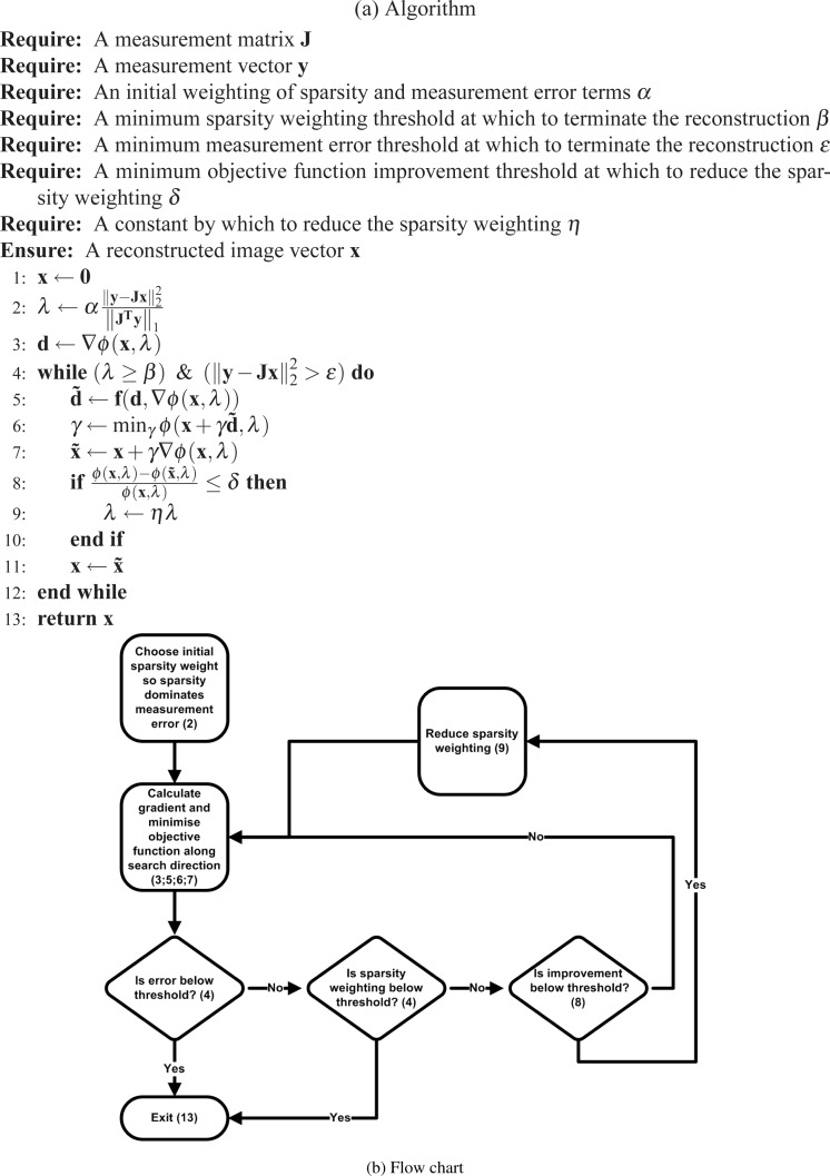
A Conjugate Gradient approach to solve Eq. (3) was implemented [7] (see Fig. 1), and shall be referred to as Compressive Sensing Conjugate Gradient (CSCG). A differentiable approximation of the L¹ norm in the form of Eq. (4) was used to simplify reconstruction:

$${\Vert \mathbf{x}\Vert }_1\approx \sum _i{\left(x_i^2+\mu \right)}^{\frac{1}{2}}$$ (4)

with the magnitude of μ insignificant relative to the magnitudes of non-zero x_i. The algorithm solves a number of sub problems for decreasing values of λ, using the solution to the previous sub problem as a prior for the next. As λ becomes small, the problem tends to Eq. (1), and so the solution produced by CSCG is also locally optimal in terms of measurement error. The initial value of λ is chosen as Eq. (5) so that the sparsity term is much larger than the measurement error term:

$${\lambda }_0={10}^5\frac{{\Vert \mathbf{y}\Vert }_2^2}{{\Vert {\mathbf{J}}^{\mathbf{T}}\mathbf{y}\Vert }_1}$$ (5)

The constant of 10⁵ was selected empirically to ensure that the sparsity term dominates the measurement error term. If the value is higher than necessary then the reconstruction result is unaffected, but the reconstruction time may display a small increase, as λ is decreased during the reconstruction. If the value is too low then the reconstruction process may be affected as the measurement error can reach the termination threshold before the solution is maximally sparsified. A set of sub-problems are then solved with decreasing λ until the measurement discrepancy condition is satisfied or λ satisfies inequality (6):

$${\lambda }_n\le \frac{{\lambda }_0}{{10}^{20}}$$ (6)

The value of 10²⁰ was also selected empirically to ensure that in the case where the measurement error threshold cannot be met, the reconstruction process does not terminate before it is reduced to solving Eq. (1). CSCG is also constrained to be non-negative, due to the physical non-negativity of luminophore distributions. This constraint is implemented via projection within the algorithm, where the projected solution x′ is calculated as Eq. (7).

$$x_i^{\prime }=\text{max}\left(x_i,0\right)$$ (7)

Fig. 1.

(a) CSCG algorithm pseudocode. ϕ(x, λ) is the objective function (see Eq. (2)). f is a vector function that generates a new search direction using the gradient of ϕ(x, λ) and the previous search direction. α was chosen in this work to be 10⁵. β was chosen in this work to be 10⁻²⁰ of the initial value of λ. η was chosen in this work to be 2^−1/2. (b) Flowchart of CSCG algorithm.

Two standard algorithms were used to provide a reconstruction performance comparison. These benchmark algorithms are Gauss-Newton (GN) and Non-negative Least Squares [17] (NNLS). The GN and NNLS algorithms have been implemented to solve Eq. (8):

$$\mathbf{x}=\underset{\mathbf{x}}{\text{min}}{\Vert \mathbf{y}-\mathbf{Jx}\Vert }_2^2+\alpha {\Vert \mathbf{Ix}\Vert }_2^2\hspace{0.17em}\text{such}\hspace{0.17em}\text{that}\hspace{0.17em}{x}_i\ge 0$$ (8)

which includes identity-matrix-based Tikhonov regularisation with regularisation weight α.

As GN is not non-negative, it is constrained to be non-negative via projection (see Eq. (7)). Unconstrained GN is a non-iterative algorithm, but the projection step necessitates an iterative approach, where the error introduced by projection is iteratively minimised via GN.

NNLS is intrinsically non-negative and so no modification is necessary to induce nonnegativity. Although NNLS solves the same equation as GN, it does so in a very different manner. A support set (initially consisting of one dimension) is defined such that the solution to the equation on this support set is non-negative, and the equation is solved on this support set. Dimensions are then iteratively chosen and added to the support set in a manner that preserves the non-negativity of the solution, until the equation is solved to the desired accuracy. Due to the use of a small and increasing support set this algorithm can be well suited to reconstructing sparse solutions, assuming that the algorithm chooses the correct support set.

Modeling of light transport in tissue was carried out using the NIRFAST software package [18], which solves the Diffusion Approximation to the Radiative Transport Equation through Finite Element Analysis.

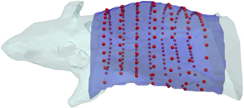
An XPM-2 Phantom Mouse (Caliper Life Sciences, Hopkinton, MA, USA) was imaged using a Computed Tomography (CT) and Fluorescence Tomography (FT) instrument at Dart-mouth College [19], which acquires data in rings around the circumference of the subject. A mesh of the mouse torso was created from CT data (see Fig. 2), and was used, in addition to the instrumental setup, in reconstructions involving both simulated or experimental measurements.

Fig. 2.

Caliper XPM-2 Phantom Mouse and the torso region used in reconstructions. The XPM-2 is shown in light blue, and the torso region used is overlaid in dark blue. The positions of the measurements acquired are shown as red spheres.

2.1. Simulation

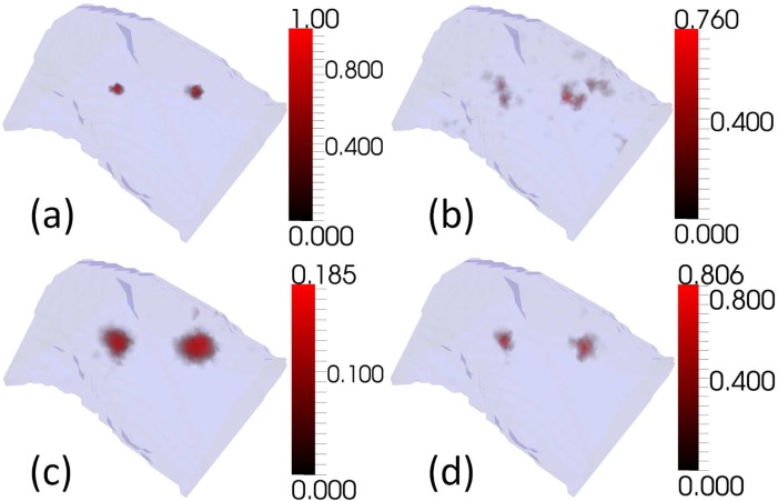
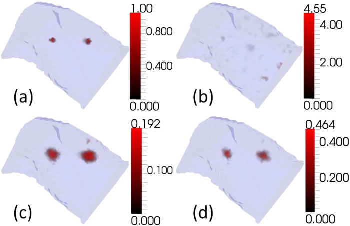
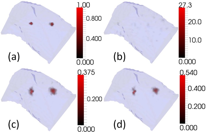
Simulations were conducted using the XPM-2 torso mesh with two embedded bioluminescent sources, and the measurement positions that were used in the imaging at Dartmouth College (see Fig. 2). The measurement process was simulated in the presence of normally distributed noise. Simulated measurements were calculated using a higher resolution version of the torso mesh than the one used for reconstruction. Five monochromatic wavelengths (560nm, 585nm, 602nm, 630nm, and 650nm) were used in simulations. Noise, where applied, was additive, drawn from a normal distribution with a mean of 0, and independently and identically distributed for each measurement. Three values of noise standard deviation were tested: 0%, 1% and 5% of the magnitude of the maximum simulated measurement (see Fig. 3, Fig. 4, and Fig. 5 respectively). For each noise level 30 samples of noise were generated and used. The noise threshold for CSCG (see ε in Fig. 1) was set to zero to be consistent with the experimental reconstruction, and measurements were removed to leave the same subset of measurements that was used in the experimental reconstruction (see section 2.2). A single regularisation weight for GN and NNLS of 10⁻⁵ was chosen empirically from simulations and used for all tests, as in practice one cannot know the best regularisation weight for data sets whose solution is unknown. The regularisation value was chosen to minimise regularisation whilst reducing artifacts at all noise levels.

Fig. 3.

Reconstructions of two bioluminescent sources using simulated measurements in the absence of measurement noise. (a)Target (b)GN (c)NNLS (d)CSCG

Fig. 4.

Reconstructions of two bioluminescent sources using simulated measurements, as Fig. 3, in the presence of 1% normally distributed noise.

Fig. 5.

Reconstructions of two bioluminescent sources using simulated measurements, as Fig. 3, in the presence of 5% normally distributed noise.

2.2. Experiment

Measurements of the XPM-2 Phantom Mouse were acquired using the instrument at Dartmouth college, from five light bands centred around 560nm, 585nm, 602nm, 630nm, and 650nm, with widths of 10nm, resulting in 1120 measurements. The measurement noise statistics were unknown and so the noise threshold for CSCG (see ε in Fig. 1) was set to zero. As the quantity being measured is the number of photons arriving at the detectors, all measurements should be positive. However, due to instrumental error some measurements were negative. The maximum negativity of measurements was used to estimate which measurements were noise dominated. All measurements with magnitudes less than five times the absolute value of the most negative measurement were considered noise-dominated and removed, leaving a total of 526 measurements from which to reconstruct 10171 unknowns.

3. Results and discussion

Examples of simulated reconstructions (see Fig. 3, Fig. 4, and Fig. 5) show qualitatively that CSCG reconstructs well, and with reduced noise artifacts at all noise levels compared to GN and NNLS. Figure 3 shows reconstructions in the absence of noise. None of the algorithms succeed in reconstructing the target sources exactly. This is to be expected as modelling error was introduced by reconstructing from the measurements using a coarser mesh than was used to generate them. It is not possible for the coarser mesh to represent the target sources exactly. GN reconstructs the sources, but with much noise. This could potentially be reduced by increasing the regularisation weight. NNLS reconstructs with little noise, although more than CSCG, but with significant source broadening. This could potentially be reduced by decreasing the regularisation weight. As noise of 1% and 5% is added in Fig. 4 and Fig. 5 respectively, it can be seen that the performance of all algorithms degrades as the level of noise increases. GN shows the greatest level of degradation, with image artifacts dominating the target sources at both noise levels. At 1% noise, both NNLS and CSCG are visually very similar to the noiseless case, although the maximum intensity of the CSCG reconstruction drops significantly. At 5% noise both NNLS and CSCG show significant changes in reconstruction quality in terms of source localisation and size, although NNLS displays greater change.

Examining reconstruction performance quantitatively, Table 1 shows that CSCG displays superior localisation performance to both GN and NNLS, with localisation better or equal to the other algorithms at all noise levels and for both sources, with a maximum localisation error of 1.7mm. GN shows markedly inferior localisation performance to the other two algorithms at all noise levels and for both sources, with a maximum localisation error of 5.3mm. NNLS shows similar performance for source A, but consistently inferior performance for source B, with a maximum localisation error of 1.7mm as compared to 1.1 mm for CSCG. Reconstruction quality for both NNLS and CSCG is broadly similar, and degrades as noise increases, but both algorithms achieve localisation on average within 2mm of the true location.

Table 1.

Simulation localisation error (mm) of mean reconstructed source centre. Source locations were calculated by taking the centres of fitted Gaussian distributions. Source A is the left-most source, and source B is the right-most source, as displayed in Fig. 3, Fig. 4, and Fig. 5. At each noise level, 30 samples of noisy measurements were generated. The location of each source was taken to be the location of the maximum value in a region (a sphere of radius 8mm) around the true source centre.

Noise	Source A			Source B
	GN	NNLS	CSCG	GN	NNLS	CSCG
0%	1.8	0.6	0.6	3.6	1.6	0.9
1%	4.0	1.0	0.5	2.9	0.9	0.7
5%	5.3	1.7	1.7	2.8	1.7	1.1

Table 2 gives the reconstructed source size, and the trend here is consistent with the qualitative observations. Here NNLS performance is inferior in all tests except for 5% noise and source A, with a minimum volume of 82% of the true volume, and a maximum volume of 740%, and displays great variation as the level of noise changes. GN uniformly underestimates the size of the sources, with a minimum volume of 43% of the true volume, and a maximum volume of 86%, but given the poor localisation performance the volumes given may be those of image artifacts. CSCG reconstructs both sources well and shows the greatest resilience to noise, with a minimum volume of 57% of the true volume, and a maximum volume of 230%. It is possible that the performance of GN and NNLS could be improved by tuning the regularisation parameters for each instance of noise separately, but this is not practical in an experimental situation as one does not know the true image. No hyperparameters of CSCG were changed before any of the reconstructions at any noise level, indicating that CSCG performs well and is robust to noise.

Table 2.

Simulation mean volume (mm³) (see Table 1) as a percentage of the true volume. The volume of each source was taken to be the connected volume enclosed by half the maximum value in the region, containing the location of the maximum value.

Noise	Source A			Source B
	GN	NNLS	CSCG	GN	NNLS	CSCG
0%	43%	340%	74%	86%	740%	96%
1%	36%	290%	110%	72%	660%	150%
5%	26%	82%	57%	58%	330%	230%

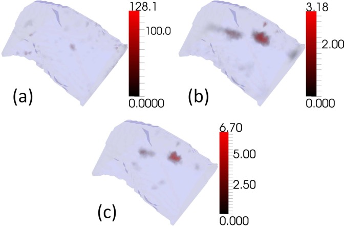
The reconstruction performance of the three algorithms in an experimental situation can be found in Fig. 6. The locations and sizes of two sources in the XPM-2 Phantom Mouse are unfortunately not known sufficiently precisely to the authors to allow a quantitative analysis, but qualitatively CSCG is again superior. The CSCG reconstruction displays improved source compactness and reduced noise artifacts compared to GN and NNLS. GN fails to reconstruct either source. The reconstructions display significantly different intensities for the two sources, which may result from measurement artifacts or inadequate prior knowledge of the optical properties of the phantom material.

Fig. 6.

Reconstructions of experimental measurements of an XPM-2 Phantom Mouse (Caliper Life Sciences, Hopkinton, MA, USA). (a)GN (b)NNLS (c)CSCG

4. Conclusion

CSCG demonstrates increased robustness to noise in comparison to GN and NNLS in both simulation and experiment, in terms of reduced noise artifacts and consistent reconstructed values across different levels of noise. The multi-level reconstruction of CSCG removes the need to empirically select regularisation values whilst still providing good quality reconstructions, which makes the reconstruction process more objective. However, CSCG does not necessarily converge on a global minimum, and is not optimised for efficiency, which are two areas for possible improvement.

CS improves reconstruction quality, and allows robust reconstruction from minimal data sets. Whether, and in what circumstances, BLT measurements are sufficient to allow true CS reconstruction is an open question. By design of instrumentation and measurement schemes to better satisfy the CS conditions, such as through optimisation of measurement location and wavelength, superior reconstruction fidelity is achievable.