Symmetries in geology and geophysics

Abstract

Symmetries have played an important role in a variety of problems in geology and geophysics. A large fraction of studies in mineralogy are devoted to the symmetry properties of crystals. In this paper, however, the emphasis will be on scale-invariant (fractal) symmetries. The earth’s topography is an example of both statistically self-similar and self-affine fractals. Landforms are also associated with drainage networks, which are statistical fractal trees. A universal feature of drainage networks and other growth networks is side branching. Deterministic space-filling networks with side-branching symmetries are illustrated. It is shown that naturally occurring drainage networks have symmetries similar to diffusion-limited aggregation clusters.

Symmetries appear in a wide variety of contexts in geology and geophysics. Rocks are made up of minerals and the symmetry aspects of minerals constitute a major part of any course in mineralogy. Many advances in x-ray diffraction were motivated by studies of minerals. The symmetries of crystalline structures are generally associated with translations, rotations, and reflections. In this paper, however, we will focus our attention on a fourth symmetry: scale invariance. Scale invariance is generally associated with fractals and self-similarity. The classic example is the Cantor set, illustrated in Fig. 1. At each order, the remaining line segments are divided into three parts and two are retained. The fractal dimension is D = log(N₂/N₁)/log(r₁/r₂), where N is number and r is length for the Cantor set D = log2/log3 = 0.6309, intermediate between the Euclidean dimension of a line (D = 1) and a point (D = 0).

Figure 1.

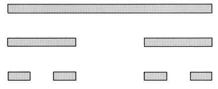
Illustration of the Cantor set; the line segment at zero order is divided into three equal parts and two are retained. The two line segments at first order are each divided into three equal parts and two are retained at second order. This is a fractal construction with fractal dimensions D = log2/log3 = 0.6309. This is an example of scale-invariant symmetry.

It should be remembered that Mandelbrot (1) introduced the concept of fractals in terms of the length of a rocky coastline. The length of a rocky coastline scales with the length of the measuring rod used as a fractional inverse power (2). This is a statistical symmetry rather than a deterministic symmetry. An illustration of this is given in Fig. 2. On the left is a third-order Koch triadic island. This is a deterministic fractal with D = log4/log3 = 1.262, intermediate between the Euclidean dimension of an area (D = 2) and a line (D = 1). On the right is the map of an actual island, Dear Island, Maine. Using either the measuring-rod method or the box-counting method (2), this island satisfies fractal statistics to a good approximation, with D ≈ 1.4. Rocky coastlines generally exhibit statistical scale-invariant symmetries. Other examples of scale-invariant symmetries in geology and geophysics include fragments, faults, earthquakes, ore deposits, oil fields, and volcanic eruptions. The fractal dimension associated with a scale-invariant symmetry is a quantitative measure of texture; increased fractal dimensions correspond to increased roughness.

Figure 2.

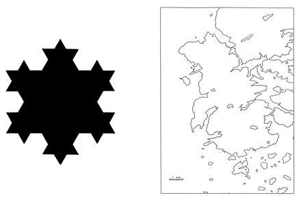
Island constructions exhibiting deterministic and statistical scale-invariant symmetries. (Left) The deterministic third-order Koch triadic island. This is another fractal construction with fractal dimension D = log4/log3 = 1.262. (Right) A map of Dear Island, Maine. The rocky coastline of this island exhibits a statistical scale-invariant symmetry; the fractal dimension is D ≈ 1.4.

Self-similar symmetries can also be associated with self-affine fractals; some statistically self-similar time series are examples of self-affine fractals. A deterministic, self-affine fractal is illustrated in Fig. 3. The vertical scale is arbitrary relative to the horizontal scale, thus the self-affine terminology. At first order, the width r_o is divided in four parts and the height h_o is divided into two parts, and the generator for the fractal construction is illustrated in Fig. 3b. At second order, as illustrated in Fig. 3c, each first-order, straight-line segment in Fig. 3b has been replaced by the rescaled generator. The construction is continued to third order in Fig. 3d. This construction is a deterministic example of a “random” walk in that y/h_o = (x/r_o)½. Using rectangular boxes with dimensions h_o/n and r_o/n, n = 1, 2, 3, … , the box-counting fractal dimension of this construction is D = 1.5.

Figure 3.

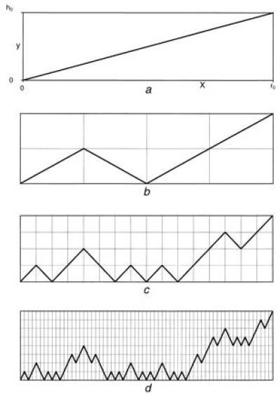
Illustration of a deterministic self-affine fractal. (a) At zero order, a rectangular region of width r_o and height h_o is considered. (b) The first-order fractal, which is also the generator. (c) Each straight-line segment in b is replaced by a scaled generator to give the second-order fractal. (d) Each straight-line segment in c is replaced by a scaled generator to give a third-order fractal.

Fractional Brownian walks are examples of statistical self-affine fractals. Examples of both fractional Gaussian noises (a) and fractional Brownian walks (b) are given in Fig. 4. In all cases, the power spectral density S is related to the frequency f by the relation S ∝ f^−β (an equivalent relation is A_n ∼ f_n^−β/2, where A_n is the Fourier coefficient corresponding to the frequency f_n). The example given in Fig. 4a for β = 0 is a Gaussian white noise. A random value is chosen from a Gaussian distribution at each time step; adjacent values are uncorrelated.

Figure 4.

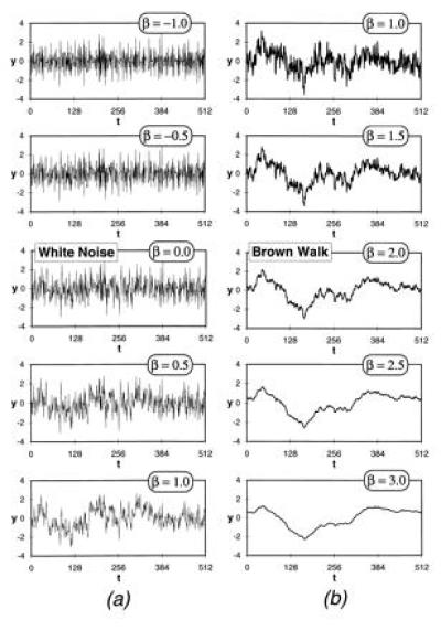
(a) The white Gaussian noise β = 0, has been filtered to give fractional Gaussian noises with β = −1.0, −0.5, 0.5, and 1.0. (b) Each of these noises has been summed to give fractional Brownian walks. The walks are self-affine fractals.

The fractional Gaussian noises given in Fig. 4a have been obtained using a standard filtering technique. The Fourier coefficients of the white noise have been increased or decreased to give the appropriate β and the resulting Fourier series inverted to give the fractional Gaussian noise. For β = 0.5 and 1.0, adjacent values became correlated, since the high frequency noise has been filtered out. For β = −0.5 and −1.0, adjacent values become anticorrelated.

A Brownian walk is the running sum of a Gaussian white noise. The Gaussian white noise in Fig. 4a (β = 0) has been summed to give the Brownian walk in Fig. 4b (β = 2). Each of the fractional Gaussian noises in Fig. 4a has been summed to give the fractional Brownian walks in Fig. 4b. The β of the summed fractional Brownian walk β_fw is related to the β of the fractional Gaussian noise β_fn by β_fw = β_fn + 2. A Gaussian white noise has a flat spectrum so that β_wn = 0, thus the Brownian walk has β_βw = 2. The fractal dimension of a fractional Brownian walk obtained by box counting is related to β_fw by D = (5 − β_fw)/2. Thus the fractal dimension of a Brownian walk (β = 2) is D = 1.5, the same fractal dimension as the deterministic fractal illustrated in Fig. 3. Fractional Brownian walks with 1 < β_fw < 3 are self-affine fractals with 2 > D > 1.

There are many examples of self-similar time series in geology and geophysics. One is the height of topography along a linear track; to a good approximation, the height of topography is a Brownian walk. Thus, if you walk a distance x in a straight line, your mean change in elevation Δh will be given by Δh = cx½, where the constant c depends on the roughness of the local terrain. The temporal variations of the earth’s magnetic field and the spatial variations of the earth’s gravity field have also been modeled as self-affine time series.

Self-Similar Networks

We now turn our attention to fractal trees and growth networks. Drainage networks are a classic example of statistical fractal trees. A small example is illustrated in Fig. 5a. The 100-m scale is shown, because without the specified scale it would be impossible to tell whether the drainage network covered 1 km or 1000 km.

Figure 5.

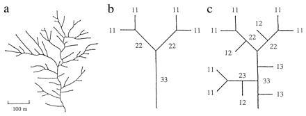
(a) Example of a fourth-order drainage network. (b) Binary self-similar fractal tree. (c) Binary self-similar fractal tree with side branches.

An example of a binary deterministic fractal tree is given in Fig. 5b. This is a highly ordered structure in which the single stem bifurcates into two branches, each with one-half the length of the stem. These two branches in turn bifurcate to form four branches, each with one-quarter the length of the stem. Obviously this construction could be carried to higher and higher orders.

However, a major difference between this binary tree and the drainage network is the absence of side branching. Branches that terminate originate from branches of all orders. A fractal tree with side branching is given in Fig. 5c. To quantify fractal trees, it is necessary to introduce a stream ordering system. In the Strahler (3) system for drainage networks, a stream with no upstream tributaries is a first-order (i = 1) stream. When two first-order streams combine, they form a second-order (i = 2) stream; when two second-order streams combine, they form a third-order (i = 3) stream; and so forth. The total number of ith order streams is N_i and their mean length is r_i. Tokunaga (4) modified the Strahler system to include side branching. A first-order branch joining another first-order branch is denoted 11 and the number of such branches is N₁₁; a first-order branch joining a second-order branch is denoted 12 and the number of such branches is N₁₂; a second-order branch joining a second-order branch is denoted 22 and the number of such branches is N₂₂; and so forth. This classification of branches is illustrated in Fig. 5.

The branch numbers N_ij, i ≤ j, constitute a square, upper triangular matrix. This formulation is illustrated in Fig. 6a. The branch-number matrices for the drainage network and deterministic fractals illustrated in Fig. 5 a–c are given in Fig. 6 b–d. The total number of streams of order i, N_i, is related to the N_ij by:

1

for a fractal tree of order n as illustrated in Fig. 6.

Figure 6.

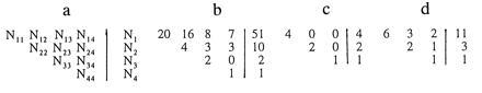
(a) Illustration of the branch-number matrix. (b–d) Branch number matrices for the fractal trees illustrated in Fig. 5 a–c.

Horton (5) defined the bifurcation ratio R_b according to:

2

He also introduced the length-order ratio:

3

Empirically it was recognized that both R_b and R_r are nearly constant for a range of stream orders in all drainage basins, and this observation constitutes two of Horton’s laws. The fractal dimension D of a drainage basin can be expressed in terms of the bifurcation and length-order ratios according to:

4

Thus the validity of Horton’s laws implies drainage networks are fractal trees.

The deterministic fractal tree illustrated in Fig. 5b has R_b = 2 and R_r = 2 so that D = 1, from Eq. 4. The deterministic fractal illustrated in Fig. 5c has R_r = 2 but R_b is not constant. However, it is easy to show that R_b → 4 for large i. Thus from Eq. 4D → 2 for large i.

Tokunaga (4) found that a broader classification of the symmetries of drainage basins could be expressed in terms of branching ratios T_ij. These are the average number of branches of order i joining branches of order j, i < j. Branching ratios are related to branch numbers by:

5

Again the branching ratios T_ij constitute a square, upper triangular matrix, as illustrated in Fig. 7a. The branching ratio matrices for the drainage network and deterministic fractals illustrated in Fig. 5 a–c are given in Fig. 7 b–d.

Figure 7.

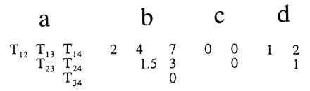
(a) Illustration of the branching-ratio matrix. (b–d) Branching-ratio matrices for the fractal trees illustrated in Fig. 5 a–c.

Peckham (6) has determined the branching-ratio matrices for the Kentucky River basin in Kentucky and the Powder River basin in Wyoming, and his results are given in Fig. 8. Both river basins are eighth order, with the Kentucky River basin having an area of 13,500 km² and the Powder River basin an area of 20,181 km². For the Kentucky River basin, the bifurcation ratio is R_b = 4.6, the length-order ratio is R_r = 2.5, and the fractal dimension from Eq. 4 is D = 1.67; for the Powder River basin the bifurcation ratio is R_b = 4.7, the length-order ratio is R_r = 2.4, and the fractal dimension from Eq. 4 is D = 1.77.

Figure 8.

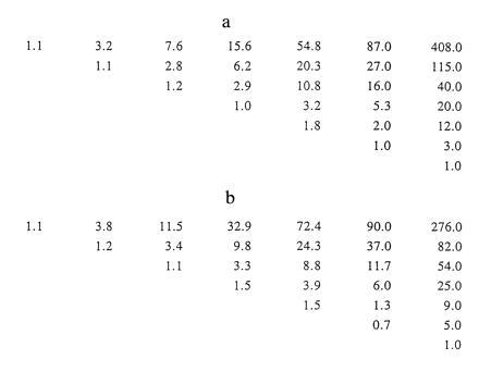
Branching-ratio matrices for (a) the Kentucky River basin and (b) the Powder River basin, as obtained by Peckham (6).

Tokunaga (4) defined a more restrictive class of fractal trees by requiring T_i,i+k = T_k, where T_k is a branching ratio that depends only on k = j − i. It is seen from Fig. 7d that the deterministic side branching network illustrated in Fig. 5c satisfies this condition with T₁₂ = T₂₃ = T₁ = 1. The condition is also satisfied if the construction is extended to higher orders. The Tokunaga condition is seen to be approximately valid for the drainage networks considered in Fig. 8.

Tokunaga (4) introduced a more restricted class of self-similar side-branching trees by requiring for self-similarity of side-branching that:

6

This is now a two-parameter family of trees. For the fractal tree illustrated in Fig. 5c, we have a = 1 and c = 2. Both the results for the Kentucky River basin and the Powder River basin correlate well with Eq. 6, taking a = 1.2 and c = 2.5.

As discussed above, the deterministic fractal illustrated in Fig. 5c becomes space filling (D → 2) for large order. Another fractal construction that becomes space filling in two dimensions (D → 2) for large order is illustrated in Fig. 9. The large circle in Fig. 9a is the original (O-order) node (bud) and three branches (line segments) emanate from it. The small circles are first-order nodes (buds) and there are two types, three exterior nodes and a single interior node. The interior node bisects the interior branch; the nodes are equally spaced. In Fig. 9b, three tip branches (line segments) emanate from each tip node and two side branches (line segments) emanate from the interior node. Eleven tip nodes and five interior nodes are introduced at this order. The construction is continued in Fig. 9 c and d. The length-order ratio for the construction is R_r = 2.

Figure 9.

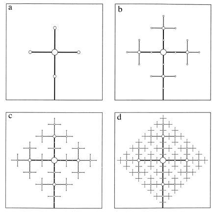
An illustration of an area-filling Tokunaga fractal tree. The generator for this fractal tree is illustrated in (a). Three tip branches emanate from the central node. Three exterior nodes are placed at the tips and an internal node bisects the internal branch. In b, nine tip branches emanate from the tip nodes and two side branches emanate from the internal node. Eleven exterior nodes are placed at the tips and five internal nodes bisect the internal line segments. The construction is continued in c and d. The length-order ratio for the construction is 2.

The branch-number and branch-ratio matrices for this construction are given in Fig. 10 a and c. The branching ratios for arbitrary order are given by:

7

The construction is a Tokunaga fractal tree. The branch numbers and bifurcation ratios are given in Fig. 10b. Again, for large order trees, R_b becomes independent of order and for this case R_b → 4; thus D → 2 and the construction becomes space filling.

Figure 10.

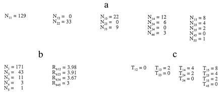
(a) Branch-number matrix for the Tokunaga tree illustrated in Fig. 9. (b) Branch numbers and bifurcation ratios. The bifurcation ratio approaches 4 (D → 2) for high orders. (c) Branch-ratio matrix for the tree.

In Fig. 11, the space-filling tree given is Fig. 9 is used to construct a hierarchy of synthetic drainage networks that drain a square island. The drainage basin boundaries are illustrated by dashed lines. There are clearly many symmetries in this construction. For actual drainage basins the area-order ratio R_A is defined as:

8

where A_i is the drainage area of a basin of order i. Horton (5) has shown that R_A is generally a constant in a region independent of order, with a typical value being R_A = 5. For the networks illustrated in Fig. 11 we have R_A = 4.

Figure 11.

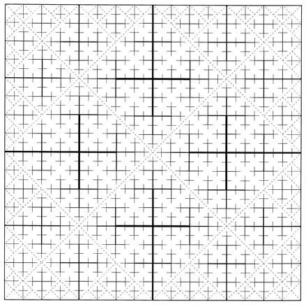
The synthetic drainage network illustrated in Fig. 9 is used to construct a hierarchy of networks that drain a square island. The divides between drainage networks are illustrated by dashed lines. The orders of the drainage networks are 2, 3, 4, and 5. The area-order ratio is R_A = 4.

The discussion given above has been restricted to the two-dimensional platform of drainage networks. To develop a full understanding of how drainage networks are related to erosion, it is necessary to include topography. Again, this can be done using empirical symmetries obtained for drainage basins. The slope-order ratio R_s is defined by:

9

where α_i is the slope of a stream of order i. Horton (5) also found that R_s is also constant in a drainage basin independent of order, with a typical value being R_s = 1.8.

Taking R_s = 2, synthetic topography has been constructed from the synthetic drainage basins illustrated in Fig. 11; the result is given in Fig. 12a. Clearly this synthetic topography is much more deterministic than typical topography; however, the drainage network on the Wasatch front near Mapleton, UT, illustrated in Fig. 12b certainly resembles the synthetic system.

Figure 12.

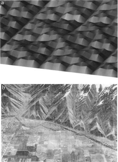
(a) Synthetic topography based on the synthetic drainage network given in Fig. 11. (b) Photograph of the drainage network on the Wasatch Front near Mapleton, UT (7).

A space-filling fractal network can also be constructed in three dimensions. An example is given in Fig. 13. The construction is on a body-centered cubic lattice. Eight branches emanate from a central node. First-order nodes are placed at the tips of these branches and seven tip branches emanate from each exterior nodes. At the next order, Fig. 5b, exterior nodes are placed at the tips and eight internal nodes bisect the internal branches. At the next order, seven tip branches would emanate from each of the tip nodes and six branches from each of the internal nodes. The length-order ratio for the construction is 2.

Figure 13.

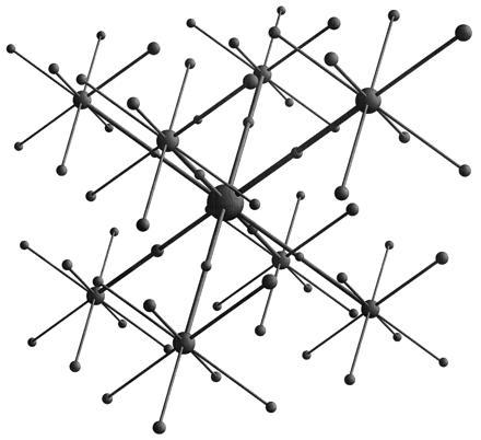
An illustration of a volume-filling Tokunaga fractal tree. The construction is based on a body-centered cubic lattice. The large node at the center of the cube emits eight tip branches to the corners of a cube. The eight smaller nodes at the tips of these branches each emit seven tip branches. Fifty-six exterior nodes are placed at the tips of these branches and eight internal nodes bisect the internal branches. At the next order, each tip node would emit seven tip branches and each internal node would emit six tip branches. The length-order ratio is 2.

The branch-number and branch-ratio matrices for this construction are given in Fig. 14 a and c. The branching ratios for arbitrary are given by:

10

Again the construction is a Tokunaga fractal tree. The branch numbers and bifurcation ratios are given in Fig. 14b. For large-order trees, R_b → 8 so that D → 3, and the construction becomes volume filling.

Figure 14.

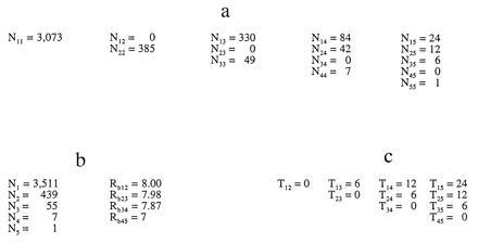
(a) Branch-number matrix for the Tokunaga tree illustrated in Fig. 13. (b) Branch numbers and bifurcation ratios. The bifurcation ratio approaches 8 (D → 3) for high orders. (c) Branch-ratio matrix for the tree.

Tokunaga branching statistics provide an excellent basis for analyzing the taxonomy of networks and trees. However, it does not provide any information on how the networks form. One approach to the generation of statistical branching networks is diffusion-limited aggregation (DLA).

DLA

The concept of DLA was introduced by Witten and Sander (8). They considered a grid of points on a two-dimensional lattice and placed a seed partice near the center of the grid. An accreting particle was randomly introduced on a “launching” circle and was allowed to follow a random path until: (i) it accreted to the growing cluster of particles by entering a grid point adjacent to the cluster, or (ii) until it wandered across a larger “killing” circle.

Ossadnik (9) has considered the branching statistics of 47 off-lattice DLA clusters, each with 10⁶ particles; a typical example is illustrated in Fig. 15. The sparse dendritic structure results because particles are more likely to accrete near the tips of the cluster rather than the deep interior. The networks were typically found to be 11th order. The average bifurcation ratio for the clusters was found to R_b = 5.15 ± 0.05 and the average length-order ratio R_r = 2.86 ± 0.05, and from Eq. 4, the corresponding fractal dimension is D = 1.56.

Figure 15.

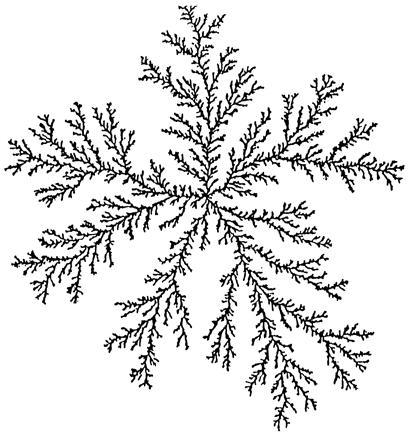
A two-dimensional, off-lattice DLA cluster with 10⁶ particules (9).

To analyze the branching statistics of DLA clusters, Ossadnik (9) used the ramification matrix introduced for DLA by Vannimenus and Viennot (10). In terms of the branching ratios T_ij, the terms of the ramification matrix are defined by:

11

The terms of the ramifications matrix obtained for DLA by Ossadnik are given in Fig. 16. For a Tokunaga self-similar fractal tree for which (Eq. 6) is valid, the terms of the ramification matrix are given by:

12

For large values of j, this becomes:

13

Taking c = 2.7, this relation is compared with the DLA data given in Fig. 16. It is seen that the DLA clusters are Tokunaga self-similar fractal trees to a good approximation.

Figure 16.

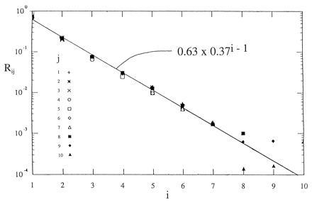
Dependence of the terms of the ramification matrix R_ij for the branching statistics of a DLA cluster on the branch order i for various branch orders j. Branches of order i join branches of order j, so that i < j. The data points are for an average of 47 off-lattice DLA clusters, each with 10⁶ particles (9). The straight-line correlation is with the Tokunaga relation (Eq. 13), taking c = 2.7.

Conclusions

One of the most important symmetries in geology and geophysics is scale invariance. In general, this symmetry is statistical rather than deterministic, is only approximate, and extends over only a finite range of scales. Landforms are a prime example of this symmetry. The length of coastlines or topographic contours are classic examples of self-similar fractals. Topography along a linear track is a classic example of a self-affine fractal. Both exhibit power-law scaling.

A ubiquitous feature of landforms on the Earth are drainage networks. These also exhibit scale-invariant symmetries and are recognized as fractal trees. Power-law scaling for fractal trees include the bifurcation ratio, the length-order ratio, the area-order ratio, and the slope-order ratio. A more complete taxonomy of drainage networks (and other networks) involves the statistics of side branching. Tokunaga (4) proposed a self-similarity of side branching applicable to symmetric deterministic trees, actual drainage networks, and DLA clusters. This taxonomy should be applicable to a wide range of growth networks in biology and other fields.

References

- 1.Mandelbrot B. Science. 1967;156:636–638. doi: 10.1126/science.156.3775.636. [DOI] [PubMed] [Google Scholar]
- 2.Turcotte D L. Fractals and Chaos in Geology and Geophysics. Cambridge, U.K.: Cambridge Univ. Press; 1992. [Google Scholar]
- 3.Strahler A N. Trans Am Geophys Union. 1957;38:913–920. [Google Scholar]
- 4.Tokunaga E. Japan Geomorphology Union. 1984;5:71–77. [Google Scholar]
- 5.Horton R E. Geol Soc Am Bull. 1945;56:275–370. [Google Scholar]
- 6.Peckham S D. Water Resour Res. 1995;31:1023–1029. [Google Scholar]
- 7.Gori, P. I., ed. (1993) U.S. Geol. Survey Professional Paper, Publ. No. 1519.
- 8.Witten T A, Sander L M. Phys Rev Lett. 1981;47:1400–1403. [Google Scholar]
- 9.Ossadnik P. Phys Rev A At Mol Opt Phys. 1992;45:1058–1066. doi: 10.1103/physreva.45.1058. [DOI] [PubMed] [Google Scholar]
- 10.Vannimenus J, Viennot X G. J Stat Phys. 1989;54:1529–1538. [Google Scholar]