Blood-Tissue Exchange via Transport and Transformation by Capillary Endothelial Cells

Abstract

The escape of solutes from the blood during passage along capillaries in heart and skeletal muscle occurs via diffusion through clefts between endothelial cells and, for some solutes, via adsorption to or transport across the luminal plasmalemma of the endothelial cell. To quantitate the rates of permeation via these two routes of transport across capillary wall, we have developed a linear model for transendothelial transport and illustrated its suitability for the design and analysis of multiple simultaneous indicator dilution curves from an organ. Data should be obtained for at least three solutes: 1) an intravascular reference, albumin; 2) a solute transported by endothelial cells; and 3) another reference solute, of the same molecular size as solute 2, which neither binds nor traverses cell membranes. The capillary-tissue convection-permeation model is spatially distributed and accounts for axial variation in concentrations, transport through and around endothelial cells, accumulation and consumption within them, exchange with the interstitium and parenchymal cells, and heterogeneity of regional flows. The upslope of the dilution curves is highly sensitive to unidirectional rate of loss at the luminal endothelial surface. There is less sensitivity to transport across the antiluminal surface, except when endothelial retention is low. The model is useful for receptor kinetics using tracers during steady-state conditions and allows distinction between equilibrium binding and reaction rate limitations. Uptake rates at the luminal surface are readily estimated by fitting the model to the experimental dilution curves. For adenosine and fatty acids, endothelial transport accounts for 30–99% of the transcapillary extraction.

The amount of a solute transported via aqueous channels across the capillary wall in skeletal muscle or in heart is limited by the channel dimensions and the numbers of channels. The permeabilities for hydrophilic solutes are nearly in proportion to the free diffusion coefficients in water. Thus, if this were the only avenue of traversal of the barrier, the rates of transport for substrates and humoral agents would be quite low, as they are for l-glucose and for sucrose. This would imply that some substrates would be seriously barrier-limited in their ability to reach extravascular receptor sites or sites of metabolic utilization. It is common to find that facilitated or active transmembrane transport mechanisms are available to enhance transport rates. It is the purpose of this study to demonstrate a combination of experimental designs and analytical approaches whereby such transport rates into or through endothelial cells can be distinguished from passive transport through an interendothelial aqueous pathway. An organ, in vivo or in perfuso, serves as a rapid reaction apparatus in which solute separation or reaction occurs.

The emphasis is on the development of a new mathematical model for blood-tissue exchange that explicitly identifies the endothelial cell and the paracellular pathway as well as characterizing the kinetics of exchange and transformation in the interstitium and parenchymal cells beyond them. This is an advance over the pioneering works of Goresky, Rose, and colleagues and of Linehan, Dawson, and colleagues; it provides a more general and powerful tool for the analysis of multiple indicator dilution and residue function (as by positron emission tomography) data. However, ours is a linear model and only replaces their nonlinear ones in special circumstances.

The three-region model of Rose et al¹ can be regarded as a “parent” model to this one. In it, there were no endothelial cells but rather a passive infinitely thin barrier without capacity for retaining or transforming substrate. Moreover, it lacked axial diffusion, which in some cases has been shown to be quite important^2,3 and is incorporated herein, as it was in our 1974 two-region model.⁴ Our model reduces to that of Rose et al¹ by omitting the axial diffusion terms, the endothelial cells, and the transformation-consumption terms in capillary and interstitium. It reduces also to the Perl-Chinard model² by omitting all the membranes (effectively going to a single barrierless exchange region) and omitting the consumption terms while retaining the convection and axial diffusion terms.

The other “parent” model is the three-region model of Kuikka et al⁵ for which the numerical expressions have been improved.⁶ It has all the current model's features except for the endothelial cells and so serves as a reduced case of the present model for those solutes that do not enter endothelial cells.

The modeling and experiments of Linehan, Dawson, and colleagues emphasized the endothelial cell but neglected transport across the capillary wall into the interstitium and parenchymal cells. Their model allowed for first-order Michaelis-Menten kinetics for transport across the endothelial barrier but allowed no passive exchange; this is a situation that probably exists only in the capillaries of the brain. Their applications to transport out of the pulmonary capillary blood of serotonin⁷ and prostaglandins⁸ worked only because the pulmonary flow is so high and because endothelial transport capacity for these solutes is high relative to the permeability–surface area product for the aqueous pathways. Their early model did not include intraendothelial reaction but rather assumed that all solute leaving the capillary failed to return to the blood; that is, there was no “back diffusion.” This is the same basic assumption used by Renkin⁹ and Crone.¹⁰ Our model reduces to theirs for tracer-transient situations, in which there is constant nontracer substrate concentration in the capillary, by omitting all extravascular regions, omitting axial diffusion, omitting intracapillary reaction, and considering only one route of loss from the capillary. A recent improved model¹¹ accounts for reflux across the single barrier. The model we present here does not account for nonlinear saturable transport although this extension has already been accomplished by a small revision of this model.¹²

The application of this model and earlier models requires accounting for heterogeneities in intraorgan regional flows, as emphasized by Rose and Goresky,¹³ Bronikowski et al,¹⁴ Bassingthwaighte and Goresky,¹⁵ and Bass and Robinson.¹⁶ In our illustrations, we apply the approach of considering multiple paths in parallel, all with the same dispersion in their associated arteries and veins,^14,17 in preference to the dispersionless large vessel transport delays used by Rose and Goresky.¹³

Distinguishing transport through an aqueous channel from that through the endothelial cell wall via a transporter requires experiments designed to acquire data for three or more different molecular species simultaneously. The multiple indicator dilution technique is ideal in this regard because it provides data with high temporal resolution. A reference intravascular solute such as albumin (or large solute) defines the transport from the inflow to the outflow of the organ through the vascular pathway. A second reference solute of molecular weight similar to that of the solute of interest must also be chosen from among the set of molecules that do not enter cells or bind to cell surfaces. (Examples are hydrophilic solutes such as l-glucose, sucrose, cobaltic EDTA, or arabinofuranosyl hypoxanthine [AraH], which only enter cells very slowly.) The third or test solute would be one of particular interest that attaches to, enters, or passes through endothelial cells. Having such a set of tracers will not of itself allow distinction between possible mechanisms for transendothelial cell membrane transport; this can only be done by going through a sequence of experiments under varied conditions. If a facilitating transporter at the luminal surface of the endothelial cell is involved, then the transport of tracer may be blocked by high ambient concentrations of the nontracer labeled solute or by the presence of solutes known to compete for binding or transport sites for the solute. The test would then involve examination of the rates of transport of tracer over a wide range of background concentrations of chemically significant levels of the competitor.

The approach to the analysis is based on the principle that the parameters must be mathematically independent. Furthermore, because in the presence of noise mathematical independence may not suffice to distinguish parameters, the parameters to be estimated should have significantly different influences on the shapes of the functions that are to be fitted to data; success in this is dependent on specific design of the experiments and on the accuracy and precision of their execution.

Theory and Methods

The Four-Region Axially Distributed Model

The single capillary-tissue unit

A model for transport and exchange between plasma, endothelial cells, interstitium, and parenchymal cells is diagramed in Figure 1 for a single capillary-tissue unit. Such a general model can be described mathematically in a variety of ways, depending on assumptions related to velocity profiles, diffusion, or dispersion. A simple and explicit description is given by assuming steady piston flow in the capillary, the absence of radial concentration gradients within regions, and the linearity of coefficients for exchange and consumption. (Linearity is suitable for tracers even when the actual processes are concentration dependent as long as the relevant nontracer concentrations are unchanging.¹⁵ The equations account for conductance (PS) across thin barriers between regions, the regional volumes, axial dispersion (diffusion [D] plus other randomizing processes) in all regions, and first-order consumption or sequestration (G).

Figure 1.

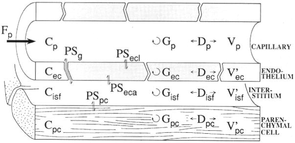
Schematic representation of four-region axially distributed single capillary-tissue unit composed of plasma at flow F_p and surrounding capillary endothelial wall, interstitial fluid space, and parenchymal cells of the organ. The Vs are volumes of distribution. Barrier conductances are given by the permeability surface area product (PS). The capillary wall is permeated by passive transport through interendothelial clefts as well as transport across the endothelial plasmalemma. Axial dispersion (D) approximately accounts for intravascular velocity profiles and molecular diffusion. Intra-regional reactions or metabolic consumption are given by the “gulosities” or clearances (G). p, plasma; g, interendothelial cleft or gap PS; ecl, luminal surface of endothelial cell; ec, endothelial cell; isf, interstitium; eca, antiluminal surface of endothelial cell; pc, parenchymal cell.

In the plasma, assuming plug or piston flow,

$$\frac{\partial {\mathrm{C}}_{\mathrm{p}}}{\partial \mathrm{t}}=-\frac{{\mathrm{F}}_{\mathrm{p}}\mathrm{L}}{{\mathrm{V}}_{\mathrm{p}}}\cdot \frac{\partial {\mathrm{C}}_{\mathrm{p}}}{\partial \mathrm{x}}-\frac{{\text{PS}}_{\mathrm{g}}}{{\mathrm{V}}_{\mathrm{p}}}({\mathrm{C}}_{\mathrm{p}}-{\mathrm{C}}_{\text{isf}})-\frac{{\text{PS}}_{\text{ec}l}}{{\mathrm{V}}_{\mathrm{p}}}({\mathrm{C}}_{\mathrm{p}}-{\mathrm{C}}_{\text{ec}})-\frac{{\mathrm{G}}_{\mathrm{p}}}{{\mathrm{V}}_{\mathrm{p}}}{\mathrm{C}}_{\mathrm{p}}+{\mathrm{D}}_{\mathrm{p}}\frac{{\partial }^2{\mathrm{C}}_{\mathrm{p}}}{\partial {\mathrm{x}}^2}\cdot$$ (1)

In endothelial cells,

$$\frac{\partial {\mathrm{C}}_{\text{ec}}}{\partial \mathrm{t}}=-\frac{{\text{PS}}_{\text{ec}l}}{{\mathrm{V}}_{\text{ec}}^{\prime }}({\mathrm{C}}_{\text{ec}}-{\mathrm{C}}_{\mathrm{p}})-\frac{{\text{PS}}_{\text{eca}}}{{\mathrm{V}}_{\text{ec}}^{\prime }}({\mathrm{C}}_{\text{ec}}-{\mathrm{C}}_{\text{isf}})-\frac{{\mathrm{G}}_{\text{ec}}}{{\mathrm{V}}_{\text{ec}}^{\prime }}\cdot {\mathrm{C}}_{\text{ec}}+{\mathrm{D}}_{\text{ec}}\frac{{\partial }^2{\mathrm{C}}_{\text{ec}}}{\partial {\mathrm{x}}^2}\cdot$$ (2)

In interstitial fluid,

$$\frac{\partial {\mathrm{C}}_{\text{isf}}}{\partial \mathrm{t}}=-\frac{{\text{PS}}_{\mathrm{g}}}{{\mathrm{V}}_{\text{isf}}^{\prime }}({\mathrm{C}}_{\text{isf}}-{\mathrm{C}}_{\mathrm{p}})-\frac{{\text{PS}}_{\text{eca}}}{{\mathrm{V}}_{\text{isf}}^{\prime }}({\mathrm{C}}_{\text{isf}}-{\mathrm{C}}_{\text{ec}})-\frac{{\text{PS}}_{\text{pc}}}{{\mathrm{V}}_{\text{isf}}^{\prime }}({\mathrm{C}}_{\text{isf}}-{\mathrm{C}}_{\text{pc}})-\frac{{\mathrm{G}}_{\text{isf}}}{{\mathrm{V}}_{\text{isf}}^{\prime }}{\mathrm{C}}_{\text{isf}}+{\mathrm{D}}_{\text{isf}}\frac{{\partial }^2{\mathrm{C}}_{\text{isf}}}{\partial {\mathrm{x}}^2}\cdot$$ (3)

In parenchymal cells,

$$\frac{\partial {\mathrm{C}}_{\text{pc}}}{\partial \mathrm{t}}=-\frac{{\text{PS}}_{\text{pc}}}{{\mathrm{V}}_{\text{pc}}^{\prime }}({\mathrm{C}}_{\text{pc}}-{\mathrm{C}}_{\text{isf}})-\frac{{\mathrm{G}}_{\text{pc}}}{{\mathrm{V}}_{\text{pc}}^{\prime }}{\mathrm{C}}_{\text{pc}}+{\mathrm{D}}_{\text{pc}}\frac{{\partial }^2{\mathrm{C}}_{\text{pc}}}{\partial {\mathrm{x}}^2}\cdot$$ (4)

Scaling by the ratios of distribution volumes (γ_rs) and summing give the conservation expression:

$$-\sum {\mathrm{D}}_{\mathrm{r}}{\gamma }_{\mathrm{r}}\frac{{\partial }^2{\mathrm{C}}_{\mathrm{r}}}{\partial {\mathrm{x}}^2}+\sum {\gamma }_{\mathrm{r}}\frac{\partial {\mathrm{C}}_{\mathrm{r}}}{\partial \mathrm{t}}+\alpha \frac{\partial {\mathrm{C}}_{\mathrm{p}}}{\partial \mathrm{x}}+\sum \frac{{\mathrm{G}}_{\mathrm{r}}{\mathrm{C}}_{\mathrm{r}}}{{\mathrm{V}}_{\mathrm{p}}}=0.$$ (5)

The terms are as follows: C, concentration in moles per cubic centimeter; C_r(x, t), concentration in region r at position × along the unit, at time t (within regions, the radial gradients are considered negligible, an assumption that is justified in well-perfused organs); D, axial diffusion or dispersion coefficient in centimeters squared per second; F_p, flow in (milliliters per gram) per second, defined as flow per gram of tissue (including the capillary); h(t), transport function or normalized outflow dilution curve: h(t) = F_p×C(t)/q₀, where q₀ is the amount of tracer in the injectate in moles; the terms h_R, h_E, and h_D designate the intravascular reference tracer (R), the extracellular reference tracer (E), the test diffusible solute (D) that enter cells, respectively; E(t), extraction relative to the reference intravascular tracer: E(t) = 1 − h_D(t)/h_R(t) for the test solute and E_E(t) = 1 − h_E(t)/h_R(t) for the extracellular (second) reference solute; G, regional clearance in (milliliters per gram) per second (gulosity or first-order consumption, removal by binding, sequestration, or transformation); ISF, interstitial fluid space; L, capillary length (arbitrary) in centimeters (in the heart, 0.05 – 0.1 cm); N, number of axial segments used for numerical solutions; PS, permeability-surface area product in (milliliters per gram) per second (assumed constant axially in the equations); RD, relative dispersion (RD = SD/mean of a distribution); t, time in seconds; U(t), extraction of the test solute relative to the extracellular reference solute: U(t) = 1 − h_D(t)/h_E(t); V, volume of a region in milliliters per gram; V′, volume of distribution in a region in milliliters per gram equal to region-to-plasma partition coefficient (dimensionless) times the anatomic volume V, in milliliters per gram (a ratio ${\mathrm{V}}_{\mathrm{r}}^{\prime }/{\mathrm{V}}_{\mathrm{r}}$ different from 1.0 would indicate an asymmetric nonpassive membrane transport process; ${\mathrm{V}}_{\text{pc}}^{\prime }/{\mathrm{V}}_{\text{pc}}>1$ indicates parenchymal cell accumulation; and ${\mathrm{V}}_{\text{pc}}^{\prime }/{\mathrm{V}}_{\text{pc}}<1$ indicates that extrusion is faster than entry); α is plasma velocity in centimeters per second; γ_r, ratio of volume of distribution in region to that in plasma, ${\mathrm{V}}_{\mathrm{r}}^{\prime }/{\mathrm{V}}_{\mathrm{p}}$; and x, distance along capillary in centimeters. The concentrations and the parameters D, PS, and G, and for gulosity (consumption), are subscripted as defined in the legend to Figure 1. For general statements, we use the subscripts r, region, where r refers to p, ec, isf, or pc.

Partial differential equations require defining both initial conditions and boundary conditions. The initial conditions for all of the solutions shown were the concentrations were zero in all regions. The boundary condition at the entrance to the capillary is essential for defining the rate of entry into the capillary for each of the solutes, and is: $-\frac{{\mathrm{F}}_{\mathrm{p}}\mathrm{L}}{{\mathrm{V}}_{\mathrm{p}}}\cdot \frac{\partial \mathrm{C}}{\partial \mathrm{x}}+{\mathrm{D}}_{\mathrm{p}}\frac{{\partial }^2\mathrm{C}}{\partial {\mathrm{x}}^2}=0$. The other boundary conditions are called reflecting boundary conditions and prevent diffusion out of the regions; at all the upstream and downstream boundaries, at x = 0 and x = L, the derivatives are set to zero: $\mathrm{d}\mathrm{C}/\mathrm{d}\mathrm{x}=0$.

These four-region equations extend the two-region axially dispersive model of Bassingthwaighte⁴ and the three-region axially dispersive model of Kuikka et al.⁵ Note that the existence of direct plasma-to-isf exchanges, bypassing the endothelial cell, makes this model differ from one with a series of concentric volumes. The axial dispersion (molecular diffusion plus eddies and other sources of axial mixing in the vascular space) is substantial in large vessels and capillaries, although it is similar for molecules of widely differing size.¹⁸ RDs in arteries are about 16–20%, and similar dispersions are observed even if not measured accurately in capillaries.¹⁹ We provide a numerical solution for the complete single-capillary model and a closed form “pseudoanalytic” expression for the model that omits only axial diffusion.

The multicapillary model

For practical application, such a model needs to be incorporated into a multicapillary configuration. The organ is considered to be made up of a set of parallel independent capillary tissue units, as described by Levin et al,²⁰ but other configurations could be used as readily. In such a configuration, the overall set of capillary tissue units would have an impulse response [h_C(t)] composed of the weighted sum of individual capillary impulse responses [h_Ci(t)s] thus,

$${\mathrm{h}}_{\mathrm{c}}\left(\mathrm{t}\right)=\sum _{\mathrm{i}}{\mathrm{w}}_{\mathrm{i}}{\mathrm{f}}_{\mathrm{i}}\Delta {\mathrm{f}}_{\mathrm{i}}{\mathrm{h}}_{{\mathrm{C}}_{\mathrm{i}}}(\mathrm{t})$$

where the relative flow f_i, (dimensionless) is the regional flow divided by the mean flow to the whole organ, w_i is the weighting or probability density function of the relative f_is, and Δf_i is the class width for the distribution function of relative flows. The area of the density function, Σw_iΔf_i, is 1.0, and the mean regional flow, Σw_if_iΔf_i, also equals 1. The product w_if_iΔf_i gives the fraction of the total flow passing through each capillary tissue unit with relative flow f_i. The actual flow in the i^th capillary is f_i F, where F is the average flow in (milliliters per gram) per second for the whole organ. In such a model formulation, the dispersion in the large vessels of the vascular system is given by the transport function (h_LV) so that the total intravascular transport from injection point in the inflow to sampling point in the outflow is the convolution (*) of the large vessel and the aggregate capillary-tissue transport functions so that h(t) for the whole organ equals h_LV*h_C. (When using the capillary-tissue model as a differential operator, with h_LV as the input function, the convolution is accomplished without any formal convolution and without even a single multiplication or extra computation.)

Methods of Solutions for the Model Equations

Three methods of obtaining solutions to the single capillary-tissue unit model are considered. The first is an analytic solution via Laplace transforms. This must be translated into numerical form to be used in practice, and we shall see that this particular analytic solution is cumbersome to translate. Two numerical methods of solution, both based on a sliding fluid element or Lagrangian approach, are presented as more practical approaches based on earlier two- and three-region models.^4,6

Continuous analytical solution

This is a closed-form analytic solution based on reduction of Equations 1–4 to omit axial diffusion or dispersion. The velocity profile in the intracapillary region is thereby assumed to be uniform, piston flow, or plug flow, which is dispersionless. The approach to the solution is similar to those used by Sangren and Sheppard²¹ for a two-region model and by Rose et al¹ for a three-region model.

The analytic solution for the four-region model proposed here, without axial diffusion (all Ds = 0), may be obtained by Laplace transform. For compactness in notation, we set the regional concentrations as follows: C_p ≡ u, C_ec ≡ v, C_isf ≡ w, and C_pc ≡ z. The plasma velocity, α, is given by

$$\frac{{\mathrm{F}}_{\mathrm{p}}\mathrm{L}}{{\mathrm{V}}_{\mathrm{p}}}\equiv \alpha$$ (6)

The volume ratios are

$$\frac{{\mathrm{V}}_{\text{ec}}^{\prime }}{{\mathrm{V}}_{\mathrm{p}}}\equiv {\gamma }_{\text{ec}},\frac{{\mathrm{V}}_{\text{isf}}^{\prime }}{{\mathrm{V}}_{\mathrm{p}}}\equiv {\gamma }_{\text{isf}},\text{and}\frac{{\mathrm{V}}_{\text{pc}}^{\prime }}{{\mathrm{V}}_{\mathrm{p}}}\equiv {\gamma }_{\text{pc}}$$ (7)

The rate coefficients are

$$\frac{{\text{PS}}_{\mathrm{g}}}{{\mathrm{V}}_{\mathrm{p}}}\equiv k_1,\frac{{\text{PS}}_{\text{ec}l}}{{\mathrm{V}}_{\mathrm{p}}}\equiv k_2,\frac{{\text{PS}}_{\text{eca}}}{{\mathrm{V}}_{\mathrm{p}}}\equiv k_4,\text{and}\frac{{\text{PS}}_{\text{pc}}}{{\mathrm{V}}_{\mathrm{p}}}\equiv k_6$$ (8)

$$\frac{{\mathrm{G}}_{\mathrm{p}}}{{\mathrm{V}}_{\mathrm{p}}}\equiv k_3,\frac{{\mathrm{G}}_{\text{ec}}}{{\mathrm{V}}_{\mathrm{p}}}\equiv k_5,\frac{{\mathrm{G}}_{\text{isf}}}{{\mathrm{V}}_{\mathrm{p}}}\equiv k_7,\text{and}\frac{{\mathrm{G}}_{\text{pc}}}{{\mathrm{V}}_{\mathrm{p}}}\equiv k_8$$ (9)

Equations 1–4 become

$$\frac{\partial \mathrm{u}}{\partial \mathrm{t}}+\alpha \frac{\partial \mathrm{u}}{\partial \mathrm{x}}=-k_1(\mathrm{u}-\mathrm{w})-k_2(\mathrm{u}-\mathrm{v})-k_3\mathrm{u}$$ (10)

$${\gamma }_{\text{ec}}\frac{\partial \mathrm{v}}{\partial \mathrm{t}}=-k_2(\mathrm{v}-\mathrm{u})-k_4(\mathrm{v}-\mathrm{w})-k_5\mathrm{v}$$ (11)

$${\gamma }_{\text{isf}}\frac{\partial \mathrm{w}}{\partial \mathrm{t}}=-k_1(\mathrm{w}-\mathrm{u})-k_4(\mathrm{w}-\mathrm{v})-k_6(\mathrm{w}-\mathrm{z})-k_7\mathrm{w}$$ (12)

$${\gamma }_{\text{pc}}\frac{\partial \mathrm{z}}{\partial \mathrm{t}}=-k_6(\mathrm{z}-\mathrm{w})-k_8\mathrm{z}.$$ (13)

To obtain the impulse response or transport function for this system, the input at t = 0 is a unit spike or a spatial Dirac delta function δ(x) at the arterial end of the capillary. Thus, the initial conditions are

$$\mathrm{u}(\mathrm{x},0)=\delta (\mathrm{x})$$ (14)

$$\mathrm{v}(\mathrm{x},0)=\mathrm{w}(\mathrm{x},0)=\mathrm{z}(\mathrm{x},0)=0$$ (15)

Let the Laplace transforms of u, v, w, and z be U, V, W, Z; for example,

$$\mathrm{U}(\mathrm{x},\mathrm{s})\equiv L\mathrm{u}(\mathrm{x},\mathrm{t})\equiv {\int }_0^{\infty }\mathrm{u}(\mathrm{x},\mathrm{t}){\mathrm{e}}^{-\text{st}}\text{dt}$$ (16)

Then Equations 10–13 yield

$$\text{sU}+\alpha \frac{\text{dU}}{\text{dx}}=-k_1(\mathrm{U}-\mathrm{W})-k_2(\mathrm{U}-\mathrm{V})-k_3\mathrm{U}+\delta (\mathrm{x})$$ (17)

$${\gamma }_{\text{ec}}\text{sV}=-k_2(\mathrm{V}-\mathrm{U})-k_4(\mathrm{V}-\mathrm{W})-k_5\mathrm{V}$$ (18)

$${\gamma }_{\text{isf}}\text{sW}=-k_1(\mathrm{W}-\mathrm{U})-k_4(\mathrm{W}-\mathrm{V})-k_6(\mathrm{W}-\mathrm{Z})-k_7\mathrm{W}$$ (19)

$${\gamma }_{\text{pc}}\text{sZ}=-k_6(\mathrm{Z}-\mathrm{W})-k_8\mathrm{Z}$$ (20)

From Equations 18–20, we express V, W, and Z in terms of U. After some algebraic manipulation, we find

$$\mathrm{V}=\frac{k_2\mathrm{D}+(k_1{\mathrm{B}}_1+k_2{k}_4){\mathrm{B}}_2{k}_4}{{\mathrm{B}}_1\mathrm{D}}\mathrm{U}$$ (21)

$$\mathrm{W}=\frac{(k_1{\mathrm{B}}_1+k_2{k}_4){\mathrm{B}}_2}{\mathrm{D}}\mathrm{U}$$ (22)

$$\mathrm{Z}=\frac{(k_1{\mathrm{B}}_1+k_2{k}_4)k_6}{\mathrm{D}}\mathrm{U}$$ (23)

where B₁ ≡ γ_ecs + k₂ + k₄ + k₅, B₂ ≡ γ_pcs + k₆ + k₈, B₃, ≡ γ_isfs + k₁ + k₄ + k₆ + k₇, and $\mathrm{D}\equiv {\mathrm{B}}_1({\mathrm{B}}_2{\mathrm{B}}_3-k_6^2)-k_4^2{\mathrm{B}}_2$ On substitution into Equation 17, an ordinary differential equation in U is found:

$$\alpha \frac{\text{dU}}{\text{dx}}+\mathrm{M}(\mathrm{s})\mathrm{U}=\delta (\mathrm{x})$$ (24)

where

$$\mathrm{M}(\mathrm{s})\equiv \mathrm{s}+k_1+k_2+k_3-\frac{k_1^2{\mathrm{B}}_1{\mathrm{B}}_2+2k_1{k}_2{k}_4{\mathrm{B}}_2+k_2^2{\mathrm{B}}_2{\mathrm{B}}_3-k_2^2{k}_6^2}{\mathrm{D}}$$ (25)

The last term of Equation 25 can be written into partial fractions such that

$$\mathrm{M}(\mathrm{s})=\mathrm{s}+{\beta }_0-\frac{{\beta }_1}{\mathrm{s}-{\mathrm{s}}_1}-\frac{{\beta }_2}{\mathrm{s}-{\mathrm{s}}_2}-\frac{{\beta }_3}{\mathrm{s}-{\mathrm{s}}_3}$$ (26)

where β₀ ≡ k₁ + k₂ + k₃, and the s₁, s₂, and s₃ are the three (distinct) roots of D, and

$${\beta }_{\mathrm{i}}=\underset{\mathrm{s}\to {\mathrm{S}}_{\mathrm{i}}}{\text{lim}}(\mathrm{s}-{\mathrm{s}}_{\mathrm{i}})\frac{k_1^2{\mathrm{B}}_1{\mathrm{B}}_2+2k_1{k}_2{k}_4{\mathrm{B}}_2+k_2^2{\mathrm{B}}_2{\mathrm{B}}_3-k_2^2{k}_6^2}{\mathrm{D}}$$ (27)

where i = 1,2,3.

The solution to Equation 24 is

$$\mathrm{U}\left(\mathrm{x},\mathrm{s}\right)=\frac{1}{\alpha }\mathrm{S}(\mathrm{x})\cdot {\mathrm{e}}^{\frac{-\text{sx}}{\alpha }}\cdot {\mathrm{e}}^{\frac{-{\beta }_0\mathrm{x}}{\alpha }}\cdot {\mathrm{e}}^{\frac{{\beta }_1\mathrm{x}}{\alpha \left(\mathrm{s}-{\mathrm{s}}_1\right)}}\cdot {\mathrm{e}}^{\frac{{\beta }_2\mathrm{x}}{\alpha \left(\mathrm{s}-{\mathrm{s}}_2\right)}}\cdot {\mathrm{e}}^{\frac{{\beta }_3\mathrm{x}}{\alpha \left(\mathrm{s}-{\mathrm{s}}_3\right)}}$$ (28)

where S(x) is the unit step function. In order to invert Equation 28, we note^22,23

$$L^{-1}({\mathrm{e}}^{\frac{\mu }{8}}-1)=\sqrt{\frac{\mu }{\mathrm{t}}}{\mathrm{I}}_1\left(2\sqrt{\mu \mathrm{t}}\right)$$ (29)

where I₁ is the first-order modified Bessel function. If we define a function F_i,

$${\mathrm{F}}_{\mathrm{i}}\equiv {\mathrm{e}}^{\frac{{\beta }_1\mathrm{x}}{\alpha \left(\mathrm{s}-{\mathrm{s}}_1\right)}}-1$$ (30)

then

$$L^{-1}{\mathrm{F}}_{\mathrm{i}}={\mathrm{e}}^{{\mathrm{s}}_{\mathrm{i}}\mathrm{t}}{L}^{-1}({\mathrm{e}}^{\frac{{\beta }_1\mathrm{x}}{\alpha \mathrm{s}}}-1)={\mathrm{e}}^{{\mathrm{s}}_{\mathrm{i}}\mathrm{t}}\sqrt{\frac{{\mu }_{\mathrm{i}}}{\mathrm{t}}}{\mathrm{I}}_1\left(2\sqrt{{\mu }_{\mathrm{i}}\mathrm{t}}\right)$$ (31)

$${\mu }_{\mathrm{i}}\equiv {\beta }_1\mathrm{x}/\alpha$$ (32)

Thus, by use of T ≡ t−x/α and S(x) or S(T) to denote the unit step function

$$\begin{array}{l}\mathrm{u}(\mathrm{x},\mathrm{t})=L^{-1}\mathrm{U}(\mathrm{x},\mathrm{s})\\ =\frac{\mathrm{S}(\mathrm{x})}{\alpha }{\mathrm{e}}^{\frac{-{\beta }_0\mathrm{x}}{\alpha }}{L}^{-1}{\mathrm{e}}^{\frac{-\text{sx}}{\alpha }}\left[\left(1+{\mathrm{F}}_1\right)\left(1+{\mathrm{F}}_2\right)\left(1+{\mathrm{F}}_3\right)\right]\\ =\frac{\mathrm{S}(\mathrm{x})}{\alpha }{\mathrm{e}}^{\frac{-{\beta }_0\mathrm{x}}{\alpha }}{L}^{-1}{\mathrm{e}}^{\frac{-\text{sx}}{\alpha }}\left[1+\left({\mathrm{F}}_1+{\mathrm{F}}_2+{\mathrm{F}}_3+{\mathrm{F}}_1{\mathrm{F}}_2{+\mathrm{F}}_1{\mathrm{F}}_3+{\mathrm{F}}_2{\mathrm{F}}_3+{\mathrm{F}}_1{\mathrm{F}}_2{\mathrm{F}}_3\right)\right]\\ =\frac{\mathrm{S}(\mathrm{x})}{\alpha }{\mathrm{e}}^{\frac{-{\beta }_0\mathrm{x}}{\alpha }}\left[\delta (\mathrm{T})+\mathrm{S}(\mathrm{T})\left(L^{-1}{\mathrm{F}}_1+L^{-1}{\mathrm{F}}_2+L^{-1}{\mathrm{F}}_3+L^{-1}{\mathrm{F}}_1\ast L^{-1}{\mathrm{F}}_2+L^{-1}{\mathrm{F}}_1\ast L^{-1}{\mathrm{F}}_3+L^{-1}{\mathrm{F}}_2\ast L^{-1}{\mathrm{F}}_3+L^{-1}{\mathrm{F}}_1\ast L^{-1}{\mathrm{F}}_2\ast L^{-1}{\mathrm{F}}_3\right)\right]\end{array}$$ (33)

where t→T. The asterisks, *, denote convolution.

Finally, the time domain solution for the intravascular concentration at any point x is:

$$\mathrm{u}(\mathrm{x},\mathrm{t})=\frac{\mathrm{S}(\mathrm{x})}{\alpha }{\mathrm{e}}^{\frac{-{\beta }^0\mathrm{x}}{\alpha }}\{\delta (\mathrm{T})+\mathrm{S}(\mathrm{T})[\sum _{\mathrm{i}=1}^3{\mathrm{e}}^{{\mathrm{s}}_{\mathrm{i}}\mathrm{T}}\sqrt{\frac{{\mu }_{\mathrm{i}}}{\mathrm{T}}}{\mathrm{I}}_1(2\sqrt{{\mu }_{\mathrm{i}}\mathrm{T}})+{\int }_0^{\mathrm{T}}{\mathrm{e}}^{{\mathrm{s}}_1\left(\mathrm{T}-\mathrm{r}\right)}\sqrt{\frac{{\mu }_1}{\mathrm{T}-\mathrm{r}}}{\mathrm{I}}_1[2\sqrt{{\mu }_1(\mathrm{T}-\mathrm{r})}]{\mathrm{e}}^{{\mathrm{s}}_2\mathrm{r}}\sqrt{\frac{{\mu }_2}{\mathrm{r}}}{\mathrm{I}}_1(2\sqrt{{\mu }_2\mathrm{r}})\text{dr}+{\int }_0^{\mathrm{T}}{\mathrm{e}}^{{\mathrm{s}}_2(\mathrm{T}-\mathrm{r})}\sqrt{\frac{{\mu }_2}{\mathrm{T}-\mathrm{r}}}{\mathrm{I}}_1[2\sqrt{{\mu }_2(\mathrm{T}-\mathrm{r})}]{\mathrm{e}}^{{\mathrm{s}}_3\mathrm{r}}\sqrt{\frac{{\mu }_3}{\mathrm{r}}}{\mathrm{I}}_1\left(2\sqrt{{\mu }_3\mathrm{r}}\right)\text{dr}+{\int }_0^{\mathrm{T}}{\mathrm{e}}^{{\mathrm{s}}_3(\mathrm{T}-\mathrm{r})}\sqrt{\frac{{\mu }_3}{\mathrm{T}-\mathrm{r}}}{\mathrm{I}}_1[2\sqrt{{\mu }_3(\mathrm{T}-\mathrm{r})}]{\mathrm{e}}^{{\mathrm{s}}_2\mathrm{r}}\sqrt{\frac{{\mu }_1}{\mathrm{r}}}{\mathrm{I}}_1\left(2\sqrt{{\mu }_1\mathrm{r}}\right)\text{dr}+{\int }_0^{\mathrm{T}}{\mathrm{e}}^{{\mathrm{s}}_1(\mathrm{T}-\mathrm{p})}\sqrt{\frac{{\mu }_1}{\mathrm{T}-\mathrm{p}}}{\mathrm{I}}_1[2\sqrt{{\mu }_1(\mathrm{T}-\mathrm{p})}]{\int }_o^{\mathrm{p}}{\mathrm{e}}^{{\mathrm{s}}_2(\mathrm{p}-\mathrm{r})}\sqrt{\frac{{\mu }_2}{\mathrm{p}-\mathrm{r}}}{\mathrm{I}}_1[2\sqrt{{\mu }_2(\mathrm{p}-\mathrm{r})}]\times {\mathrm{e}}^{{\mathrm{s}}_3\mathrm{r}}\sqrt{\frac{{\mu }_3}{\mathrm{r}}}{\mathrm{I}}_1(2\sqrt{{\mu }_3\mathrm{r}})\text{dr}\text{dp}]\}$$ (34)

The solution, Equation 34, is exact. Similar expressions can be derived for the other regions. It may be tedious to evaluate the double integral, the last term. At the outflow, x = L, the solution is composed of a leading spike occurring at one capillary transit time, t̄_p = V_p/F_p, the first term of Equation 34, followed by a tail function described by the terms windowed by S(T). The spike is the transmitted or nonextracted part of the injected tracer, which has been scaled down by the losses of tracer by permeation through clefts and across the luminal surface of the endothelial cell and by intracapillary reaction:

$${\mathrm{e}}^{\frac{-{\beta }_0\mathrm{L}}{\alpha }}={\mathrm{e}}^{(-k_1+k_2+k_3){\mathrm{V}}_{\mathrm{p}}/{\mathrm{F}}_{\mathrm{p}}}={\mathrm{e}}^{-({\text{PS}}_{\mathrm{g}}+{\text{PS}}_{\text{ec}l}+{\mathrm{G}}_{\mathrm{p}})/{\mathrm{F}}_{\mathrm{p}}}$$

When PS_ecl and G_p are zero (no endothelial luminal surface permeation and no consumption in the plasma region), this is identical to the spike term given by Sangren and Sheppard²¹ and Rose et al.¹ Crone's¹⁰ measure of instantaneous extraction, E(t) = 1 − h_D(t)/h_R(t), serves as a useful measure of early-time events; the single capillary approximation is (PS_g + PS_ecl + G_p) = − F_plog_e(1 − E) until reflux occurs from extravascular regions into the plasma.

The curve at the exit from the capillary, u(L,t), gives the equivalent to an observed outflow dilution curve. For an intravascular nonmetabolized reference tracer, the outflow response to an impulse input is u(L,t) = δ(t−T). For the permeant tracer h_D(t) upon convolution, the asterisk, with a transport function h_LV(t) representing arterial and venous transport:

$${\mathrm{h}}_{\mathrm{D}}(\mathrm{t})={\mathrm{h}}_{\text{LV}}(\mathrm{t})\ast \mathrm{u}(\mathrm{L},\mathrm{t})$$

We avoid convolution in numerical solutions by providing h_LV(t) as the input to a differential operator describing the system and by obtaining h_D(t) with the same number of operations as required for u(L,t) alone.

In the degenerate case of a three-region model without entry into endothelial cells, we set PS_ecl = PS_eca = G_ec = 0 or k₂ = k₄ = k₅ = 0. Then we find V = Lv = 0 and Equation 25 is supplanted by

$$\begin{array}{l}\mathrm{M}(\mathrm{s})=\mathrm{s}+k_1+k_3-\frac{k_1^2{\mathrm{B}}_2}{{\mathrm{B}}_2{\mathrm{B}}_3-k_6^2}\\ =\mathrm{s}+{\beta }_0-\frac{{\beta }_1}{\mathrm{s}-{\mathrm{s}}_1}-\frac{{\beta }_2}{\mathrm{s}-{\mathrm{s}}_2}\end{array}$$ (35)

where s₁ and s₂ are the two roots of ${\mathrm{B}}_2{\mathrm{B}}_3-{\mathit{\text{k}}}_6^2=0$, and terms using β₃ and s₃ in Equations 26–28 are gone. Equation 34 then reduces almost to the three-region model derived by Rose et al¹ but differs from it because of retention of terms for reaction, the Gs in plasma and isf as well as in parenchymal cells.⁶ In the present work, we have used the relation of Equation 29 to avoid the infinite series used by Rose et al¹ in their approach to the solution. However, evaluating the quadratic ${\mathrm{B}}_2{\mathrm{B}}_3-{\mathit{\text{k}}}_6^2=0$, and the Bessel functions is unavoidable.

Steady-state solutions for a constant concentration at the inflow are given in the Appendix. They account for standing gradients in concentrations in all the regions when there is consumption in any of them.

Sliding fluid element algorithm, an efficient numerical method

In this approach, the strategy for describing intravascular velocity is the same whether axial diffusion is considered or not. With D_x = 0, it is conceptually analogous to the analytical solution (Equation 34). The approach, suggested originally by J.L. Stephenson²⁴ and used in an earlier model,⁴ has the advantage of accounting for intravascular and extravascular dispersion or diffusion to give a good but approximate representation of the dispersion in the plasma phase relative to that in the extravascular regions. An abbreviated outline will be presented here. The details and documentation of the accuracy are provided for a three-region model by Bassingthwaighte et al.⁶

The capillary (and adjacent tissue regions) is divided into N equal lengths, Δx = L/N, such that the solution time step is $\Delta \mathrm{t}={\mathrm{V}}_{\mathrm{p}}^{\prime }/({\mathrm{F}}_{\mathrm{p}}\times \mathrm{N})$, and the capillary plasma transit time (t̄_p) is NΔt. At the start of each time interval, the fluid contents of each capillary segment are advanced by one segment such that the concentration in the (i +1)^th element is replaced by the concentration in the i^th element and the outflow concentration is replaced by that in the last segment:

$${\mathrm{C}}_{\mathrm{p}}({\mathrm{x}}_{\mathrm{i}+1},\mathrm{j}\Delta {\mathrm{t}}_{+})={\mathrm{C}}_{\mathrm{p}}({\mathrm{x}}_{\mathrm{i}},\mathrm{j}\Delta {\mathrm{t}}_{-})$$ (36)

$${\mathrm{C}}_{\mathrm{p}}(\mathrm{L},\mathrm{t})={\mathrm{C}}_{\text{out}}(\mathrm{j}\Delta {\mathrm{t}}_{+})={\mathrm{C}}_{\mathrm{p}}({\mathrm{x}}_{\mathrm{N}},\mathrm{j}\Delta {\mathrm{t}}_{-})$$ (37)

where jΔt₊ is time at the beginning of the j^th time step and jΔt₋ is time at the end of the previous interval. This is the instant of the sliding phase. Thereafter, during the interval jΔt₊ to (j + 1)Δt₋ exchanges occur in accord with first-order processes between the radially arranged volume elements of the model, which describe exchange across barriers. This is the permeation phase of the step. Linear, first-order exchanges are appropriate for tracers in the presence of constant concentrations of another substance but not with saturable transporters when the nontracer concentrations are changing.¹⁵

Two methods of providing numerical solutions to the sliding element model are to be described and compared with other methods. The first of these gives a local analytical solution for the four radial regions during each time step for each axial segment and is applicable to the situation in which the axial diffusion coefficients are all zero, as is the case for the analytical solution given in Equation 34.

Sliding fluid element model with local analytical solution steps

We solve analytically the concentrations in the four regions at each axial position during the permeation phase of radially linked compartments to obtain the values u, v, w, and z at the end of each time interval, which are the initial conditions for the next time step. The differential equations are similar to Equations 10–13 but omit the convection term accounted for by the slide:

$$\frac{\text{du}}{\text{dt}}=-k_1(\mathrm{u}-\mathrm{w})-k_2(\mathrm{u}-\mathrm{v})-k_3\mathrm{u}$$ (38)

$${\gamma }_{\text{ec}}\frac{\text{dv}}{\text{dt}}=-k_2(\mathrm{v}-\mathrm{u})-k_4(\mathrm{v}-\mathrm{w})-k_5\mathrm{v}$$ (39)

$${\gamma }_{\text{isf}}\frac{\text{dw}}{\text{dt}}=-k_1(\mathrm{w}-\mathrm{u})-k_4(\mathrm{w}-\mathrm{v})-k_6(\mathrm{w}-\mathrm{z})-k_7\mathrm{w}$$ (40)

$${\gamma }_{\text{pc}}\frac{\text{dz}}{\text{dt}}=-k_6(\mathrm{z}-\mathrm{w})-k_8\mathrm{z}$$ (41)

Owing to the linearity of Equations 38–41, we have the general solution

$$\underset{\sim }{\mathrm{U}}(\mathrm{t}+\Delta \mathrm{t})={\mathrm{e}}^{\underset{\sim }{\mathrm{A}}\Delta \mathrm{t}}\underset{\sim }{\mathrm{U}}(\mathrm{t})$$ (42)

where Ṵ is the concentration vector (u, v, w, z)^T and A̰ is the 4×4 matrix

$$\underset{\sim }{\mathrm{A}}=\left[\begin{array}{cccc}-k_1-k_2-k_3& k_2& k_1& 0\\ \frac{k_2}{{\gamma }_{\text{ec}}}& -\frac{k_2+k_4+k_5}{{\gamma }_{\text{ec}}}& \frac{k_4}{{\gamma }_{\text{ec}}}& 0\\ \frac{k_1}{{\gamma }_{\text{isf}}}& \frac{k_4}{{\gamma }_{\text{isf}}}& -\frac{k_1+k_4+k_6+k_7}{{\gamma }_{\text{isf}}}& \frac{k_6}{{\gamma }_{\text{isf}}}\\ 0& 0& \frac{k_6}{{\gamma }_{\text{pc}}}& -\frac{k_6+k_8}{{\gamma }_{\text{pc}}}\end{array}\right]$$ (43)

The e^A̰Δt can be computed by the eigenvalue and eigenvector approach, the analytical approach:

$${\mathrm{e}}^{\underset{\sim }{\mathrm{A}}\Delta \mathrm{t}}=\underset{\sim }{\Phi }\mathrm{e}\underset{\sim }{\Lambda }\Delta \mathrm{t}{\underset{\sim }{\Phi }}^{-1}=({\underset{\sim }{\phi }}_1,{\underset{\sim }{\phi }}_2,{\underset{\sim }{\phi }}_3,{\underset{\sim }{\phi }}_4){\mathrm{e}}^{\underset{\sim }{\Lambda }\Delta \mathrm{t}}{({\underset{\sim }{\phi }}_1,{\underset{\sim }{\phi }}_2,{\underset{\sim }{\phi }}_3,{\underset{\sim }{\phi }}_4)}^{-1}$$ (44)

where Λ̰ is a 4×4 diagonal matrix with eigenvalue λ₁,λ₂,λ₃, and λ₄ on the diagonal, corresponding to the eigenvectors ϕ̰₁, ϕ̰₂, ϕ̰₃, and ϕ̰₄, respectively.

The eigenvalues λ_i for i = 1, 2, 3, 4 can be found by solving for the roots of the following polynomial:

$$\left|\underset{\sim }{\mathrm{A}}-\underset{\sim }{\lambda }\mathrm{I}\right|=0$$ (45)

The eigenvectors ϕ_i satisfy

$$(\underset{\sim }{\mathrm{A}}-{\lambda }_{\mathrm{j}}\mathrm{I}){\underset{\sim }{\phi }}_{\mathrm{i}}=\underset{\sim }{0}$$ (46)

where 0̰ = (0, 0, 0, 0)^T.

With the consideration of the sliding, we can write Equation 42 as

$$\begin{array}{lll}\left[\begin{array}{l}\mathrm{u}({\mathrm{x}}_{\mathrm{i}},\mathrm{t}+\Delta \mathrm{t})\\ \mathrm{v}({\mathrm{x}}_{\mathrm{i}},\mathrm{t}+\Delta \mathrm{t})\\ \mathrm{w}({\mathrm{x}}_{\mathrm{i}},\mathrm{t}+\Delta \mathrm{t})\\ \mathrm{z}({\mathrm{x}}_{\mathrm{i}},\mathrm{t}+\Delta \mathrm{t})\end{array}\right]& =\underset{\sim }{\Phi }{\mathrm{e}}^{\underset{\sim }{\Lambda }\Delta \mathrm{t}}{\underset{\sim }{\Phi }}^{-1}& \left[\begin{array}{l}\mathrm{u}({\mathrm{x}}_{\mathrm{i}-1},\mathrm{t})\\ \mathrm{v}({\mathrm{x}}_{\mathrm{i}},\mathrm{t})\\ \mathrm{w}({\mathrm{x}}_{\mathrm{i}},\mathrm{t})\\ \mathrm{z}({\mathrm{x}}_{\mathrm{i}},\mathrm{t})\end{array}\right]\end{array}$$ (47)

The output is zero until t = (N + 1)Δt for the impulse response or any solution for which the initial concentration is zero throughout all regions.

Sliding fluid element model, finite difference formulation

Instead of the analytic expression during each time step, we can choose approximations that are less elegant but faster. The method is similar; it involves calculating solutions for each axial segmental group of four regions.

The methods solve the same expression as before, Equation 42, for the exchanges during one time step Δt:

$$\underset{\sim }{\mathrm{U}}(\mathrm{t}+\Delta \mathrm{t})={\mathrm{e}}^{\underset{\sim }{\mathrm{A}}\Delta \mathrm{t}}\underset{\sim }{\mathrm{U}}(\mathrm{t}).$$ (48)

A good method is the Padé approximation to e^A̰Δt of order 4:

$${\mathrm{e}}^{\underset{\sim }{\mathrm{A}}\Delta \mathrm{t}}={[\underset{\sim }{\mathrm{I}}-1/2\underset{\sim }{\mathrm{A}}\Delta \mathrm{t}+\frac{1}{12}{(\underset{\sim }{\mathrm{A}}\Delta \mathrm{t})}^2]}^{-1}[\underset{\sim }{\mathrm{I}}+1/2\underset{\sim }{\mathrm{A}}\Delta \mathrm{t}+\frac{1}{12}{(\underset{\sim }{\mathrm{A}}\Delta \mathrm{t})}^2],\text{with error term}-\frac{1}{720}{\Vert \underset{\sim }{\mathrm{A}}\Delta \mathrm{t}\Vert }^5.$$ (49)

Bassingthwaighte et al⁶ showed that for a three-region model of the same form this expression converges and gives highly accurate results in comparison with the true closed-form solution as long as the largest eigenvalue is less than 0.5.

Two levels of improvement for the Padé approximation are given to handle cases with larger eigenvalues. The more general of these makes adjustments for the coefficients in a modification of Equation 49:

$${\mathrm{e}}^{\underset{\sim }{\mathrm{A}}\Delta \mathrm{t}}=\frac{\mathrm{a}\underset{\sim }{\mathrm{I}}+\mathrm{b}\underset{\sim }{\mathrm{A}}\Delta \mathrm{t}+\mathrm{c}{(\underset{\sim }{\mathrm{A}}\Delta \mathrm{t})}^2}{\underset{\sim }{\mathrm{I}}+\mathrm{d}\underset{\sim }{\mathrm{A}}\Delta \mathrm{t}+\mathrm{f}{(\underset{\sim }{\mathrm{A}}\Delta \mathrm{t})}^2}$$ (50)

The coefficients are chosen by table lookup, as summarized by Bassingthwaighte et al⁶; the values of the coefficients a, b, c, d, and f gradually diverge from those in Equation 49 as the bound ‖A̰Δt‖ for the largest of the eigenvalues increases. Values are provided for ‖A̰Δt‖ up to 10, a fairly stiff set of equations, and give a maximum error of 0.00033%.²⁵

A second computationally briefer approach is to use a Taylor series approximation to e^A̰Δt; that is,

$$\underset{\sim }{\mathrm{I}}+\underset{\sim }{\mathrm{A}}\Delta \mathrm{t}+\frac{{(\underset{\sim }{\mathrm{A}}\Delta \mathrm{t})}^2}{2!}+\frac{{(\underset{\sim }{\mathrm{A}}\Delta \mathrm{t})}^3}{3!}+\frac{{(\underset{\sim }{\mathrm{A}}\Delta \mathrm{t})}^4}{4!}+\frac{{(\underset{\sim }{\mathrm{A}}\Delta \mathrm{t})}^5}{5!}$$ (51)

with error term ‖A̰Δt‖⁶/6!. With this approach one can choose to reduce the number of terms in the series, leaving a larger error term. Reduction to one term means A̰Δt ≐ I̧ − e^A̰Δt; this is the same as a first-order Euler expression and is acceptable only with small eigenvalues.

Choice of algorithm

For linear models, it is of modest benefit to choose the shorter Taylor series since all of the methods compute the coefficients of the matrix only once, during the initial phase of the program; at each time step the coefficients are used to update the concentration array. This means that the fanciest and the crudest techniques use the same number of operations at each time step. Consequently, since accuracy is high with all the techniques, we tend to choose the matrix inversion approach (requiring subroutines) for faster computers with more memory and to use the Taylor series with small microprocessors since the method is faster and requires no subroutines. With iterative parameter adjustment routines, the initial setup is repeated with each new set of parameters, so the setup time is of consequence. For nonlinear models of this form, the concentration dependency of the coefficients requires computation of e^A̰Δt for each time step, so using the faster Padé or Taylor computation is a useful tradeoff for accuracy.

Axial diffusion and dispersion

The sliding fluid element method permits easy and reasonably accurate incorporation of the axial dispersion terms. We consider the intravascular spread to be due to dispersion by a combination of molecular diffusion, mixing by red blood cell rotation, eddies, and velocity profile. Interstitial diffusion is hindered diffusion in a gel matrix. Axial diffusion inside cells is only significant when these are intercellular communications as there are between endothelial cells and between cardiac myocytes. The choice of diffusion algorithm is independent of the choice of algorithm for radial exchanges. Of the different approaches outlined by Bassingthwaighte et al,⁶ we have chosen the calculation that accounts for exchanges between adjacent regions since it is fast and accurate in the range of values used for small solutes.

This technique is more accurate than that of Bassingthwaighte⁴ and is nearly as good as using spatial convolution. The accuracy of the earlier approach⁴ for the two-region model was tested by Lenhoff and Lightfoot²⁶ against their analytic solution and found to be adequate; that is, the numerical and analytic solutions differed by less than 2% at individual time points and had identical areas and mean transit times (to four significant figures). Our new approach is more exact, is not slower to compute, and compares even more closely with the analytic solutions for three-region cases, as documented by Bassingthwaighte et al.⁶

Results

Evaluation of Methods of Solution

Matrix solutions versus series approximations

Comparison between numerical approaches are given for the three-region model by Bassingthwaighte et al.⁶ There is very little loss in accuracy when using higher order Padé or Taylor series solutions (e.g., five terms). Since both the approximating series and the matrix inversions are calculated only once for a solution during the initial setup, they take equal time during each solution step. The matrix inversion may take several times as long as the series to compute, but this is usually only a fraction of a percent of the total computation time. When five terms are used in the Taylor series, it gives four decimal digit accuracy over 2-minute solutions, whereas the more accurate Padé approximation is good to six digits.

Influences of Endothelial Permeation, Retention, and Transformation on Shapes of Outflow Dilution Curves

General effects of the presence of endothelial cells

When a single permeating tracer solute is injected along with a reference intravascular tracer and there is no reflux of the extracted tracer returning from the extravascular to the vascular space, endothelial and paracellular routes of loss cannot be distinguished. For this reason a second reference tracer, an extracellular marker, should normally be included in the injectate, preferably one with identical permeability through the aqueous channels of the interendothelial clefts. However, when the transendothelial transport is via saturable transporter, then two experiments, one at low substrate concentration and the other at high concentration, can be used because the effective capillary PS will be less in the latter case. Alternatively, the “bolus sweep” technique of Linehan, Dawson, and colleagues as used by Malcorps et al²⁷ can demonstrate the saturability with a single injection if an appropriate amount of nontracer is included in the injectate because the extraction will be diminished as the peak concentration of the bolus passes through the capillary. Both approaches may serve to identify a special transport mechanism, but the accuracy of characterization is much improved by the use of the second extracellular reference.

When the transendothelial permeation is purely passive, the second extracellular reference is essential to the interpretation, although there are some subtle shape changes in the instantaneous extraction, E(t), which can give some qualitative information, as shown in Figure 2. The usual extraction, from Crone¹⁰ is

Figure 2.

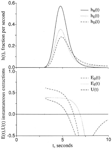
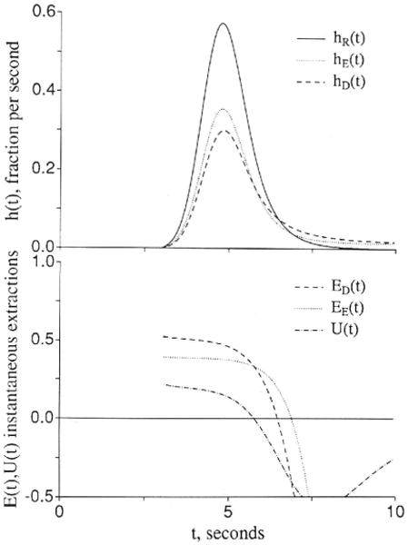
Graphs showing comparisons of outflow dilution curves [h(t)s] and apparent extractions E(t)s when an extracellular solute (subscripted E) and a test solute (subscripted D) have the same overall conductance between the plasma and interstitial fluid spaces. The input function was a lagged normal density function¹⁸ with a mean time of 2.0 seconds, relative dispersion of 0.4, and skewness of 0.9. U(t) is 1 − h_D(t)/h_E(t) and represents extraction of the test solute relative to the extracellular reference solute. Left panel: The extracellular and the endothelial permeating solutes use totally different paths. F_p = 1.0, PS_gE = 0.5, PS_gD = 0, PS_ecl = 1, PS_eca = 1, and PS_pc = 0 (ml/g)/min; ${\mathrm{V}}_{\mathrm{P}}={\mathrm{V}}_{\text{ec}}^{\prime }=0.025\text{ml}/\mathrm{g}$, and ${\mathrm{V}}_{\text{isf}}^{\prime }=0.15\text{ml}/\mathrm{g}$. (For definition of terms, refer to Figure 1.) Right panel: The aqueous cleft pathway provides for half the capillary permeability of the test solute. PS_gD = 0.25, PS_ecl = 0.5, and PS_eca = 0.5 (ml/g)/min, and other parameters are the same as in the left panel.

$$\mathrm{E}(\mathrm{t})=1-{\mathrm{h}}_{\mathrm{D}}(\mathrm{t})/{\mathrm{h}}_{\mathrm{R}}(\mathrm{t})$$

Another, proposed by Yudilevich²⁸ and called “uptake” or U(t), is obtained by comparison between the extracellular tracer dilution curve, h_E(t), and the permeant that enters cells:

$$\mathrm{U}(\mathrm{t})=1-{\mathrm{h}}_{\mathrm{D}}(\mathrm{t})/{\mathrm{h}}_{\mathrm{E}}(\mathrm{t})$$

In Figure 2, two situations are illustrated. In both, the total capillary permeability–surface area products are the same for the extracellular tracer and for the test tracer that enters and crosses endothelial cells.

For Figure 2A, the cleft is open only for the extracellular reference tracer, and the test solute passes through to the ISF only by crossing endothelial cells but with the same overall resistance between blood and ISF; thus, with PS_eca = PS_ecl for the test solute

$${\text{PS}}_{{\mathrm{g}}_{\mathrm{E}}}=0.5{\text{PS}}_{\text{ec}l}=0.5{\text{PS}}_{\text{eca}}$$

since for the test solute the overall capillary PS is 1/(1/PS_ecl+ 1/PS_eca). The solutions show that the initial extractions, the E(t)s, E_E(t) and E_D(t), differ; E_D(t) is higher than for the extracellular marker because PS_ecl is twice as high as PS_g. But this difference soon diminishes as the intraendothelial concentration rises and there is both “back diffusion” from the endothelial cell to the capillary lumen and also a gradient built up to produce flux from endothelial cell to ISF. Then E_D(t) comes closer to E_E(t) but remains dissimilar because of the difference in the timing of the backflux. Even though the late phases of backflux from ISF to plasma occur at the same rate in the two cases, the early backflux is faster because of the high PS_ecl, and the ISF concentration does not rise as high as for the extracellular reference. The result is that the tail of the curve is lower for h_D(t) whereas the early downslope is higher. [The areas of h_E(t) and h_D(t) are identical at 1.0 since there is no consumption.]

In Figure 2B, a more realistic case is presented, again with identical overall permeabilities fromplasma to ISF for the extracellular and test solutes. In this case, the cleft is open to both of the permeating solutes, but half of the capillary permeability for the test solute is assigned to the cleft and half to the endothelial cell. The difference between the two permeating solutes is diminished, as reflected by the lower U(t). The lower the ratio of PS_ecl and PS_eca to PS_g the less becomes the sensitivity to the endothelial component. The value of accurate data acquisition and the utility of the extracellular reference rise in the same instance. Clearly, the ability to estimate PS_ecl and PS_eca separately from PS_g vanishes in the absence of data on h_E(t).

Endothelial permeability

Figure 3 shows sets of responses to a dispersed input function, arranged in order of increasing openness of the capillary barrier. In Figure 3A the cleft is closed, as for brain capillaries, and the only permeation is into the endothelial cell, but not beyond, since PS_eca is zero. Increasing values of PS_ecl allow solute to enter the volume of distribution of the endothelium, which is set at 0.05 ml/g, a little larger than in the usual in vivo situation in order that the curves be easily distinguished. Increasing PS_ecl initially decreases the height of the peak of h_D(t), but then when the permeability gets so high that the endothelial luminal barrier is little hindrance, the initial extraction reaches nearly 100%. The extraction, E(t), is 1 − h_D(t)/h_R(t), and so only in the early moments is E(t) a measure of unidirectional flux and is soon thereafter reduced more and more by back diffusion or reflux from the tissue into the capillary and the effluent. In this illustration ${\mathrm{V}}_{\text{ec}}^{\prime }$, the volume of distribution for the solute in the endothelial cell, is as large as the capillary space, and opening up the cell results in delay of the efflux. At low PS_ecl the delay is expressed as a long tail, but as the permeability increases to very high values, the curve becomes more and more compact. This does not change the mean transit time for the solute, which is $({\mathrm{V}}_{\mathrm{p}}+{\mathrm{V}}_{\text{ec}}^{\prime })/{\mathrm{F}}_{\mathrm{p}}$ or V_p(1 + γ_ec)/F_p for all cases with PS_ecl>0 no matter what the form of the curve. At the highest permeability h_D(t) is high peaked and narrow and, by similarity scaling for the mean transit time, can be superimposed on the curve for zero permeability, h_R(t). This is the traveling wave case of Goresky²⁹ for flow-limited transport along the capillary-tissue unit. The interpretation is that the permeability is so high that only the flow limits the transport from the entrance to the exit. (Similar cases are shown in Figure 4.)

Figure 3.

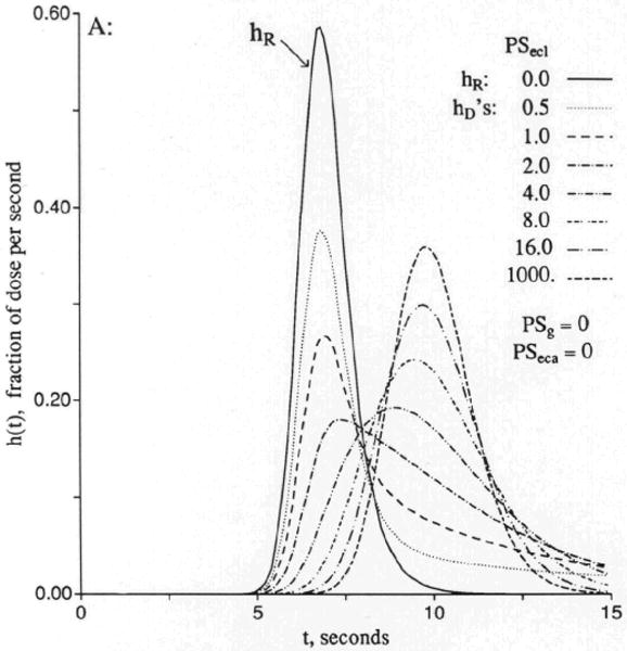
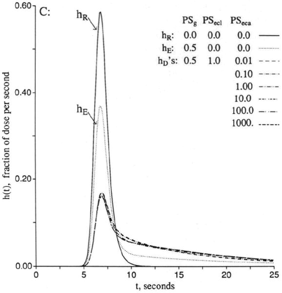
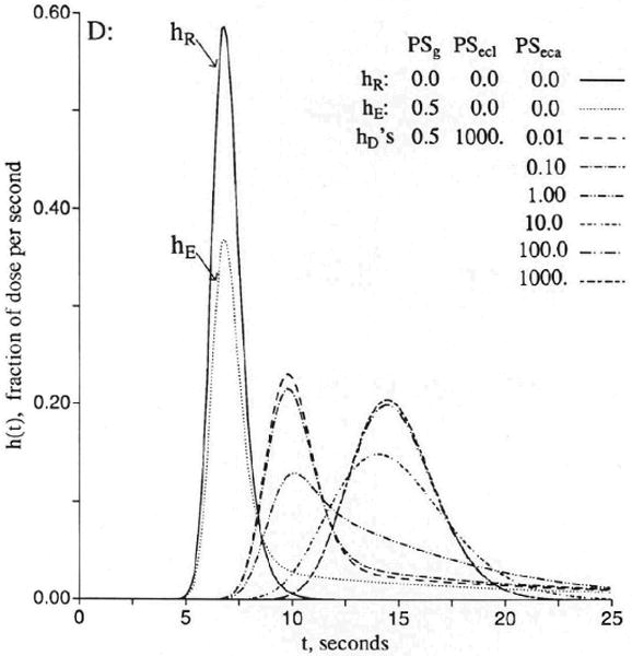
Graphs showing outflow dilution curves [h(t)s] for solute entry into three regions of the four-region capillary–endothelial cell–interstitial fluid–parenchymal cell model. h_R, intravascular reference tracer; h_D, test diffusible solute; h_E, extracellular reference tracer. For all panels, other values were F_p=1, PS_pc = 0, and all Gs = 0 (ml/g)/min and V_p = 0.05, ${\mathrm{V}}_{\text{ec}}^{\prime }=0.05$, and ${\mathrm{V}}_{\text{isf}}^{\prime }=0.08\text{ml}/\mathrm{g}$. (For definition of terms, refer to Figure 1.) Input function was a lagged normal density function with a mean of 4.0 seconds, relative dispersion of 0.20, and skewness of 0.9. Panel 3A: With the cleft permeability PS_g = 0, increasing PS_ecl gives increasingly rapid access to ${\mathrm{V}}_{\text{ec}}^{\prime }$ and, finally, flow-limited exchange at PS_ecl = 1,000. Panel 3B: With finite cleft permeability, PS_g = 0.5 (ml/g)/min, entry into and reflux from ISF creates a long tail, and a smaller fraction enters the endothelial cell. Panel 3C: With restricting barriers at both cleft and endothelial luminal surface, PS_g = 0.5 (ml/g)/min and PS_ecl = 1.0 (ml/g)/min, changing PS_eca has maximal effect at 8 and 20 seconds. Panel 3D: When PS_ecl is high, there is great sensitivity to PS_eca because, at levels equal to or higher than PS_g, it controls entry into ISF. At high values of PS_ecl and PS_eca, the transport is again flow-limited, analogous to the high PS_ecl curves in panel 3A.

Figure 4.

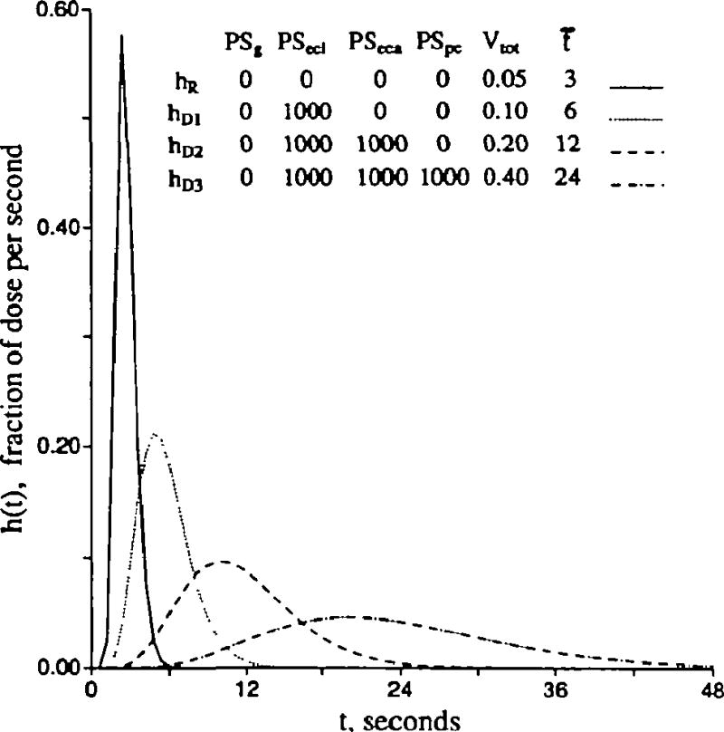
Graph showing flow-limited exchange between plasma and surrounding regions. The response h_R(t) is a vascular reference curve identical to that of Figure 3. The outflow curves [h(t)s] for the permeant represent three cases with free entry and exchange with endothelial cells only (h_D1), with endothelial cells plus interstitial fluid (h_D2), and with all three extravascular regions (h_D3). h_R is the intravascular reference tracer. The mean transit time, t̄, for each case is the total volume of distribution divided by the flow F_s = 1.0 (ml/g)/min. The volumes were V_p = 0.05, ${\mathrm{V}}_{\text{ec}}^{\prime }=0.05$, ${\mathrm{V}}_{\text{isf}}^{\prime }=0.10$, and ${\mathrm{V}}_{\text{pc}}^{\prime }=0.2\text{ml}/\mathrm{g}$. (For definition of terms, refer to Figure 1.) V_tot is the total volume accessible to solute, ml/g.

For Figure 3B, the permeability of the interendothelial cleft has been opened, PS_g = 0.5 (ml/g)/min, so that the outflow curve [h_ecf(t)] for a solute that enters only the extracellular fluid space has an initial extraction of about 39% and a long tail. For this tracer, the mean transit time is $({\mathrm{V}}_{\mathrm{p}}+{\mathrm{V}}_{\text{isf}}^{\prime })/{\mathrm{F}}_{\mathrm{p}}$. Then the permeant tracer has equal freedom to enter the ISF and can also enter the endothelial cells at a rate governed by PS_ecl as in Figure 3A. The entry into the ISF would appear to be enhanced when PS_ecl is high, and although this might seem reasonable because of the slowing of the overall transport along the unit, it is really not true. The fraction entering the ISF is no larger for the permeant, h_D(t), than for the extracellular tracer, h_ecf(t), since PS_eca = 0. The two have the same PS_g/F_p, which is independent of the volume of distribution in capillary and endothelial cell, and, therefore, the same unidirectional flux through the cleft. The greater contact time during transcapillary passage for the permeant solute that occurs with enlarging the space, ${\mathrm{V}}_{\mathrm{p}}+{\mathrm{V}}_{\text{ec}}^{\prime }$, is exactly offset by reducing the concentration gradient by the dilution in that same space, an exact cancellation. Thus, while the curve for high PS_ecl is broader, the area under the late peak above the long low tail is just the same.

In Figure 3C, the conditions are the same for the extracellular marker, with outflow curve h_ecf(t), while the value of PS_ecl is held constant at 1.0 (ml/g)/min. The curve for PS_eca = 0.001 (ml/g)/min is to be compared with the second h_D(t) of Figure 3B, that for PS_ecl=1.0. As with h_D(t) in Figure 3B, the mean transit time volume is ${\mathrm{V}}_{\mathrm{p}}+{\mathrm{V}}_{\text{ec}}^{\prime }+{\mathrm{V}}_{\text{isf}}^{\prime }$ for all of the variously shaped curves. Because entry into the endothelial cell is limited by the low value of PS_ecl, the curves do not evolve to the flow-limited form.

In Figure 3D, the conditions are the same except for setting an infinitely high value of PS_ecl. This means that when the lowest PS_eca is effectively zero, the curve of h_D(t) is flow-limited within the distribution volume ${\mathrm{V}}_{\mathrm{p}}+{\mathrm{V}}_{\text{ec}}^{\prime }$, as shown by the highest peaked of the middle curves, although the barrier for entry into the ISF through the cleft causes a long tail, which persists with slow entry across the abluminal surface of the cell. However, as that surface permeability opens up, the long tail gradually disappears, and a new peak appears around the later time $\overline{\mathrm{t}}=({\mathrm{V}}_{\mathrm{p}}+{\mathrm{V}}_{\text{ec}}^{\prime }+{\mathrm{V}}_{\text{isf}}^{\prime })/{\mathrm{F}}_{\mathrm{p}}$. In contrast to the curves for the same PS_ecas in Figure 3C, because PS_ecl is also large, the transport becomes truly flow-limited like the high PS_ecl curve of Figure 3A with the volume of distribution including everything outside the parenchymal cell.

Permeation into the parenchymal cell gives rise to similar phenomena. When PS_pc is low, entry into parenchymal cells has only a small effect on the curves shown in Figure 3. When PS_pc becomes very high, the curves are again flow-limited within the volume of distribution so that $\overline{\mathrm{t}}=({\mathrm{V}}_{\mathrm{p}}+{\mathrm{V}}_{\text{ec}}^{\prime }+{\mathrm{V}}_{\text{ISF}}^{\prime }+{\mathrm{V}}_{\text{pc}}^{\prime })/{\mathrm{F}}_{\mathrm{p}}$, as is shown in Figure 4.

Endothelial uptake and retention

Can the fate of intraendothelial solute be ascertained from the forms of outflow dilution curves? Usually, yes. In this section, we examine the distinction between uptake into an enlarging intraendothelial volume, ${\mathrm{V}}_{\text{ec}}^{\prime }$, versus intraendothelial sequestration by an irreversible first-order reaction, G_ec. ${\mathrm{V}}_{\text{ec}}^{\prime }/{\mathrm{V}}_{\text{ec}}$, a ratio of volume of distribution to true volume, greater than 1.0 results when there is either membrane transporter asymmetry (entry>efflux) or intracellular equilibrium binding to some binding site. These are indistinguishable. (Slow binding and slow release from an intracellular site is kinetically the same as slow exchange with an intracellular organelle and is not considered in this model.) Increases in either ${\mathrm{V}}_{\text{ec}}^{\prime }$ or G_ec cause diminution in reflux from the cell; this diminution lowers and narrows the peak of h_D(t). No distinction can be made when either ${\mathrm{V}}_{\text{ec}}^{\prime }$ or G_ec are high, but they can be distinguished at intermediate levels. Bassingthwaighte and Sparks³⁰ showed that, when there is transformation into a metabolite that escapes, the metabolite from endothelial cells reaches the outflow much sooner than that from parenchymal cells. Figure 5 shows contrast of the influences of uptake by binding reversibly to an intracellular site (enlarged ${\mathrm{V}}_{\text{ec}}^{\prime }$) and of uptake by consumption or unidirectional binding (due to G_ec). Representing reversible binding by enlarging ${\mathrm{V}}_{\text{ec}}^{\prime }$ allows reflux from the binding site back into the free fluid of the endothelial cell and thence to the outflow. In contrast, irreversible consumption or infinitely high affinity binding (G_ec) allows no reflux of the transformed or bound solute. At the extremes of having many binding sites or infinitely rapid consuming reactions, there is no distinction to be made between these two types of mechanisms. Distinction can be made via kinetics only when there is something to observe at the outflow, and when there is no reflux at all, the kinetics and, thus, the mechanisms must remain a mystery. However, in the midrange, differences are easily discerned.

Figure 5.

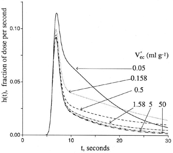
Graphs showing contrasting effects of increasing endothelial volume $({\mathrm{V}}_{\text{ec}}^{\prime })$ versus increasing intraendothelial gulosity or consumption (G_ec) on the outflow dilution curves [h(t)s]. Control conditions (upper curves in both panels) are F_p = 1, PS_g = 1, PS_ecl = 1, PS_eca = 0, PS_pc = 0, and all Gs = 0 (ml/g)/min and V_p = 0.05, ${\mathrm{V}}_{\text{ec}}^{\prime }=0.05$, and ${\mathrm{V}}_{\text{isf}}^{\prime }=0.08\text{ml}/\mathrm{g}$. (For definition of terms, refer to Figure 1; input function is the same as in Figure 3.) Left panel: Enlarging ${\mathrm{V}}_{\text{ec}}^{\prime }$ by successive multiplication by 10^1/2 from 0.05 to 50 ml/g has no effect on the early upslope, causes some reduction in peak height, and has its main effect on reduction of return flux in the early downslope portion. Right panel: G_ec increased by successive 10-fold increases from 0.001 to 100 (ml/g)/min reduces backflux in both the early and late times after the peak.

In Figure 5, left panel, the upper curve gives the reference situation, a ${\mathrm{V}}_{\text{ec}}^{\prime }$ of 0.05 ml/g and PS_ecl = 1.0 (ml/g)/min, which is very similar to the fourth curve of Figure 3B. By increasing the intraendothelial volume of distribution by factors of 10^1/2, one obtains a set of curves of which the lowest (that with the highest ${\mathrm{V}}_{\text{ec}}^{\prime }$) is equivalent to an infinite volume of distribution and no reflux from the cell. The intermediate curves are dramatically lower than the control curve at 10 seconds and give a measure of how much reflux has been occurring with the smaller volume of distribution. Note that enlarging ${\mathrm{V}}_{\text{ec}}^{\prime }$ reduces the peak height by about 20%; this finding gives evidence that the Crone-Renkin expression PS = − F log_e(1 − E) must underestimate PS when calculated from E_peak. With the highest ${\mathrm{V}}_{\text{ec}}^{\prime }$, the PS so calculated should represent the sum of PS_g and PS_ecl. The early upslope of h_D(t) is relatively uninfluenced; if there were no heterogeneities in flows or capillary transit times, the estimates of PS by this Equation from the upslope extraction would be accurate.

The tails of the curves in Figure 5, left panel, also show the effects of an enlarged volume of distribution. With 3.2- and 10-fold increases in ${\mathrm{V}}_{\text{ec}}^{\prime }$, the extraction, increased by 40–60% at around the tenth second, diminishes rapidly as reflux occurs from the binding sites to the intracellular space and to the effluent. This is the range of expected effects for tracer solute when the nontracer mother solute is in equilibrium with the binding site and the solute concentration is 1/3–1/10; of the dissociation constant for the binding. If we suppose that there is a reference tracer with similar permeability, but no binding, so that it has a dilution curve of the shape of the uppermost curve, then the early higher extraction, the later reflux, and the fact that the curves for ${\mathrm{V}}_{\text{ec}}^{\prime }=0.158$ and ${\mathrm{V}}_{\text{ec}}^{\prime }=0.5$ cross over that for ${\mathrm{V}}_{\text{ec}}^{\prime }=0.05$ ml/g indicate an increase in the volume of distribution by reversible binding.

Figure 5, right panel, shows the effects of consumption, transformation, or irreversible binding. A transformation, with release of the product into the cytoplasm may not be recognized unless the outflow samples are analyzed to distinguish substrate from product; ordinarily this means distinguishing them by chemical or physical techniques since isotope counting methods won't distinguish chemical forms. The interesting point relevant to distinguishing the irreversible binding from the reversible binding is that the forms of the curves for the nonextreme conditions in the left and right panels of Figure 5 are very differently shaped. Only when the volume or reaction effects are very small or very large is it difficult to distinguish the processes.

Intraendothelial binding versus surface binding

When the transmembrane transport is saturable, this linear model can still be used to obtain estimates of the Michaelis constant, K_m, and maximum velocity, V_max, for the nonlinear transporter. As Malcorps et al²⁷ and Catravas et al³² describe, the strategy is to obtain a set of estimates of PS at different concentrations of the substrate, from zero to well above the K_m. In this section, we tackle the problem of how to estimate the concentration dependency of functional volumes of distribution for solutes that bind to specific sites. To illustrate the strategy, we concentrate on the simplest cases, namely, those binding either with instantaneous equilibration at the endothelial luminal surface or those binding so slowly that slow on-and-off kinetics are discernible.

Here we consider how to distinguish between three somewhat analogous but different situations: 1) cell entry with dilution and delay that normally occurs for substances that do not bind, 2) no cell entry, but equilibrium binding to a surface site on the luminal plasmalemmal surface, and 3) a variant on case 2, but with nonequilibrium conditions, slow adsorption and dissociation from a surface binding site or receptor. Figure 6, left panel, shows a set of solutions for equilibrium binding to surface sites in contact with the plasma; these are precisely equivalent to increasing the volume of distribution in the plasma space. The logic and the equations are similar to those used by Safford and Bassingthwaighte³² for the volume of distribution of calcium augmenting a diffusion space. The method of detection and quantitation depends on performing simultaneous dilution curves for an intravascular reference solute and for the solute that is transiently bound. (Albumin may not be the best intravascular reference because it has been found to have binding sites on the capillary endothelial surface in the heart.^33,34) If there were no intracapillary dispersion, then the effect on the curve for the bound solute would be a simple shift to the right with a spread proportional to the shift (again as above), which is the effect of a flow-limited distribution through an instantly available but enlarged volume of distribution.²⁹ If intravascular dispersion is the same for the reference and the binding tracers, then this simple similarity of form will be observed.

Figure 6.

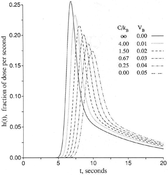
Graphs showing receptor binding: effects of rapid equilibrative surface binding versus slow exchange with a surface receptor site in parallel with entry into endothelial cells. Left panel: An equilibrating surface binding site acts simply as an enlarged volume of distribution. Because binding and unbinding are “infinitely” rapid there is no limitation to exchange with the additional space, and the outflow curve shows a flow-limited form similar to that for which there is no binding. h(t) is the normalized outflow dilution curve. Parameters to represent surface binding are PS_B = 1,000 (ml/g)/min, V_p = 0.05 ml/g, and V_B = 0−0.05 ml/g; others are the same as in right panel. Right panel: Slow exchange with a receptor on the endothelial luminal surface is analogous, for tracer, with first-order exchange with another region. In these curves the tracer exchanges with both the endothelial cell and with a binding site. Both are first-order exchanges, applicable to a situation with constant concentrations of nontracer mother solute; even the transport or binding processes may be concentration dependent. The conditions for this figure are F_p = 1.0, PS_ecl = 1.0, PS_eca = 0, PS_g = 0, G_ec = 0, and PS_B = 1.0 (ml/g)/min, while ${\mathrm{V}}_{\text{ec}}^{\prime }=0.08\text{ml}/\mathrm{g}$ and V_B varied from 0 to 0.05 ml/g. (For definition of terms, refer to Figure 1; input function is the same as in Figure 3; k_B and V_B are defined with Equation 52.)

The additional space available to the binding solute is dependent on the number of binding sites and the concentration of the nontracer form of the binding solute in steady state, which governs the level of occupancy of the sites. For a site whose total concentration is B_T moles per liter capillary volume and whose molar equilibrium dissociation constant is k_B, the volume of distribution is V_p plus the binding space, V_B, which is

$${\mathrm{V}}_{\mathrm{B}}=\frac{{\mathrm{B}}_{\mathrm{T}}{\mathrm{V}}_{\mathrm{P}}}{\mathrm{C}+k_{\mathrm{B}}}$$ (52)

where C is the molar solute concentration. The expression suggests an experimental approach for the estimation of the space V_B by changing the concentration C over a wide range around the k_B; when C = k_B, the sites are half saturated, and the value of V_B is half of what it would be at its maximum when there is no nontracer substrate present. Thus, the maximum volume is B_T V_p/k_B. Under the condition of equilibrium binding, the presence of a receptor only enlarges a volume of distribution and is exactly equivalent to the flow-limited case. A series of experiments at different flows and at constant concentration of the nontracer mother solute will then show a constant difference in mean transit time volume between an inert intravascular marker and the substrate participating in the binding. To determine the k_B, one needs to perform a series of indicator dilution curves at different nontracer steady-state solute concentrations, estimate V_B from each, and then obtain B_T and k_B by fitting the V_B versus C relation with Equation 52. Note that this analysis uses only linear modeling to get V_B, and the nonlinear modeling of Equation 52 follows simply thereafter.

Distinction is more difficult between impeded entry into the cell, dilution and exit, and the combination of slow binding by a receptor, transient retention, and release. In one sense we can regard this four-region model as being suited to either situation since the basic equations can be reexpressed for a surface receptor without endothelial cell space, with only a few limitations. Consider a case in which there is no entry into ISF or parenchymal cells but there is exchange with both a receptor and the endothelial cell cytoplasm. The simplest case (no exchange between receptor and cell cytoplasm) is shown in Figure 6, right panel. The intravascular reference curve h_R(t) is not shown because it is identical to those shown in Figure 3. The values for ${\mathrm{V}}_{\text{ec}}^{\prime }$ and PS_ecl are held constant, and PS_eca and PS_g = 0, so there is no entry into ISF. With increasing V_B, uptake and retention onto the receptor site lowers the peak of the curve and prolongs the tail. In this situation, the set of curves is exactly the same as if PS_g = 1.0 (ml/g)/min and ${\mathrm{V}}_{\text{ISF}}^{\prime }$ were varied from 0 to 0.05 ml/g. Slow exchange with membrane-bound receptor can be expressed on the basis that nontracer mother substance has equilibrated but tracer has not. The parameters are as follows: k_on, rate of substrate binding to receptor, cubic centimeters per millimole per second; k_off, rate of substrate release from receptor, per second; k_B, equilibrium dissociation constant, millimoles per cubic centimeter (k_B = k_off/k_on = R · C/RC); C, concentration of substrate, molar or millimoles per cubic centimeter; V, regional volume of distribution for substrate, milliliters per gram; R_T, total receptor concentration in the volume containing the substrate, molar or millimoles per cubic centimeter; and RC, R, concentrations of complexed and free receptor in the volume, molar or millimoles per cubic centimeter.

At equilibrium, RC and R, are given by

$$\mathrm{R}=\frac{k_{\mathrm{B}}{\mathrm{R}}_{\mathrm{T}}}{\mathrm{C}+k_{\mathrm{B}}}$$ (53)

$$\text{RC}={\mathrm{R}}_{\mathrm{T}}-\mathrm{R}=\frac{\mathrm{C}\cdot {\mathrm{R}}_{\mathrm{T}}}{\mathrm{C}+k_{\mathrm{B}}}$$ (54)

Concentration of the total receptors accessible from this space = R_TV mmol/g, [(mmole/cm³)×(cm³/g)]. If R, RC, and R_T are strictly on the membrane surface, with surface area S cm²/g, then R_TV/S is the density per unit membrane surface area, mol/cm² [(mmol/g)/(cm²/g)].

The equations for exchange between receptor and substrate free in the volume are

$$\mathrm{V}\frac{\text{dC}}{\text{dt}}=-{\text{PS}}_{\mathrm{B}}\cdot {\mathrm{C}+\text{PS}}_{-\mathrm{B}}\cdot \text{RC}$$ (55)

$$\mathrm{V}\frac{\text{dRC}}{\text{dt}}={\text{PS}}_{\mathrm{B}}\cdot \mathrm{C}-{\text{PS}}_{-\mathrm{B}}\cdot \text{RC}$$ (56)

$${\mathrm{R}}_{\mathrm{T}}=\mathrm{R}+\text{RC}$$ (57)

$$\frac{\text{dRC}}{\text{dt}}=-\frac{\text{dR}}{\text{dt}}$$ (58)

where PS_B and PS_−B are clearances into or back from the bound state and where

$$\frac{{\text{PS}}_{\mathrm{B}}}{\mathrm{V}}=k_{\text{on}}\cdot \mathrm{R}=k_{\text{on}}\cdot \frac{k_{\mathrm{B}}}{\mathrm{C}+k_{\mathrm{B}}}\cdot {\mathrm{R}}_{\mathrm{T}}$$ (59)

with the units, cm³/(mmol·s⁻¹)×(mmol/cm³) or s^−l, which gives the units of PS_B to be k_on · R · V (ml/g)/s. Similarly, PS_−B = k_off · V (ml/g)/s.

With RC=C·R_T/(C+k_B), the binding process buffers the free-solute concentration and raises the effective volume of distribution:

$$\begin{array}{l}\mathrm{V}\prime /\mathrm{V}=[\text{RC}+\mathrm{C}]/\mathrm{C}\\ =[\mathrm{C}\cdot {\mathrm{R}}_{\mathrm{T}}/(\mathrm{C}+k_{\mathrm{B}})+\mathrm{C}]/\mathrm{C}=1+\frac{{\mathrm{R}}_{\mathrm{T}}}{\mathrm{C}+k_{\mathrm{B}}}\end{array}$$ (60)

When R_T is small or C> >k_B, then V′/V is little more than 1. This is an appropriate expression consonant with the principle that volumes of distribution are observable by equilibrium experiments. The strategy is similar to that of Goresky et al.³⁵ Further, ${\mathrm{V}}_{\mathrm{p}}^{\prime }$ is now seen as equal to V_p + V_B, where V_B = V_pR_T/(C + k_B) as in Equation 52. As with equilibrium binding, the experimental approach is to perform tracer experiments in the presence of steady background levels of nontracer mother solute. The indicator dilution data can take forms similar to the left panel of Figure 6 if PS_B and PS _−B are high compared with F_p and can take forms similar to the right panel if PS_B and PS_−B are of the same order as F_p.

These same strategies can be applied to binding in the interstitium and in parenchymal cells. Slow on-and-off kinetics requires the use of an additional region to represent the binding site volume of distribution. Thus, although we could use the present four-region model to represent luminal surface receptors instead of an endothelial cell, slow binding to other surfaces when all four regions are accessible to the solute will require additional regions to be added to the model. In essence, each would be an additional equation added to Equations 1–4. In the numerical scheme, this would be handled by enlarging the 4 × 4 matrix in Equation 43. Depending on the connectivity of the regions, more off-diagonal terms might be required. This formulation can be made quite general, as shown by Schwab³⁶; thus, the current model may be viewed as a simple four-region implementation of more complex models that could be put into practice.

The problem of the small endothelial volume

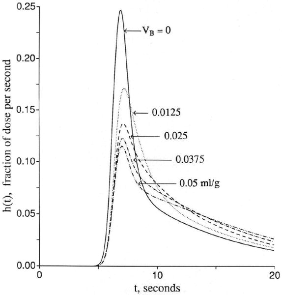
The anatomic volume of endothelial cells is somewhat less than the capillary blood volume; for the heart, the endothelial thickness is as small as 0.2 μm but probably averages near 0.4 μm when the thick nuclear region is included. Given a capillary surface area of 500 cm²/g, the volume would be 500×0.4×10⁻⁴ = 0.02 ml/g or about half the capillary volume. If intraendothelial binding and transformation are insignificant, can PS_ecl and ${\mathrm{V}}_{\text{ec}}^{\prime }$ be estimated from the dilution curves? A test case is shown in Figure 7 with ${\mathrm{V}}_{\text{ec}}^{\prime }/{\mathrm{V}}_{\mathrm{p}}$ or γ_ec = 0.5; four solutions, all with PS_eca = 0, were obtained at different PS_ecl. The results show a distinct difference between h_D(t) when PS_ecl>0 compared with the case when PS_ecl = 0. But the differences are subtle enough that, to estimate ${\mathrm{V}}_{\text{ec}}^{\prime }$ in the presence of permeation via the cleft into the interstitium, a well-matching extracellular reference marker should be used simultaneously. When h_E(t), the extracellular reference, and h_D(t), the permeant, have the same PS_g and ${\mathrm{V}}_{\text{isf}}^{\prime }$, then ${\mathrm{V}}_{\text{ec}}^{\prime }$ should be measurable in experiments with high time resolution sampling (>1 sample/second) and 2–3% accuracy in h_D(t). Although such a case as this with PS_ecl>0 and PS_eca = 0 is not very likely, this is a worst case situation because PS_ecl is much easier to measure if there is intraendothelial binding giving a larger ${\mathrm{V}}_{\text{ec}}^{\prime }$, if there is intraendothelial consumption as products have similar sensitivity (G_ec>0), or if there is permeation through the abluminal surface (PS_eca>0). All three situations reduce the rapidity of reflux from endothelial cell to plasma.

Figure 7.

Graph showing influence of luminal endothelial permeability (PS_ecl) on outflow dilution curve [h(t)] when the endothelial volume is small and antiluminal endothelial permeability is zero. h_R, intravascular reference tracer. Other parameters are V_p = 0.05, ${\mathrm{V}}_{\text{ec}}^{\prime }=0.025$, ${\mathrm{V}}_{\text{isf}}^{\prime }=0.2$, and ${\mathrm{V}}_{\text{pc}}^{\prime }=0.5\text{ml}/\mathrm{g}$; PS_g = 0.5, PS_eca = 0, and PS_pc = 1.0 (ml/g)/min; F_p = 1 (ml/g)/min. (For definition of terms, refer to Figure 1.)

Accuracy in estimating ${\mathrm{V}}_{\text{ec}}^{\prime }$ is less when both PS_ecl and PS_eca are high since the solute then passes through the endothelial cell and is diluted (or reacted upon) in ISF or parenchymal cells. Here the need for an equivalent extracellular reference tracer is even more critical, and with it endothelial parameters are more clearly identifiable. Sensitivity analysis, presented below, gives specific information on the influence of endothelial and other parameters on the outflow data.

Influences of Interstitium and Parenchymal Cells

The effects of events in ISF and parenchymal cells on the outflow dilution curves is somewhat blunted and blurred by endothelial events. Outflow dilution analyses are dependent on isolating the influences of these system components on the tails of curves because the material takes time to reach and return from ISF and cells. At low rates of entry into ISF very little can be learned about the parenchymal cell unless, of course, direct measurements can be made of cell contents or there is evidence of solute transformation such as the emergence of a reaction product into the outflow. Fortunately, for many solutes the values of PS_g are high enough that interstitial and cellular events are readily assessable.

There are certain situations in which it is essential to obtain other evidence in addition to dilution curves. When there is endothelial uptake, then the effects of removal of substrate by interstitial consumption or irreversible binding in the ISF or to a cell surface are indistinguishable, mathematically as well as experimentally, from irreversible uptake by parenchymal cells. Reversible binding to an interstitial site may be indistinguishable from a bidirectional flux into a parenchymal volume of distribution; that is, if V_Bisf equals ${\mathrm{V}}_{\text{pc}}^{\prime }$ and the rate of binding PS_B equals PS_pc, the effects on the outflow are identical. The distinction must be made experimentally by exploring over a concentration range below and above the apparent K_m for the binding site.

The effect of uptake into parenchymal cells with a large volume of distribution is identical to consumption of tracer within the interstitial space, which is evident from the parallel terms PS_pc×C_isf and G_isf×C_isf in Equation 3. Parenchymal cell consumption has a similar effect, but it is delayed. Endothelial uptake from ISF has a similar effect, as suggested by the term P_eca×C_isf in Equation 3, if the cell volume is large or if G_ec is also high and PS_ecl is near zero. All of these mechanisms retard or prevent reflux of tracer from the parenchymal cell or interstitial space back to the vascular outflow. Because of the similarity of these influences, it is apparent that there will be some difficulties in estimating parameters accurately. Distinction between interstitial consumption and the combination of parenchymal cell uptake and consumption is impossible from early data, as seen in Figure 8. An outflow detection technique cannot distinguish untransformed from transformed tracer residual in the tissue. Histochemical or other techniques that distinguish substrate from product might be used to detect the differences among substrates, intracellular products, and products formed in the interstitium.

Figure 8.

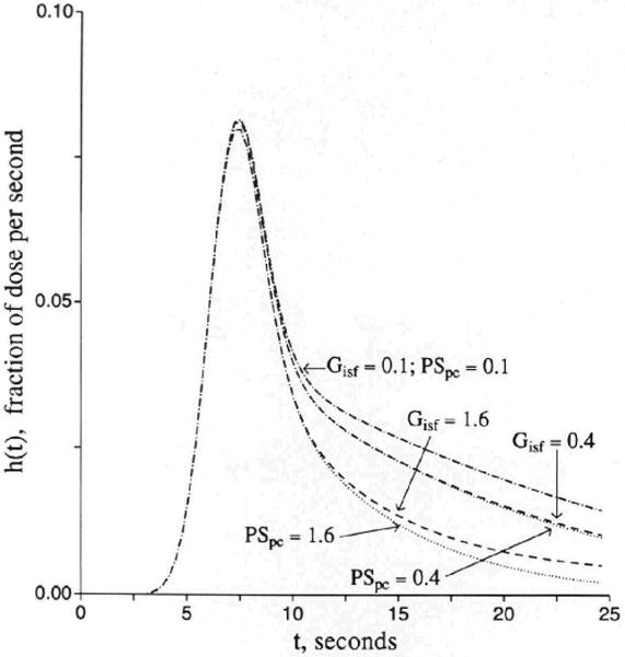
Graph showing influences of interstitial consumption and cellular uptake on outflow dilution curve [h(t)]. Other parameters are the same as for Figure 3.

Goresky and colleagues^35,37 developed models for a saturable metabolic process, but they did not include endothelial cells. Our model will substitute for theirs exactly when the concentrations are well below the K_m of the reaction, covering their cases with two, one, or zero barriers.

Sensitivity Analysis as an Aid to Testing Parameter Identifiability

Sensitivity functions give an indication of the relative sensitivities of the model solution to its parameters for any particular parameter set. Independence of parameters from one another is demonstrated when there are clear-cut differences in shapes of sensitivity functions. Formally stated, parameters are independent when no two have sensitivity functions superimposable by scaling or inverting by multiplying by a negative scalar. Parameters appearing as products have similar sensitivity functions whereas those appearing as quotients have scaled mirror image sensitivity functions.^38,39 Similarity in sensitivity functions is useful in making one aware of interdependence that may be functional and not mathematical. When sensitivity functions show small differences relative to the noise in observed data functions, this indicates that certain parameters cannot be distinguished. Sometimes reporting the sum or ratio of two parameters is useful. For these cylindrical axisymmetric convection-diffusion models the following general statements can be made: 1) Values for parameters for parts of the system distant from the vascular space can be discerned with less accuracy than those close to the vascular region. 2) When conductances for barriers near the vascular space are high, the sensitivity to parameters farther away increases. 3) Conductivity for flux into a large distant region is difficult or impossible to distinguish from consumption or permanent binding in the region next in proximity to the vascular system; for example, interstitial consumption and permeation into a large parenchymal cell volume are not distinguishable unless the data set is long enough for return flux to occur from the parenchymal cell to the vascular effluent. 4) Residue function experiments in which washout is recorded over a long period of time give better information on the deeper parts of the system than can be obtained by outflow indicator dilution experiments in which the tails of h_D(t) are very low. The residue types of experiments (by external detection of tracer) also give a different weighting on the information than do outflow techniques although identical models can be used for analysis of the two types of signals. 5) In systems with this many free parameters, it is critically important to constrain parameter values by virtue of other information sets. This is best done by use of multiple tracer techniques in which the other information sets are provided by data obtained simultaneously from tracers whose transport is constrained in known fashions (e.g., no consumption, no entry into cells, or no escape from the vascular space). Data on steady-state volumes of distribution from experiments done in very similar circumstances is very useful in limiting the range of possible values. 6) Axial diffusion plays a role in governing the shapes of the late tails of the curve as well as in influencing the early upslope and fitting of the front end of indicator dilution curves. Axial dispersion, either by using the Poisson flow models or the plug flow models with dispersiveness intravascularly, is useful in refined fitting of the initial portions of the concentration and extraction curves. Since model solutions are speeded up by not using axial diffusion expressions, the strategy for obtaining best fits of models to data may include leaving out axial diffusion until final phases of the fitting process. The diffusion coefficients should be constrained by estimates obtained elsewhere and by using anatomic knowledge for effective lengths.

Examining the sensitivity functions is a direct means of evaluating the questions relating to whether or not a particular experiment can yield definitive information. Sensitivity functions are defined as the rate of change of the model function over its whole time course with respect to an incremental change in the parameter value with all other parameter values remaining constant. Thus, a particular sensitivity function, for example for PS_ecl, is dependent on the specific conditions of the other parameters as well as on the form of the model itself. The formal expression for the sensitivity function S_i(P̰,t) for the i^th parameter depends on the parameter vector P̰ and time:

$${\mathrm{S}}_{\mathrm{i}}\left(\underset{\sim }{\mathbf{\text{P}}},\mathrm{t}\right)=\partial \mathrm{h}(\mathrm{t})/\partial {\mathrm{p}}_{\mathrm{i}}$$ (61)

where p_i is the i^th parameter. There is a sensitivity curve for each parameter. (These S_i(P,t)s are not related to the step function, S(T), in Equation 24.) But if there were not two solutes, extracellular and permeant, with similar PS_gs, then PS_g and PS_ecl would be difficult to distinguish with low resolution data, which would make identification difficult, as foreseen by Haselton et al⁴⁰ and by Cobelli and DiStefano in their more formal treatment of compartmental modeling.⁴¹

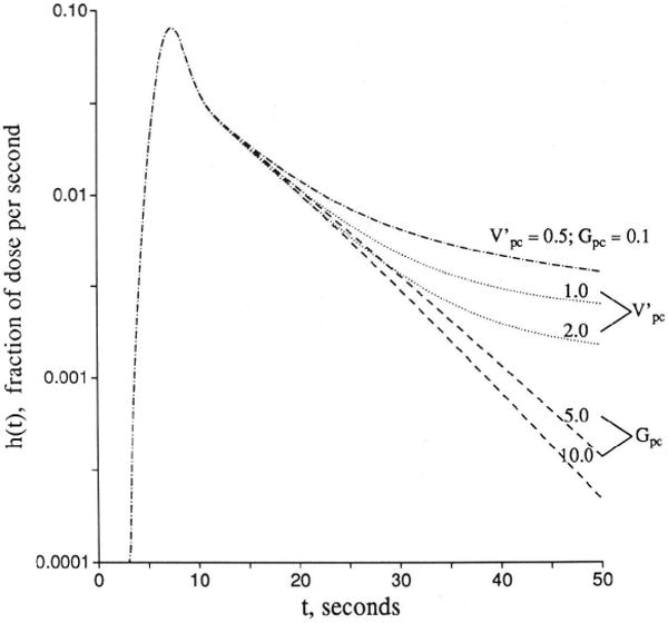
Sensitivity functions are shown in Figure 9 for two typical situations. For conservative parameters, PS and V, the sensitivity functions are always biphasic. They are negative initially because increasing the parameter results in more loss from plasma or less backflux. They are positive later because whatever tracer escaped from the vascular space must return later. For consuming parameters G, the sensitivity functions are unimodal, always negative. The first situation (left panel) is for moderate values of PS_g and PS_ecl, giving about a 50% extraction, in which the sensitivity to the parameters for cleft and endothelial permeation is high. None of the S(t)s have either similar or mirror image shapes, which is formal evidence that the parameters are mathematically identifiable. Note that not only are the forms of S_i(P,t) for PS_g and PS_ecl different but also that there is a substantial separation between those for PS_ecl and PS_eca. The right panel is for values of PS_g, PS_ecl, and PS_eca that are about 50% greater than those in the left panel; the sensitivities to these three parameters are less, but the sensitivity to the parameters governing the exchanges with the parts of the system farther from the capillary are increased for PS_pc and ${\mathrm{V}}_{\text{pc}}^{\prime }$. At very low rates of permeation of the capillary barrier, sensitivity to these latter parameters becomes small, but not zero, since the long retention that occurs with entry into the parenchymal cell strongly influences the tail. This is a situation where the residue detection methodology is better since the amount held in the tissue is directly measured. As a vehicle for exploring the design of experiments, sensitivity functions are extremely useful, not just for determining that parameters are distinguishable but also for defining where the effort needs to be made in the data acquisition (e.g., how many samples? at which times? with what tolerable measurement error?).

Figure 9.

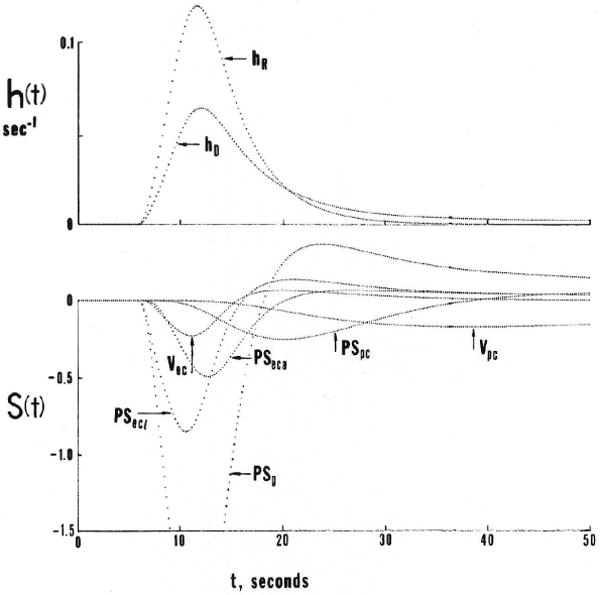
Graphs showing sensitivity functions for the four-region capillary-endothelial-interstitial cell model. Upper curves show the model responses to a dispersed input function [h(t)] for both a vascular reference solute (h_R) and a permeating solute h_D. Lower panels show sensitivity function [S(t)] for several parameters. Left panel: PS_g and PS_ecl are relatively low. Right panel: With higher PS_g, the sensitivities to more distant events, governed by PS_pc and V_pc, are increased. (For definition of terms, refer to Figure 1.)

Axial Diffusion or Dispersion

For brief recordings of outflow indicator dilution curves (those sampled for less than a minute) axial diffusion in the plasma has an important effect on the initial upslopes, but diffusion in the extravascular regions has little effect. Intratissue diffusion has an important influence on the later stages of washout whenever there is partial flow limitation to washout. The effect of increasing D_isf or D_pc is the lowering of the fractional escape rate for retained tracer, which is the rate of tracer washout as a fraction of that retained in the capillary-tissue units. This is explained as follows: there is always a tendency for tracer to accumulate at the most downstream end of the capillary-tissue unit. This is because tracer refluxing from tissue into plasma nearer the upstream end has a chance to reescape from plasma into tissue at points further downstream. The accumulation downstream sets up a gradient in the tissue with the highest concentration at the downstream end of the extravascular regions. (This is analogous to, but opposite in gradients from, the region of minimum oxygen concentration when there is consumption.) This is also the position from which the probability of escape from the organ, the fractional escape rate from the tissue, is the highest since there is almost no possibility of reuptake from plasma into tissue when the tracer flux into the capillary is so very close to the venous outflow. The effect of axial diffusion is to diminish the axial intratissue concentration gradient by giving net diffusional flux from downstream toward upstream and by opposing the accumulation. The effects of downstream convection in the plasma and partial reescape into tissue thus become balanced exactly by net upstream diffusion and reflux into the capillary at more upstream locations than would occur without axial diffusion.

The balancing of these opposing effects is seen in the stabilization of the shape of the tail of the outflow curve; it becomes monoexponential, which is to say, the fractional escape rate becomes constant. To an observer who cannot see within the tissue with high spatial resolution, this would appear to support the idea that the capillary-tissue unit behaves as a mixing chamber; it really means that the gradients in the spatial concentration profiles have stabilized in position. After the stabilizing balancing of convective and diffusive influences, the concentrations at all points decay exponentially with a rate constant equal to the fractional escape rate for the whole unit. An example of the spatial profile that sets up at later times is shown in Figure 10.

Figure 10.

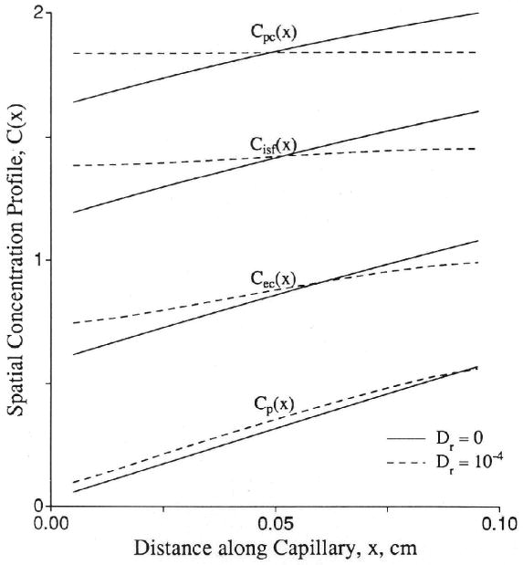
Graph showing spatial concentration (C) profiles in a capillary-tissue exchange unit at t = 200 seconds. At this time, the concentration in each location relative to the peak concentration in the downstream corner remains at a constant ratio. The parameters were F_p = PS_ecl = PS_eca = PS_pc = 1.0 (ml/g)/min; PS_g = 0; V_p = 0.05, ${\mathrm{V}}_{\text{ec}}^{\prime }=0.025$, ${\mathrm{V}}_{\text{isf}}^{\prime }=0.2$, and ${\mathrm{V}}_{\text{pc}}^{\prime }=0.5\text{ml}/\mathrm{g}$. (For definition of terms, refer to Figure 1.) Control axial diffusion (D_r) = 0 (solid lines); all D_r = 10⁻⁴ cm²/sec (dashed lines). At t = 200 seconds, the residue function is 0.044 for the control case and 0.045 for the test case. The fractional escape rates η(t) at t = 200 sec were 0.00771/sec for D_r = 0 and 0.00755/sec for D_r = 10⁻⁴ cm²/sec.

The analytic solution given in Equation 34 does not account for axial diffusion. This shortcoming creates two problems in fitting data. The first problem occurs during the early upslope of high resolution indicator dilution curves where intravascular axial dispersion, combining with the simultaneous permeation across the capillary wall, influences the shape of the outflow curve for the nonextractcd fraction of a permeating tracer, h_D(t), differently than it does the curve for the completely unextracted reference tracer, h_R(t). The result is seen most readily in the shape of the instantaneous extraction, E(t) = 1 − h_D/h_R, as shown in Figure 11, or in plots of the log ratio ln[h_D(t)/h_R(t)]. [Extravascular diffusion has no influence on this part of the curve at low values of PS_g and PS_ecl, and the effect is still negligible with D_isf at 2 × 10⁻⁵ cm²/sec (a high value achieved only for tracer water diffusion in aqueous solution) with PS/F_p as high as 4.0 and D_isf × V_isf/(F_p × L²) = 0.2, a maximal value.] When the intraplasma diffusion coefficient, D_PR, for the reference intravascular tracer equals that for the permeant, D_PD, there is relatively more spreading of h_R(t) than h_D(t) with the result that E(t) is initially lower than predicted by the Crone-Renkin expression E = 1 − exp(−PS/F_p) and rises to a later peak. This is what is usually seen with high temporal resolution dilution curves; the probable physical situation is that the effective intracapillary dispersion is dominated more by local nonlaminar convection than by molecular diffusion so that albumin and a small permeant have similar D_p. In simple laminar flow this phenomenon would be opposed by a Taylor diffusion effect in which more rapid radial intracapillary diffusion of the smaller solute across the velocity gradients would tend to inhibit the axial spread of the permeant more than that of the reference tracer. The curves obtained with D_PD < D_PR in the left panel of Figure 11 would present a predominantly Taylor diffusion regime; a smaller D_PD than D_PR in a plug flow regime has the same effect as a higher radial diffusion coefficient for the permeant than for the intravascular reference solute has in a parabolic flow regime.

Figure 11.

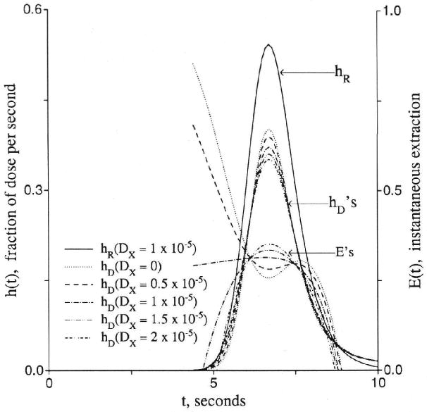
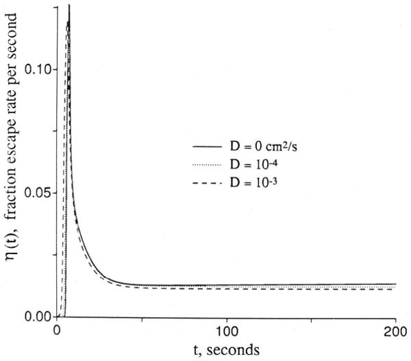
Graphs showing effects of axial diffusion (D or D_x) on the shape of outflow dilution curve [h(t)], instantaneous extraction [E(t)], and fractional escape rate [η(t)]. Upper panel: Curves for intravascular reference tracer (h_R), test diffusible solute (h_D), and E(t) at different ratios of intraplasma diffusion coefficients. Lower panel: Fractional escape rates η(t) = h(t)/R(t) for the permeating tracer at different diffusion coefficients. All permeability–surface area products are 1.0 (ml/g)/min.

The second problem in using analytic solutions lacking axial diffusion is in the washout phase because, with D_r = 0 in all regions, the fractional escape rises with time and h(t) decreases increasingly rapidly and deviates downward from monoexponential form. We have never observed dilution curves with increasing fractional escape rates at late times, even when followed down to 10⁻⁴ times the peak value. Flow heterogeneity tends to make the tail of composite residue or outflow curves concave upward on a semilog plot when the individual components are all monoexponential, but a finite D_r helps to fit the curves without exaggerating the flow heterogeneity.

An example of the strategy used in manual parameter adjustment to fit the model to outflow dilution curves after bolus injection into the inflow begins by fitting the intravascular reference curve with a multicapillary model with flow heterogeneity from the measured regional flow distribution and with PS, set to zero. The extracellular reference solute is then fitted by use of the same model as for intravascular transport, but allowing D_P, PS_g, and ${\mathrm{V}}_{\text{ISF}}^{\prime }$ to be adjusted to fit the data particularly around the appearance time and upslope of h_E(t); thus it is initially the same for h_R(t) and h_E(t), the intravascular and extracellular solutes. Then, given that h_R(t) is well fitted, D_PE is adjusted to improve the fitting of h_E(t) and its early extraction curve. The next step of the fitting is to refine the estimates of ${\mathrm{V}}_{\text{ISF}}^{\prime }$ by adjusting it and D_ISFE for the extracellular tracer. Values of less than 10⁻⁵ cm²/sec usually suffice to offset the rise in fractional escape rate at late times for individual units and give the appropriate curvature to the composite multicapillary outflow dilution curve model.

Discussion

The model has extensive applicability in studies of solutes bound to, transported into, or metabolized by endothelial cells. The use of the high resolution multiple tracer indicator dilution methodology allows evaluation of kinetic events in a fashion that is not possible with cultured or isolated endothelial cells. The key is using the intact organ's vascular system to run fluid past the surface of the cells at high velocity and to collect the effluent with minimal retarding volume between the cells and the sample collector. Collecting venous outflow samples by direct catheterization or by using isolated organs serves the purpose admirably.

To illustrate, we choose two example situations in which transport into or across endothelial cells is important, the extraction of tracer adenosine and tracer fatty acid. The details of the experiments are presented elsewhere, as are evaluations and implications of the parameter estimates.

The studies of adenosine transport in guinea pig hearts used [¹³¹I]albumin as the intravascular reference, h_R(t), [³H]AraH as the extracellular reference, h_E(t), and [¹⁴C]adenosine as the permeant, h_D(t). The organ was the isolated heart, perfused with Krebs-Ringer bicarbonate buffer at a flow of 5.2 (ml/g)/min at 50 mm Hg pressure. The outflow was collected in sequential tubes preloaded with reagents to stop adenosine deamination, as described by Wangler et al.⁴² The distribution of regional myocardial blood flows was estimated from microsphere distributions to have a relative dispersion of about 50% in 50-mg pieces. The distribution was considered to be adequately described by a five-element histogram; this defined the flow distribution w(f) as the finite distribution w_i(f_i) to be used in Equation 5. The input to the model was deconvoluted from the observed h_R(t) and served as the input for all three tracers, as described by Kuikka et al.⁵ Parameters of the model solution were adjusted to fit h_E(t) to the AraH curve, thereby defining PS_g and ${\mathrm{V}}_{\text{ISF}}^{\prime }$. It was assumed that there was no consumption in isf (G_ISF = 0), and the adenosine curve was then fitted with an optimizing parameter adjustment routine. The results are shown in Figure 12 for one set of curves. The confidence limits on the estimates of PS_eca are quite wide; this variation and its implications are considered in detail by Wangler et al.⁴²

Figure 12.

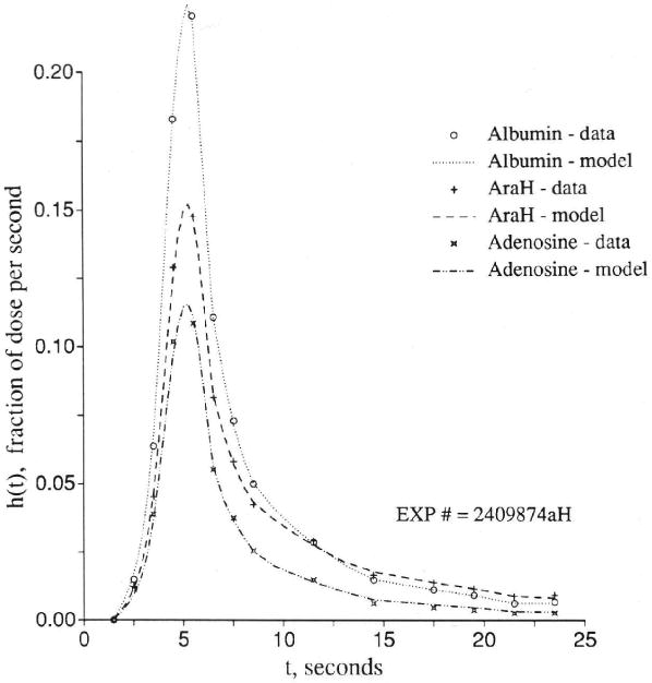
Graph showing adenosine, arabinofuranosyl hypoxanthine (AraH), and albumin outflow dilution curve [h(t)] in an isolated perfused guinea pig heart. F_p = 5.2 (ml/g)/min. Model-to-data coefficients of variation were 5.0% for albumin curve, 3.1% for sucrose, and 5.7% for adenosine. Flow heterogeneity was accounted for by using five capillary tissue units in parallel with a relative dispersion of 50%. ${\mathrm{V}}_{\text{isf}}^{\prime }=0.19\text{ml}/\mathrm{g}$ for AraH and adenosine. The cleft PS_g was 1.34 (ml/g)/min for AraH and adenosine. Other adenosine parameters were PS_ecl= 2.25, PS_eca = 20, G_ec = 30, PS_pc = 6, and G_pc = 10 (ml/g)/min, and ${\mathrm{V}}_{\text{pc}}^{\prime }=0.62$, V_p = 0.04, and ${\mathrm{V}}_{\text{ec}}^{\prime }=0.02\text{ml}/\mathrm{g}$ (For definition of terms, refer to Figure 1.)

In a similar study, fatty acid, [¹⁴C]palmitate, was injected into the inflow of isolated perfused rabbit hearts with sucrose and albumin as reference extracellular and intravascular solutes.³⁴ This is a more peculiar case since palmitate is so tightly bound to intravascular albumin that only negligible amounts traverse the clefts and PS_g was effectively zero. The transport across the endothelial barrier is saturable at higher concentrations of the albumin–fatty acid complex, but in this solution we merely find the best fitting PS_ecl. The further assumption that G_ec is zero and all the consumption is in the myocyte sets the conditions so that PS_eca and PS_pc are adjusted by use of the value of ${\mathrm{V}}_{\text{isf}}^{\prime }$ obtained for sucrose. The result is shown in Figure 13.

Figure 13.

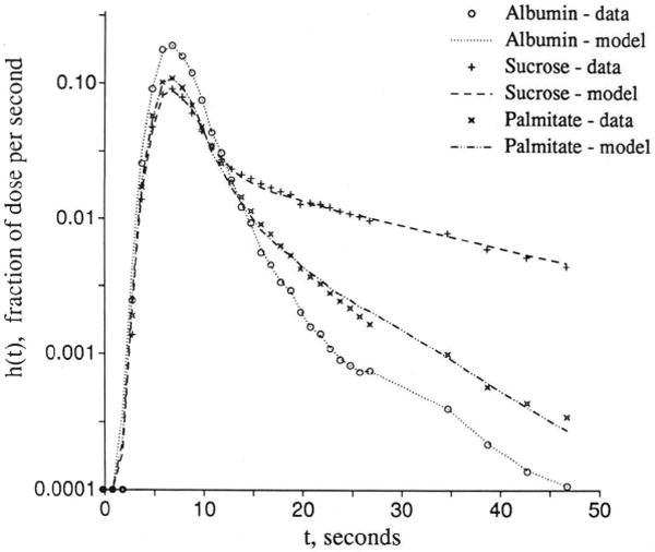
Graph showing palmitate uptake in the isolated rabbit heart. Outflow dilution curves [h(t)s] for albumin, sucrose, and [¹⁴C]palmitate were obtained with Krebs-Ringer perfusate containing 0.4 mM albumin and 0.4 mM total palmitate at F_p = 1.6 (ml/g)/min. Model-to-data coefficients of variation were 9.5% for albumin curve, 6.4% for sucrose, and 7.3% for adenosine. Flow heterogeneity was accounted for by five paths with a relative dispersion of 50%. ${\mathrm{V}}_{\text{isf}}^{\prime }=0.36\text{ml}/\mathrm{g}$ for sucrose. The cleft PS_g was 1.31 (ml/g)/min for sucrose and 0 for palmitate. Other palmitate parameters were PS_ecl = 1.02, PS_eca = 1.4, G_ec = 0, PS_pc = 2.7, and G_pc = 8.1 (ml/g)/min and ${\mathrm{V}}_{\text{pc}}^{\prime }=4.3$, V_p = 0.04, and ${\mathrm{V}}_{\text{ec}}^{\prime }=0.02\text{ml}/\mathrm{g}$ (G. van der Vusse and S. Little, unpublished data). (For definition of terms, refer to Figure 1.)

Conclusion

The model is demonstrated to be applicable to examples of important situations in which the role of the endothelial cell is prominent and also in which parenchymal cells are involved. The analytic solution, available only for the situation in which axial diffusion is negligible, is too cumbersome for practice, and because axial diffusion is deemed important, our numerical solutions are more general, as well as being faster to compute. By using carefully chosen sets of reference solutes, including an extracellular one matched in molecular weight with the solute of interest, constraints can be put on parameters related to intravascular and extracellular events. These constraints make possible the estimation of endothelial and parenchymal cell parameters with a better approximation of endothelial parameters than of parenchymal cell parameters.

Appendix

Estimation of Ratios of Endothelial Cell to Parenchymal Cell Deposition of Infused Tracer Adenosine

A steady state is obtained after about the first 2 minutes of a constant infusion. Then simplified equations give a fairly good approximation to the relative concentrations in each region of a four-region capillary-tissue exchange model. These same equations may be augmented to include storage in forms other than the primary substrate; for adenosine, storage as adenine nucleotide is the main consideration. The equations do not provide for reflux of tracer adenosine from intracellular pools, such as the adenine nucleotides or S-adenosyl-l-homocysteine (SAH), and are therefore regarded as being suitable whenever such a pool is so large that there is time to reach a pseudo–steady-state before measurable reflux occurs or whenever the pool is so small that equilibration with it occurs rapidly. The ATP pool is the former type; SAH is the latter.

The steady-state form of the differential equations sets the derivatives to zero:

$$\begin{array}{l}0=-{\mathrm{F}}_p\mathrm{L}\frac{{\text{dC}}_{\mathrm{p}}}{\text{dx}}-{\text{PS}}_g({\mathrm{C}}_p-{\mathrm{C}}_{\mathit{\text{isf}}})-{\text{PS}}_{\mathit{\text{ecl}}}({\mathrm{C}}_p-{\mathrm{C}}_{\mathit{\text{ec}}})-{\mathrm{G}}_p{\mathrm{C}}_p\\ 0=-{\text{PS}}_{\text{ec}l}({\mathrm{C}}_{\text{ec}}-{\mathrm{C}}_{\mathrm{p}})-{\text{PS}}_{\text{eca}}({\mathrm{C}}_{\text{ec}}-{\mathrm{C}}_{\text{isf}})-{\mathrm{G}}_{\text{ec}}{\mathrm{C}}_{\text{ec}}\\ 0=-{\text{PS}}_{\mathrm{g}}({\mathrm{C}}_{\text{isf}}-{\mathrm{C}}_{\mathrm{p}})-{\text{PS}}_{\text{eca}}({\mathrm{C}}_{\text{isf}}-{\mathrm{C}}_{\text{ec}})-{\text{PS}}_{\text{pc}}({\mathrm{C}}_{\text{isf}}-{\mathrm{C}}_{\text{pc}})-{\mathrm{G}}_{\text{isf}}{\mathrm{C}}_{\text{isf}}\\ 0=-{\text{PS}}_{\text{pc}}({\mathrm{C}}_{\text{pc}}-{\mathrm{C}}_{\text{isf}})-{\mathrm{G}}_{\text{pc}}{\mathrm{C}}_{\text{pc}}\end{array}$$

Now, for efficiency in expression, we put

$$\begin{array}{c}{\mathrm{C}}_{\mathrm{p}}=\mathrm{U}{\mathrm{C}}_{\text{ec}}=\mathrm{V},{\mathrm{C}}_{\text{isf}}=\mathrm{W}{\mathrm{C}}_{\text{pc}}=\mathrm{Z}\\ {\mathrm{F}}_{\mathrm{p}}\mathrm{L}=\alpha {\text{PS}}_{\mathrm{g}}=k_1{\text{PS}}_{\text{ec}l}=k_2{\text{PS}}_{\text{eca}}=k_4{\text{PS}}_{\text{pc}}=k_6\\ {\mathrm{G}}_{\mathrm{p}}=k_3{\mathrm{G}}_{\text{ec}}=k_5{\mathrm{G}}_{\text{isf}}=k_7{\mathrm{G}}_{\text{pc}}=k_8\end{array}$$

The steady-state equations are now expressed:

$$0=-\alpha \frac{\text{dU}}{\text{dx}}-k_1\left(\mathrm{U}-\mathrm{W}\right)-k_2\left(\mathrm{U}-\mathrm{V}\right)-k_3\mathrm{U}$$ (A1)

$$0=-k_2\left(\mathrm{V}-\mathrm{U}\right)-k_4\left(\mathrm{V}-\mathrm{W}\right)-k_5\mathrm{V}$$ (A2)

$$0=-k_1(\mathrm{W}-\mathrm{U})-k_4(\mathrm{W}-\mathrm{V})-k_6(\mathrm{W}-\mathrm{Z})-k_7\mathrm{W}$$ (A3)

$$0=-k_6(\mathrm{Z}-\mathrm{W})-k_8\mathrm{Z}$$ (A4)

For further efficiency, groups of coefficients are defined:

$$\begin{array}{l}\text{Let}{\mathrm{B}}_1=k_2+k_4+k_5\\ {\mathrm{B}}_2=k_6+k_8\\ {\mathrm{B}}_3=k_1+k_4+k_6+k_7\\ \mathrm{D}={\mathrm{B}}_1\left({\mathrm{B}}_2{\mathrm{B}}_3-k_6^2\right)-k_4^2{\mathrm{B}}_2\end{array}$$

Using these algebraic manipulations of Equations A2–A4 allows reexpression to show the concentrations in the extravascular regions as ratios to the plasma concentration, U:

$$\begin{array}{c}\mathrm{V}=\frac{k_2\mathrm{D}+\left(k_1{\mathrm{B}}_1+k_2{k}_4\right){\mathrm{B}}_2{k}_4}{{\mathrm{B}}_1\mathrm{D}}\mathrm{U}=\frac{\left(k_2{\mathrm{B}}_3+k_1{k}_4\right){\mathrm{B}}_2-k_2{k}_6^2}{\mathrm{D}}\mathrm{U}\\ \mathrm{W}=\frac{\left(k_1{\mathrm{B}}_1+k_2{k}_4\right){\mathrm{B}}_2}{\mathrm{D}}\mathrm{U}\\ \mathrm{Z}=\frac{\left(k_1{\mathrm{B}}_1+k_2{k}_4\right)k_6}{\mathrm{D}}\mathrm{U}\end{array}$$

By substituting V and W into Equation A1, we can put Equation A1 into general form when there is no production of tracer adenosine:

$$\alpha \frac{\text{dU}}{\text{dx}}+\text{MU}=0$$ (A5)

where:

$$\mathrm{M}=k_1+k_2+k_3-\frac{k_1^2{\mathrm{B}}_1{\mathrm{B}}_2+2k_1{k}_2{k}_4{\mathrm{B}}_2+k_2^2{\mathrm{B}}_2{\mathrm{B}}_3-k_2^2{k}_6^2}{\mathrm{D}}$$

This has a first-order exponential solution:

$${\mathrm{C}}_{\mathrm{p}}(\mathrm{x})=\mathrm{U}={\mathrm{C}}_{\mathrm{a}}{\mathrm{e}}^{\frac{-\text{Mx}}{\alpha }}={\mathrm{C}}_{\mathrm{a}}{\mathrm{e}}^{\frac{-\text{Mx}}{\text{FL}}}$$ (A6)

and at x = 0, C_p = the inflow concentration C_a, and at x = L, C_p(L) = C_aexp(−M/F). The average concentrations in each region are:

$$\begin{array}{l}{\overline{\mathrm{C}}}_{\mathrm{p}}=\overline{\mathrm{U}}=\frac{1}{\mathrm{L}}{\mathrm{C}}_{\mathrm{a}}{{\int }_0^{\mathrm{L}}\mathrm{e}}^{\frac{-\text{MX}}{\alpha }}\text{dx}\\ =\frac{{\mathrm{C}}_{\mathrm{a}}}{\mathrm{L}}(-\frac{\alpha }{\mathrm{M}})\left({\mathrm{e}}^{-\text{MF}}-1\right)\\ =\frac{{\mathrm{C}}_{\mathrm{a}}\mathrm{F}}{\mathrm{M}}(1-{\mathrm{e}}^{-\text{MF}})\end{array}$$ (A7)

$${\overline{\mathrm{C}}}_{\text{ec}}=\overline{\mathrm{V}}=\frac{\left(k_2{\mathrm{B}}_3+k_1{k}_4\right){\mathrm{B}}_2-k_2{k}_6^2}{\mathrm{D}}{\overline{\mathrm{C}}}_{\mathrm{p}}$$ (A8)

$$\begin{array}{l}{\overline{\mathrm{C}}}_{\text{isf}}=\overline{\mathrm{W}}=\frac{\left(k_1{\mathrm{B}}_1+k_2{k}_4\right)}{\mathrm{D}}{\mathrm{B}}_2\frac{{\mathrm{C}}_{\mathrm{a}}\mathrm{F}}{\mathrm{M}}\left(1-e^{-\mathrm{M}/\mathrm{F}}\right)\\ =\frac{\left(k_1{\mathrm{B}}_1+k_2{k}_4\right){\mathrm{B}}_2}{\mathrm{D}}{\overline{\mathrm{C}}}_{\mathrm{p}}\end{array}$$ (A9)

$${\overline{\mathrm{C}}}_{\text{pc}}=\overline{\mathrm{Z}}=\frac{\left(k_1{\mathrm{B}}_1+k_2{k}_4\right)k_6}{\mathrm{D}}{\overline{\mathrm{C}}}_{\mathrm{p}}$$ (A10)

This allows prediction of the ratio of free intracellular concentrations of adenosine in endothelial cells compared with myocytes but does not account for tracer trapped as ATP or SAH:

$$\frac{{\overline{\mathrm{C}}}_{\text{ec}}}{{\overline{\mathrm{C}}}_{\text{pc}}}=\frac{\left(k_2{\mathrm{B}}_3+k_1{k}_4\right){\mathrm{B}}_2-k_2{k}_6^2}{{\mathrm{B}}_1{k}_6\left(k_1{\mathrm{B}}_1+k_2{k}_4\right)}$$ (A11)

References

- 1.Rose CP, Goresky CA, Bach GG. The capillary and sarcolemmal barriers in the heart: An exploration of labeled water permeability. Circ Res. 1977;41:515–533. doi: 10.1161/01.res.41.4.515. [DOI] [PubMed] [Google Scholar]
- 2.Perl W, Chinard FP. A convection-diffusion model of indicator transport through an organ. Circ Res. 1968;22:273–298. doi: 10.1161/01.res.22.2.273. [DOI] [PubMed] [Google Scholar]
- 3.Bassingthwaighte JB, Yipintsoi BT, Knopp TJ. Diffusional arteriovenous shunting in the heart. Microvasc Res. 1984;28:233–253. doi: 10.1016/0026-2862(84)90020-7. [DOI] [PMC free article] [PubMed] [Google Scholar]
- 4.Bassingthwaighte JB. A concurrent flow model for extraction during transcapillary passage. Circ Res. 1974;35:483–503. doi: 10.1161/01.res.35.3.483. [DOI] [PMC free article] [PubMed] [Google Scholar]
- 5.Kuikka J, Levin M, Bassingthwaighte JB. Multiple tracer dilution estimates of D- and 2-deoxy-D-glucose uptake by the heart. Am J Physiol. 1986;250(Heart Circ Physiol 19):H29–H42. doi: 10.1152/ajpheart.1986.250.1.H29. [DOI] [PMC free article] [PubMed] [Google Scholar]
- 6.Bassingthwaighte JB, Chan IS, Wang CY. Computationally efficient algorithms for capillary convection-permeation-diffusion models for blood-tissue exchange. Ann Biomed Eng. doi: 10.1007/BF02368613. in press. [DOI] [PubMed] [Google Scholar]
- 7.Rickaby DA, Linehan JH, Bronikowski TA, Dawson CA. Kinetics of serotonin uptake in the dog lung. J Appl Physiol. 1981;51:405–414. doi: 10.1152/jappl.1981.51.2.405. [DOI] [PubMed] [Google Scholar]
- 8.Linehan JH, Dawson CA. A kinetic model of prostaglandin metabolism in the lung. J Appl Physiol. 1979;47:404–411. doi: 10.1152/jappl.1979.47.2.404. [DOI] [PubMed] [Google Scholar]
- 9.Renkin EM. Transport of potassium-42 from blood to tissue in isolated mammalian skeletal muscles. Am J Physiol. 1959;197:1205–1210. doi: 10.1152/ajplegacy.1959.197.6.1205. [DOI] [PubMed] [Google Scholar]
- 10.Crone C. The permeability of capillaries in various organs as determined by the use of the ‘indicator diffusion’ method. Acta Physiol Scand. 1963;58:292–305. doi: 10.1111/j.1748-1716.1963.tb02652.x. [DOI] [PubMed] [Google Scholar]
- 11.Linehan JH, Bronikowski TA, Dawson CA. Kinetics of uptake and metabolism by endothelial cell from indicator dilution data. Ann Biomed Eng. 1987;15:201–215. doi: 10.1007/BF02364055. [DOI] [PubMed] [Google Scholar]
- 12.Bassingthwaighte JB, Noodleman L, van der Vusse G, Little SE, Glatz JFC, Reneman RS. Albumin-fatty acid-endothelial membrane interactions and fatty acid transport in the heart (abstract) Fed Proc. 1987;46:686. [Google Scholar]
- 13.Rose CP, Goresky CA. Vasomotor control of capillary transit time heterogeneity in the canine coronary circulation. Circ Res. 1976;39:541–554. doi: 10.1161/01.res.39.4.541. [DOI] [PubMed] [Google Scholar]
- 14.Bronikowski TA, Linehan JH, Dawson CA. A mathematical analysis of the influence of perfusion heterogeneity on indicator extraction. Math Biosci. 1980;52:27–51. [Google Scholar]
- 15.Bassingthwaighte JB, Goresky CA. Modeling in the analysis of solute and water exchange in the microvasculature. In: Renkin EM, Michel CC, editors. Handbook of Physiology, Section 2: The Cardiovascular System, Volume IV, Part 1. Bethesda, Md: American Physiological Society; 1984. pp. 549–626. [Google Scholar]
- 16.Bass L, Robinson PJ. Effects of capillary heterogeneity on rates of steady uptake of substances by the intact liver. Microvasc Res. 1981;22:43–57. doi: 10.1016/0026-2862(81)90110-2. [DOI] [PubMed] [Google Scholar]
- 17.Bassingthwaighte JB, Dobbs WA, Yipintsoi T. Heterogeneity of myocardial blood flow. In: Maseri A, editor. Myocardial Blood Flow in Man: Methods and Significance in Coronary Disease. Torino, Italy: Minerva Medica; 1972. pp. 197–205. [Google Scholar]
- 18.Bassingthwaighte JB. Plasma indicator dispersion in arteries of the human leg. Circ Res. 1966;19:332–346. doi: 10.1161/01.res.19.2.332. [DOI] [PMC free article] [PubMed] [Google Scholar]
- 19.Olsen SP, Crone C. Electrical resistance of muscle capillary endothelium. Biophys J. 1983;42:31–41. doi: 10.1016/S0006-3495(83)84366-5. [DOI] [PMC free article] [PubMed] [Google Scholar]
- 20.Levin M, Kuikka J, Bassingthwaighte JB. Sensitivity analysis in optimization of time-distributed parameters for a coronary circulation model. Med Prog Technol. 1980;7:119–124. [PMC free article] [PubMed] [Google Scholar]
- 21.Sangren WC, Sheppard CW. A mathematical derivation of the exchange of a labeled substance between a liquid flowing in a vessel and an external compartment. Bull Math Biophys. 1953;15:387–394. [Google Scholar]
- 22.Oberhettinger F. Tables of Bessel Transforms. Berlin: Springer-Verlag; 1972. [Google Scholar]
- 23.Bateman H. Tables of Integral Transforms. II. New York: McGraw-Hill Book Co; 1954. [Google Scholar]
- 24.Bassingthwaighte JB, Lenhoff AM, Stephenson JL. A sliding-element algorithm for rapid resolution of spatially distributed convection-permeation models (abstract) Biophys J. 1984;45:175a. [Google Scholar]
- 25.Cody WJ, Fraser W, Hart JF. Rational Chebyshev approximation using linear equations. Numer Math. 1968;12:242–251. [Google Scholar]
- 26.Lenhoff AM, Lightfoot EN. The effects of axial diffusion and permeability barriers on the transient response of tissue cylinders. II. Solutions in time domain. J Theor Biol. 1984;106:207–238. doi: 10.1016/0022-5193(84)90020-1. [DOI] [PubMed] [Google Scholar]
- 27.Malcorps CM, Dawson CA, Linehan JH, Bronikowski TA, Rickaby DA, Herman AG, Will JA. Lung serotonin uptake kinetics from indicator-dilution and constant-infusion methods. J Appl Physiol. 1984;57:720–730. doi: 10.1152/jappl.1984.57.3.720. [DOI] [PubMed] [Google Scholar]
- 28.Syrota A, Girault M, Pocidalo JJ, Yudilevich DL. Endothelial uptake of amino acids, sugars, lipids, and prostaglandins in rat lung. Am J Physiol. 1982;243:C20–C26. doi: 10.1152/ajpcell.1982.243.1.C20. [DOI] [PubMed] [Google Scholar]
- 29.Goresky CA. A linear method for determining liver sinusoidal and extravascular volumes. Am J Physiol. 1963;204:626–640. doi: 10.1152/ajplegacy.1963.204.4.626. [DOI] [PubMed] [Google Scholar]
- 30.Bassingthwaighte JB, Sparks HV. Indicator dilution estimation of capillary endothelial transport. Annu Rev Physiol. 1986;48:321–334. doi: 10.1146/annurev.ph.48.030186.001541. [DOI] [PMC free article] [PubMed] [Google Scholar]
- 31.Catravas JD, Bassingthwaighte JB, Sparks HV., Jr . Adenosine transport and uptake by cardiac and pulmonary endothelial cells. In: Ryan US, editor. Endothelial Cells. I. Boca Raton, Fla: CRC Press; 1988. pp. 65–84. [Google Scholar]
- 32.Safford RE, Bassingthwaighte JB. Calcium diffusion in transient and steady states in muscle. Biophys J. 1977;20:113–136. doi: 10.1016/S0006-3495(77)85539-2. [DOI] [PMC free article] [PubMed] [Google Scholar]
- 33.Ghitescu L, Fixman A, Simionescu M, Sitnionescu N. Specific binding sites for albumin restricted to plasmalemmal vesicles of continuous capillary endothelium: Receptor-mediated transcytosis. J Cell Biol. 1986;102:1304–1311. doi: 10.1083/jcb.102.4.1304. [DOI] [PMC free article] [PubMed] [Google Scholar]
- 34.Little SE, van der Vusse GJ, Bassingthwaighte JB. Estimation of transcapillary transport of palmitate by the multiple indicator dilution technique (abstract) Fed Proc. 1986;45:613. [Google Scholar]
- 35.Goresky CA, Bach GG, Rose CP. Effects of saturating metabolic uptake on space profiles and tracer kinetics. Am J Physiol. 1983;244:G215–G232. doi: 10.1152/ajpgi.1983.244.2.G215. [DOI] [PubMed] [Google Scholar]
- 36.Schwab AJ. Extension of the theory of the multiple-indicator dilution technique to metabolic systems with an arbitrary number of rate constants. Math Biosci. 1984;71:57–79. [Google Scholar]
- 37.Goresky CA, Bach GG, Nadeau BE. On the uptake of materials by the intact liver: The transport and net removal of galactose. J Clin Invest. 1973;52:991–1009. doi: 10.1172/JCI107300. [DOI] [PMC free article] [PubMed] [Google Scholar]
- 38.Beck JV, Arnold KJ. Parameter Estimation in Engineering and Science. New York: John Wiley & Sons, Inc; 1977. [Google Scholar]
- 39.Frank PM. Introduction to System Sensitivity Theory. New York: Academic Press, Inc; 1978. [Google Scholar]
- 40.Haselton FR, Roselli RJ, Parker RE, Harris TR. An effective-diffusivity model of pulmonary capillary exchange: General theory, limiting cases, and sensitivity analysis. Math Biosci. 1984;70:237–263. [Google Scholar]
- 41.Cobelli C, DiStefano JJ., III Parameter and structural identifiability concepts and ambiguities: A critical review and analysis. Am J Physiol. 1980;239:R7–R24. doi: 10.1152/ajpregu.1980.239.1.R7. [DOI] [PubMed] [Google Scholar]
- 42.Wangler RD, Gorman MW, Wang CY, DeWitt DF, Chan IS, Bassingthwaighte JB, Sparks HV. Transcapillary adenosine transport and interstitial adenosine concentration in guinea pig hearts. Am J Physiol. 1989;257(Heart Circ Physiol 26):H89–H106. doi: 10.1152/ajpheart.1989.257.1.H89. [DOI] [PMC free article] [PubMed] [Google Scholar]