Linking crystallographic model and data quality

Abstract

In macromolecular X-ray crystallography, refinement R values measure the agreement between observed and calculated data. Analogously, R_merge values reporting on the agreement between multiple measurements of a given reflection are used to assess data quality. We here show that despite their widespread use, R_merge values are poorly suited for determining the high resolution limit, and that current standard protocols discard much useful data. We introduce a statistic that estimates the correlation of an observed dataset with the underlying (not measurable) true signal; this quantity, CC*, provides a single statistically-valid guide for deciding which data are useful. CC* also can be used to assess model and data quality on the same scale and this reveals when data quality is limiting model improvement.

Accurately determined protein structures provide insight into how biology functions at the molecular level and also guide the development of new drugs and protein-based nanomachines and technologies. The large majority of protein structures are determined by X-ray crystallography, where measured diffraction data is used to derive a molecular model. Surprisingly, despite decades of methodology development, the question of how to select the resolution cutoff of a crystallographic dataset is still controversial and the link between the quality of the data and the quality of the derived molecular model is poorly understood. Here, we describe a statistical guide that allows assessment of the resolution limit that will optimize model quality.

The measured data in X-ray crystallography are the intensities of reflections, and these yield structure factor amplitudes each with unique h, k, l indices which define the lattice planes. The standard indicator for assessing the agreement of a refined model with the data is the crystallographic R value, defined as

$$R=\frac{\sum _{\mathit{hkl}}\mid F_{\mathit{obs}}\left(\mathit{hkl}\right)-F_{\mathit{calc}}\left(\mathit{hkl}\right)\mid }{\sum _{\mathit{hkl}}{F}_{\mathit{obs}}\left(\mathit{hkl}\right)}$$ (1)

with F_obs(hkl) and F_calc(hkl) being the observed and calculated structure factor amplitudes, respectively. R is 0.0 for perfect agreement with the data, and R is near 0.59 for a random model (1) . Because R can be made arbitrarily low for models having sufficient parameters to overfit the data, Brünger (2) introduced R_free as a cross-validated R based on a small subset of reflections not used during refinement. The R for the larger “working” set of reflections is then referred to as R_work.

Crystallographic data quality is commonly assessed by an analogous indicator R_merge (originally [3] R_sym), which measures the spread of n independent measurements of the intensity of a reflection, I_i(hkl), around their average, $\stackrel{‒}{\mathrm{I}}\left(\mathit{hkl}\right)$:

$$R_{\text{merge}}=\frac{\sum _{\mathit{hkl}}\sum _{i=1}^n\mid I_i\left(\mathit{hkl}\right)-\stackrel{‒}{I}\left(\mathit{hkl}\right)\mid }{\sum _{\mathit{hkl}}\sum _{i=1}^n{I}_i\left(\mathit{hkl}\right)}$$ (2)

In 1997, it was discovered that because I_i(hkl) influence $\stackrel{‒}{\mathrm{I}}\left(\mathit{hkl}\right)$, the R_merge definition must be adjusted by a factor of $\sqrt[]{\frac{n}{n-1}}$ to give values that are independent of the multiplicity (4). The multiplicity-corrected version, called R_meas, reliably reports on the consistency of the individual measurements. A further variant, R_pim (5), reports on the expected precision of $\stackrel{‒}{\mathrm{I}}\left(\mathit{hkl}\right)$ and is lower by a factor of $\frac{1}{\sqrt[]{n}}$ factor compared to R_meas. Because the strength of diffraction decreases with resolution, a high-resolution cutoff is applied to discard data considered so weak that their inclusion might degrade the quality of the resulting model. Data are typically truncated at a resolution before the R_merge (or R_meas) value exceeds ~0.6 - 0.8 and before the empirical signal-to-noise ratio, $<\stackrel{‒}{\mathrm{I}}∕\sigma \left(\stackrel{‒}{\mathrm{I}}\right)>$, drops below ~2.0 (6) (Figure S1). The uncertainty associated with these criteria is illustrated by a recent review that concluded “an appropriate choice of resolution cutoff is difficult and sometimes seems to be performed mainly to satisfy referees” (6).

That these criteria result in high resolution cutoffs that are too conservative is illustrated here using an example dataset (EXP) collected for a cysteine-bound complex of cysteine dioxygenase (CDO); the EXP data has about 15-fold weaker intensity than the data originally used to determine the structure at 1.42 Å resolution (PDB 3ELN; R_work/R_free=0.135/0.177) (7, 8). Standardized model refinements starting with a 1.5 Å resolution unliganded CDO structure (PDB code 2B5H (9)) were carried out against the EXP data for a series of high resolution cutoffs between 2.0 and 1.42 Å resolution (Table S1). As R value comparisons are only meaningful if calculated at the same resolution, paired refinements done with adjacent resolution limits were evaluated using R_work and R_free values calculated at the poorer resolution limit. Improvement is indicated by drops in R_free or increases in R_work at the same R_free (meaning the model is less overfit). This analysis revealed that every step of added data improved the resulting model (Figure 1). Consistent with this, difference Fourier maps show a similar trend in signal versus resolution (Figure S2), and geometric parameters of the resulting models improve with resolution (Table S2).

Figure 1.

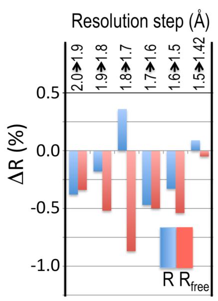
Higher resolution data, even if weak, improves refinement behaviour. For each incremental step of resolution from X->Y (top legend), the pair of bars gives the changes in overall R_work (blue) and R_free (red) for the model refined at resolution Y with respect to those for the model refined at resolution X, with both R values calculated at resolution X. The first pair of bars shows that R_work and R_free dropped 0.38 and 0.34% upon isotropic refinement, respectively, when the refinement resolution limit was extended from 2.0 to 1.9 Å; the other pairs of bars show the improvement upon anisotropic refinement.

The proven value of the data out to 1.42 Å resolution contrasts strongly with the R_meas and $<\stackrel{‒}{\mathrm{I}}∕\sigma \left(\stackrel{‒}{\mathrm{I}}\right)>$ values at that resolution (> 4.0 and ~ 0.3, respectively; Figure 2), which are far beyond the limits currently associated with useful data. Applying the typical standards described above, this dataset would have been truncated at ~1.8 Å resolution, halving the number of unique reflections in the dataset (Table S1) and yielding a worse model.

Figure 2.

Data quality R values behave differently than those from crystallographic refinement, and useful data extend well beyond what standard cutoff criteria would suggest. R_meas (squares) and R_pim (circles) are compared with R_work (blue) and R_free (red) from 1.42 Å resolution refinements against the EXP dataset. $<\stackrel{‒}{\mathrm{I}}∕\sigma \left(\stackrel{‒}{\mathrm{I}}\right)>$ (grey X) is also plotted. Inset is a close-up of the plot beyond 2 Å resolution.

It is striking to observe the different behavior at high resolution of the crystallographic versus the data-quality R values, with the one remaining below 0.40 and the other diverging toward infinity (Figure 2). Consideration of the R_merge formula rationalizes this divergence, as the denominator (the average net intensity) approaches zero at high resolution while the numerator becomes dominated by background noise and is essentially constant. Thus, despite their similar names and mathematical definitions, data-quality R values are not comparable to R values from model refinement, and there is no valid basis for the commonly applied criterion that data are not useful beyond a resolution where R_meas (or R_merge or R_pim) rises above ~0.6. As suggested by Wang (10), $<\stackrel{‒}{\mathrm{I}}∕\sigma \left(\stackrel{‒}{\mathrm{I}}\right)>$ at a much lower level than generally recommended could be used to define the cutoff, but this has the problem that $\sigma \left(\stackrel{‒}{\mathrm{I}}\right)$ values can be misestimated (6, 11).

With current standards not serving as reliable guides for selecting a high resolution cutoff, we investigated the use of the Pearson correlation coefficient (CC) (12) as a parameter that could potentially assess both data accuracy and the agreement of model and data on a common scale. Pearson’s CC is already used in crystallography, in that a CC value of 0.3 between independent measurements of anomalous signals has become the recommended criterion for selecting the high-resolution cutoff of the data to be used for defining the locations of the anomalous scatterers (13). Following a procedure suggested earlier (4), we divided the unmerged EXP data into two parts, each containing a random half of the measurements of each unique reflection. Then, the CC was calculated between the average intensities of each subset. This quantity, denoted CC_1/2, is near 1.0 at low resolution and drops to near 0.1 at high resolution (Figure 3). According to the Student’s t-test (12), the CC_1/2 of 0.09 for the ~2100 reflection pairs in the highest resolution bin is significantly different from zero (P = 2*10⁻⁵).

Figure 3.

Signal as a function of resolution as measured by correlation coefficients. Plotted as a function of resolution for the EXP data is CC_1/2 (diamonds) and the CC for a comparison with the 3ELN reference dataset (triangles). $<\stackrel{‒}{\mathrm{I}}∕\sigma \left(\stackrel{‒}{\mathrm{I}}\right)>$ (grey) is also shown. All determined CC_1/2 values shown have expected standard errors of <0.025 (21, 22).

This high significance occurs even though CC_1/2 should be expected to underestimate the information content of the data. This is because for weak data, CC_1/2 measures the correlation of one noisy dataset (the first half-dataset) with another noisy dataset (the other half-dataset), whereas the true level of signal would be measured by what could be called CC_true, the correlation of the averaged dataset (less noisy due to the extra averaging) with the noise-free true signal. Although the true signal would normally not be known, for the EXP test case, the 3ELN data provides a reference that has much lower noise and should be much closer to the underlying true data. The CC calculated between the EXP and 3ELN datasets is indeed uniformly higher than CC_1/2 (Figure 3), dropping only to 0.31 in the highest resolution bin (Student’s t-test P = 10⁻⁶⁴).

We next sought an analytical relationship between CC_1/2 and CC_true . Using only the assumption that errors in the two half-datasets are random and, on average, of similar size (see Supplementary Text), we derived the relationship

$${\mathit{CC}}^{\ast }=\sqrt{\frac{2{\mathit{CC}}_{1∕2}}{1+{\mathit{CC}}_{1∕2}}}$$ (3)

where CC* estimates the value of CC_true, based on a finite size sample. Eqn 3 has been used in electron microscopy studies for a similar purpose (14), and is also related to the Spearman-Brown prophecy formula used in psychometrics to predict what test length is required to achieve a certain level of reliability (15). CC*, when computed with eqn 3, agrees reasonably well with the CC for the EXP data compared with the 3ELN reference data, showing that systematic factors influencing a real dataset are not large enough to greatly perturb this relationship (Figure 4A). CC* provides a statistic that not only assesses data quality, but also allows direct comparison of crystallographic model quality and data quality on the same scale. In particular, CC_work and CC_free – the standard and cross-validated correlations of the experimental intensities with the intensities calculated from the refined molecular model – can be directly compared with CC* (Figure 4B). A CC_work larger than CC* implies overfitting, since in that case the model agrees better with the experimental data than the true signal does. A CC_free smaller than CC* (such as is seen at low resolution) indicates that the model does not account for all of the signal in the data. A CC_free closely matching CC*, such as at high resolution in Figure 4B, implies that data quality is limiting model improvement. In this region the model, which was refined against EXP, correlates much better with the more accurate 3ELN than with the EXP data (Figure 4B), showing that as is common for parsimonious models (16), the constructed molecular model is a better predictor of the true signal than is the experimental data from which it was derived. On a related point, because current estimates of a model’s coordinate error do not take the data errors into account (17-19), the model accuracy is actually better than these methods indicate.

Figure 4.

The CC_1/2 / CC* relationship and the utility of comparing CC* with CC_work and CC_free from a refined model. (A) Plotted is the analytical relationship (eqn. 3) between CC_1/2 and CC* (black curve). Also roughly following the CC* curve are the CC values for the EXP data compared with 3ELN (triangles) as a function of CC_1/2. (B) Plotted as a function of resolution are CC* (black solid) for the EXP dataset as well as CC_work (blue dashed) and CC_free (red dashed) calculated on intensities from the 1.42 Å refined model. Also shown are CC_work (blue dotted) and CC_free (red dotted) between the 1.42 Å refined model and the 3ELN dataset.

We verified, using a simulated dataset (20), that these findings are not specific to the EXP data (Tables S3, S4 and S5, and Figure S3). Thus, CC* (or CC_1/2) is a robust, statistically informative quantity useful for defining the high-resolution cutoff in crystallography. These examples show that with current data reduction and refinement protocols, it is justified to include data out to well beyond currently employed cutoff criteria (Figure S4), because the data at these lower signal levels do not degrade the model, but actually improve it. Advances in data processing and refinement procedures, which until now have not been optimized for handling such weak data, may lead to further improvements in model accuracy. Finally, we emphasize that the analytical relation (eqn 3) between CC_1/2 and CC* is general and thus CC* may have similar applications for data and model quality assessment in other fields of science involving multiply measured data.

References and Notes

- 1.Wilson AJC. Largest likely values for the reliability index. Acta Cryst. 1950;3:397–398. [Google Scholar]
- 2.Brünger ATB. Free R value: a novel statistical quantity for assessing the accuracy of crystal structures. Nature. 1992;355:472. doi: 10.1038/355472a0. [DOI] [PubMed] [Google Scholar]
- 3.Arndt UW, Crowther RA, Mallett JFW. A computer-linked cathode-ray tube microdensitometer for X-ray crystallography. J. Phys. E: Sci. Instrum. 1968;1:510. doi: 10.1088/0022-3735/1/5/303. [DOI] [PubMed] [Google Scholar]
- 4.Diederichs K, Karplus PA. Improved R-factors for diffraction data analysis in macromolecular crystallography. Nature Structural Biology. 1997;4:269. doi: 10.1038/nsb0497-269. [DOI] [PubMed] [Google Scholar]
- 5.Weiss MS. Global indicators of X-ray data quality. J. Appl. Cryst. 2001;34:130. [Google Scholar]
- 6.Evans PR. An introduction to data reduction: space-group determination, scaling and intensity statistics. Acta Cryst. 2011;D67:282. doi: 10.1107/S090744491003982X. [DOI] [PMC free article] [PubMed] [Google Scholar]
- 7.Simmons CR, et al. A Putative Fe2+-Bound Persulfenate Intermediate in Cysteine Dioxygenase. Biochemistry. 2008;47:11390. doi: 10.1021/bi801546n. [DOI] [PMC free article] [PubMed] [Google Scholar]
- 8.Materials and methods are available as supplementary material on Science Online.
- 9.Simmons CR, et al. Crystal Structure of Mammalian Cysteine Dioxygenase. J. Biol. Chem. 2006;281:18723. doi: 10.1074/jbc.M601555200. [DOI] [PubMed] [Google Scholar]
- 10.Wang J. Inclusion of weak high-resolution X-ray data for improvement of a group II intron structure. Acta Cryst. 2010;D66:988. doi: 10.1107/S0907444910029938. [DOI] [PubMed] [Google Scholar]
- 11.Evans P. Scaling and assessment of data quality. Acta Cryst. 2006;D62:72. doi: 10.1107/S0907444905036693. [DOI] [PubMed] [Google Scholar]
- 12.Rahman NA. A Course in Theoretical Statistics. Charles Griffin and Company; 1968. [Google Scholar]
- 13.Schneider TR, Sheldrick GM. Substructure solution with SHELXD. Acta Cryst. 2002;D58:1772. doi: 10.1107/s0907444902011678. [DOI] [PubMed] [Google Scholar]
- 14.Rosenthal PB, Henderson R. Optimal Determination of Particle Orientation, Absolute Hand, and Contrast Loss in Single-particle Electron Cryomicroscopy. J. Mol. Biol. 2003;333:721. doi: 10.1016/j.jmb.2003.07.013. [DOI] [PubMed] [Google Scholar]
- 15.Bobko P. Correlation and Regression: Applications for Industrial Organizational Psychology and Management. Sage Publications; Thousand Oaks, London, New Delhi: 2001. [Google Scholar]
- 16.Gauch HG., Jr Prediction, Parsimony and noise. American Scientist. 1993;81:468. [Google Scholar]
- 17.Luzzatti V. Resolution d’une structure cristalline lorsque les positions d’une partie des atoms sont connues: Traitement statistique. Acta Cryst. 1953;6:142. [Google Scholar]
- 18.Cruickshank DWJ. Remarks about protein structure precision. Acta Cryst. 1999;D55:583. doi: 10.1107/s0907444998012645. [DOI] [PubMed] [Google Scholar]
- 19.Steiner RA, Lebedev AA, Murshudov GN. Fisher’s information in maximum-likelihood macromolecular crystallographic refinement. Acta Cryst. 2003;D59:2114. doi: 10.1107/s0907444903018675. [DOI] [PubMed] [Google Scholar]
- 20.Diederichs K. Simulation of X-ray frames from macromolecular crystals using a ray-tracing approach. Acta Cryst. 2009;D65:535. doi: 10.1107/S0907444909010282. [DOI] [PubMed] [Google Scholar]
- 21.Fisher R. Statistical methods for research workers. Oliver and Boyd; Edinburgh: 1925. pp. §33–34. [Google Scholar]
- 22.Ten independent random partitionings of the data into the two subsets for calculating CC1/2 yielded standard deviations of <0.02 in all resolution ranges, and agreed reasonably with the expected standard error as calculated by σ(CC)=(1−CC2)/√(n−1) where n is the number of observations contributing to the CC calculation (21).
Associated Data
This section collects any data citations, data availability statements, or supplementary materials included in this article.