

Abstract
Diffusion tensor imaging (DTI) is commonly used for studies of the human brain due to its inherent sensitivity to the microstructural architecture of white matter. To increase sampling diversity, it is often desirable to perform multicenter studies. However, it is likely that the variability of acquired data will be greater in multicenter studies than in single‐center studies due to the added confound of differences between sites. Therefore, careful characterization of the contributions to variance in a multicenter study is extremely important for meaningful pooling of data from multiple sites. We propose a two‐step analysis framework for first identifying outlier datasets, followed by a parametric variance analysis for identification of intersite and intrasite contributions to total variance. This framework is then applied to phantom data from the NIH MRI study of normal brain development (PedsMRI). Our results suggest that initial outlier identification is extremely important for accurate assessment of intersite and intrasite variability, as well as for early identification of problems with data acquisition. We recommend the use of the presented framework at frequent intervals during the data acquisition phase of multicenter DTI studies, which will allow investigators to identify and solve problems as they occur. Hum Brain Mapp 34:2439–2454, 2013. © 2012 Wiley Periodicals, Inc.
Keywords: diffusion tensor imaging, DTI, multicenter, reproducibility, accuracy, pediatric
INTRODUCTION
Diffusion tensor imaging (DTI), [Basser et al., 1994] is a magnetic resonance imaging (MRI) technique which is commonly used to study the human brain because of its inherent sensitivity to the microstructural architecture of white matter (WM) [Beaulieu, 2002], providing more microscopic details about the brain's structure than is evident from traditional structural imaging modalities. It is this sensitivity that makes DTI an ideal tool for the study of neurological and psychiatric disorders affecting white matter, as well as for characterizing the development of the normal, healthy, human brain to gain a better understanding of the differences between the healthy and unhealthy brain. Characterizing normal brain development was the primary goal of the National Institutes of Health (NIH) MRI Study of Normal Brain Development (NIH Pediatric MRI, PedsMRI), (http://www.NIH-PediatricMRI.org), which set out to acquire neuroimaging data from ∼ 500 healthy, psychiatrically normal children with race ethnicity and socio‐economic status representative of the population of the United States, using multiple imaging techniques such as T1, T2, and proton density weighted imaging, MR spectroscopy, and DTI. The primary focus of the project was to acquire T1, T2, and proton density weighted images, while spectroscopy and DTI, the more challenging modalities for this multicenter study, were added as ancillary modalities. It was necessary to use multiple imaging centers to recruit a sample that closely matched the US census data, and to provide a manageable work load to each imaging center.
While the benefits, advantages and necessities of multicenter studies are apparent, it is likely that the variability of acquired data will be greater than in single‐center studies due to the added confound of differences between sites. Intersite differences can originate from many factors, including but not limited to differences in scanner manufacturer, scanner software version, field strength, site‐specific quality control procedures, and adherence to the research protocol. Considering that most studies also occur over months, or even years, intersite variability must be considered alongside the variability of each single site over time (the so‐called intrasite variability). It is important to assess the impact of both intersite and intrasite variability to meaningfully pool quantitative imaging data from different imaging centers. As multicenter DTI studies gain in popularity, it is vital that simple tools for the assessment of variability are available to ensure that quality research is achievable.
Assessment of variance in multicenter studies is not a new concept, and has been investigated by both the structural MRI, and functional MRI (fMRI) communities, see for example [Focke et al., 2011; Fu et al., 2006; Gouttard et al., 2008] for structural MRI and [Brown et al., 2011; Friedman et al., 2008] for fMRI studies. Most variability analysis in DTI data has focused on test–retest reproducibility in a population of healthy subjects and/or patients [Marenco et al., 2006; Pagani et al., 2010; Pfefferbaum et al., 2003; Vollmar et al., 2010]. These studies invariably find a large site effect, indicating that combining DTI data from multiple centers without accounting for intersite effects is ill advised. Some of these studies recommend that the data's sample variance should be used as a covariate in statistical analysis to account for site differences [Friedman et al., 2008; Pagani et al., 2010]; however, accurate estimation of sample variance in DTI data is not straightforward. And the use of multiple human subjects adds an additional level of uncertainty due to anatomical variability from subject to subject. Ideally, assessment of variability would be performed on a phantom or a human volunteer (living phantom) imaged at each site on multiple occasions. Unlike population data collected at each site on unrelated subjects, phantoms are more suitable for quality assessment because of their voxel‐wise correspondence.
A recent study of variance in DTI multicenter studies used a phantom and a single human volunteer to assess intersite and intrasite precision and accuracy across three sites. Similar to previous works, the study found site effects which significantly affected the DTI measurement accuracy [Zhu et al., 2011]. Using a wild bootstrapping technique, the authors estimated sample variance in their datasets, and showed an improvement in group analysis by an inverse weighting of each data point by its estimated sample variance. However, sample variance, or noise, in DTI data is known to bias the metrics derived from the diffusion tensor [Farrell et al., 2007; Pierpaoli et al., 1996], and as such, weighting by sample variance alone may be insufficient for meaningful pooling of DTI data from multiple sites.
In a DTI multicenter study, the three main contributions to variance are: (1) occasional outlier datasets that may be caused by any number of isolated occurrences, (2) systematic differences between centers that may be due to differences in scanner calibration, and (3) intrinsic noise. Here we propose a two‐step analysis for assessing phantom data in multicenter DTI studies. The first step is an initial inspection for outlier datasets based on the voxel‐wise median of the tensor‐derived metrics. This first step may also be informative about systematic site differences. The second step is an evaluation of the intersite and intrasite variances for the assessment of systematic site differences and intrinsic noise. This framework is then applied to the phantom data acquired as part of the PedsMRI study. This includes a physical phantom, the American College of Radiology (ACR) accreditation phantom (http://www.acr.org), which was scanned monthly at all sites over the 5 years of data collection in the project, and a living phantom scanned at each site at the beginning of years 1, 3, and 5. The software tools of this framework are publicly available through the free DTI analysis software package TORTOISE [Pierpaoli et al., 2010], downloadable from http://www.tortoisedti.org.
MATERIALS AND METHODS
In this section, we present detailed descriptions of the two‐step analysis framework, as well as a description of the data from the PedsMRI study. This is followed by a validation of the analysis framework using simulated data. Finally, we apply the framework to the physical and living phantom data of the PedsMRI multicenter study.
Framework for the Assessment of Phantom Data in Multicenter Studies
To assess the multiple sources of variability in DTI data in multicenter studies, we propose a two‐step analysis framework, the first for identifying occasional outlier datasets and the second for measuring intersite and intrasite variability. The software tools for these analysis steps are applied voxel‐wise to the tensor‐derived metrics, such as fractional anisotropy (FA), mean diffusivity [Trace(D)], or any others of interest. These two tools are ideally suited to either a living phantom or a physical phantom, in that the subject or object being scanned at every time point is morphologically identical allowing for meaningful voxel‐wise measurements after appropriate image registration of all time points.
The first analysis step is based on the voxel‐wise median of the tensor‐derived metrics. For each time point, the desired metric maps, e.g., FA, are computed. In this example, the voxel‐wise map of the median FA is calculated across all time points. Outliers are then identified by subtracting each individual time point FA map from the median FA map. A schematic of this example is shown in Figure 1. Theoretically, this measure is most meaningful if the number of acquisitions is equal across sites and if there are more good data points than outlier data points. Under these conditions, the median is a measure of the central tendency for the dataset, and time points showing a large deviation from the median can be considered outliers. Outlier images identified in this initial step are inappropriate for parametric analyses of intersite and intrasite variability. Identified datasets should be closely scrutinized to determine the cause of the bias, corrected if possible, or removed from further analysis. Subject datasets acquired at the same time period and/or from the same site as all identified outlier phantom datasets should be similarly scrutinized to determine their eligibility for inclusion in the multicenter study analyses.
Figure 1.
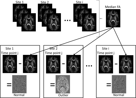
Schematic of the first step of the analysis framework: outlier identification. A median map is calculated for the desired tensor‐derived metric (for example, FA). Each individual time point FA image is subtracted from the median to identify outlier datasets.
The second analysis step is for the assessment of overall variance. Similar to the definition of the traditional ANOVA, one can compute the intrasite (i.e., within site) and the intersite (i.e., between sites) variances, on a voxel‐wise basis, creating maps of variance. Intrasite variance is computed by first calculating the variance across all time‐points for each site, then calculating the mean of the individual site variances. Intersite variance can be computed by first calculating the mean across all time‐points for each site, and then calculating the variance of the individual site means, as previously implemented by Zhu et al. for multicenter DTI variance analysis [Zhu et al., 2011]. In other words, we calculate the variance of the means and the mean of the variances; under the condition of no site bias, these two quantities should be equal. Sites are denoted as i = 1, 2, …, n and time points per site as j = 1, 2, …, m, and x ij is the image from site i at time point j, we then define the following quantities:
| (1) |
| (2) |
| (3a) |
| (3b) |
| (4a) |
| (4b) |
We define the intra‐ and intersite variability as the square root of their respective variances [Eqs. (3a) and (3b)], as in the relationship between variance and standard deviation. In addition, we define the intraclass and interclass correlation (ICC) coefficients [Kistner and Muller, 2004], which provide the fraction of variance attributed to intra‐ and intersite variance, respectively.
| (4) |
| (5) |
Data
The PedsMRI project had two “objectives”; Objective 1 enrolled a cohort of children over 5 years of age [Evans, 2006] and Objective 2 enrolled a younger cohort, between birth and 5 years of age [Almli et al., 2007]. The DTI protocol for Objectives 1 and 2 are identical with the exception of additional intermediate b value (b = 500 s mm−2) images for Objective 2. The majority of the phantom data was acquired under the Objective 1 protocol, and as such where the Objective 2 protocol was used the b = 500 s mm−2 data were removed, leaving identical protocols for all included data. The objective 1 DTI acquisition protocol specified a spin echo EPI sequence with minimum TR = 3 s, minimum achievable TE with full echo acquisition, axial slices (i.e., perpendicular to the z axis of the magnet, not oblique), field of view (FOV), matrix, and slice thickness adjusted to give 3 × 3 × 3 mm3 voxels, with the FOV and matrix size adjusted depending on the head size of the child. About 48–60 contiguous slices (no slice gaps), b values of 0 s mm−2 and 1,000 s mm−2 with six diffusion sensitization directions, repeated four times without averaging for a total of 28 brain volumes [4 × (1 × b = 0 s mm−2 + 6 × b = 1,000 s mm−2)]. Images were to be reconstructed at their native resolution, without zero filling or interpolation. No cardiac gating was applied. DTI data was acquired at five of the six participating PedsMRI centers (sites numbered 1 through 5, as defined in the public database at http://www.NIH-PediatricMRI.org), on a 1.5T magnet from either a Siemens scanner (three sites) or a GE scanner (two sites). Adherence to protocol was not 100%, and as such, there is some variability in these parameters across the living phantom and physical phantom scans, which are documented in Tables 1 and 2. T2 weighted (T2W) images were also acquired at each time point with a 2D PDW/T2W acquisition with TR = 3,500, TE1 = 17 ms, TE2 = 119 ms, axial slices, parallel to the anterior commissure‐posterior commissure (AC‐PC) plane, FOV = 250 × 220 mm2, matrix = 256 × 224, 80–90 slices of 2 mm thickness, as needed to cover the apex of the head to the bottom of the cerebellum. Each T2W scan for the living phantom was aligned to MNI space as described in the PedsMRI Objective 1 paper [Evans, 2006]. T2W scans for the physical phantom were aligned according to the ACR phantom specifications [ACR, 1998].
Table 1.
Description of living phantom datasets
| Site | Manufacturer | Time relative to first scan (days) | Brain coverage | Resolution (acquired) | Upsampling at scanner | Resolution (reconstructed) | slice thickness (mm) | Orientation of acquisition |
|---|---|---|---|---|---|---|---|---|
| 1** | Siemens | 26 | full | 3.0 | — | 3.0 | 3.0 | oblique |
| 1+ | Siemens | 297 | full | 3.0 | — | 3.0 | 3.0 | oblique |
| 1+ | Siemens | 626 | full | 3.0 | — | 3.0 | 3.0 | oblique |
| 1+ | Siemens | 1,059 | full | 3.0 | — | 3.0 | 3.0 | oblique |
| 2 | GE | 0 | cut—S,I | 3.0 | 128→256 | 1.48 | 3.0 | axial |
| 2 | GE | 273 | full | 3.0 | 128→256 | 1.48 | 3.0 | axial |
| 2+ | GE | 356 | full | 2.97 | — | 2.97 | 3.0 | axial |
| 2+ | GE | 1,218 | full | 2.97 | — | 2.97 | 3.0 | axial |
| 3+ | Siemens | 315 | full | 3.0 | — | 3.0 | 3.0 | axial |
| 3+ | Siemens | 978 | full | 3.0 | — | 3.0 | 3.0 | axial |
| 3+ | Siemens | 979 | full | 3.0 | — | 3.0 | 3.0 | axial |
| 4 | GE | 21 | cut—I | 3.13 | — | 3.13 | 4.0 | axial |
| 4+ | GE | 320 | cut—I | 3.13 | — | 3.13 | 4.0 | axial |
| 4+ | GE | 439 | full | 3.13 | 64→256 | 0.78 | 3.0 | axial |
| 4+ | GE | 553 | full | 2.81 | 128→256 | 1.41 | 3.0 | axial |
| 4+ | GE | 588 | full | 2.97 | — | 2.97 | 3.0 | axial |
| 4+ | GE | 588 | full | 2.97 | 64→256 | 0.74 | 3.0 | axial |
| 5+ | Siemens | 270 | full | 3.0 | — | 3.0 | 3.0 | oblique |
| 5+ | Siemens | 355 | full | 3.0 | — | 3.0 | 3.0 | oblique |
| 5 | Siemens | 444 | full | 3.0 | — | 3.0 | 3.0 | oblique |
| 5+ | Siemens | 940 | full | 3.0 | — | 3.0 | 3.0 | oblique |
| 5** | Siemens | 941 | full | 3.0 | — | 3.0 | 3.0 | oblique |
** = rejected, + = included in simulated data, S = superior, I = inferior.
Table 2.
Description of ACR phantom datasets
| Site | Time points | DWI repeats | Coverage | Resolution (acquired) | Upsampling at scanner | Resolution (reconstructed) | slice thickness (mm) |
|---|---|---|---|---|---|---|---|
| 1 | 1 | 4 | full | 4.0 | — | 4.0 | 3.0 |
| 27 | 1 | partial | 3.0 | — | 3.0 | 3.0 | |
| 6 | 1 | full | 3.0 | — | 3.0 | 3.0 | |
| 1 | 4 | full | 3.0 | — | 3.0 | 3.0 | |
| 2 | 2 | 1 | full | 2.97 | 64→256 | 0.74 | 3.0 |
| 1 | 2 | full | 2.97 | 64→256 | 0.74 | 3.0 | |
| 3 | 4 | full | 2.97 | 128→256 | 1.48 | 3.0 | |
| 1 | 5 | full | 2.97 | 128→256 | 1.48 | 3.0 | |
| 3 | 1 | full | 2.97 | — | 2.97 | 3.0 | |
| 1 | 3 | full | 2.97 | — | 2.97 | 3.0 | |
| 17 | 4 | full | 2.97 | — | 2.97 | 3.0 | |
| 3 | 1 | 4 | full | 3.44 | — | 3.44 | 3.0 |
| 1 | 4 | full | 3.36 | — | 3.36 | 3.0 | |
| 1 | 4 | full | 3.30 | — | 3.30 | 3.0 | |
| 1 | 4 | full | 3.22 | — | 3.22 | 3.0 | |
| 2 | 4 | full | 3.06 | — | 3.06 | 3.0 | |
| 38 | 1 | full | 3.0 | — | 3.0 | 3.0 | |
| 2 | 2 | full | 3.0 | — | 3.0 | 3.0 | |
| 2 | 3 | full | 3.0 | — | 3.0 | 3.0 | |
| 31 | 4 | full | 3.0 | — | 3.0 | 3.0 | |
| 4 | 1 | 2 | full | 3.13 | — | 3.13 | 4.0 |
| 1 | 3 | full | 3.13 | — | 3.13 | 4.0 | |
| 1 | 4 | full | 3.13 | — | 3.13 | 4.0 | |
| 1 | 2 | full | 2.81 | 128→256 | 1.41 | 3.0 | |
| 2 | 2 | full | 2.97 | 128→256 | 1.48 | 3.0 | |
| 3 | 4 | full | 2.97 | 128→256 | 1.48 | 3.0 | |
| 1 | 1 | full | 2.97 | — | 2.97 | 3.0 | |
| 2 | 2 | full | 2.97 | — | 2.97 | 3.0 | |
| 1 | 3 | full | 2.97 | — | 2.97 | 3.0 | |
| 1 | 4 | full | 2.97 | — | 2.97 | 3.0 | |
| 5 | 1 | 2 | full | 3.0 | — | 3.0 | 3.0 |
| 21 | 4 | full | 3.0 | — | 3.0 | 3.0 |
Total scans = 178, Total scans according to protocol = 71.
For this work, all T2W images were rigidly coregistered using FLIRT from the FSL package [Jenkinson et al., 2002] to one time point which was determined to be the highest quality scan by visual inspection, independently determined for the physical phantom and the living phantom. DTI data was processed with the TORTOISE processing pipeline [Pierpaoli et al., 2010], mainly: (1) Eddy current distortion and motion correction [Rohde et al., 2004], (2) susceptibility‐induced EPI distortion correction [Wu et al., 2008], using the T2W image as a target for registration, (3) rigid reorientation into a common final space defined by the registered T2W image. All corrections were performed in the native space of the diffusion weighted images (DWIs), all transformations were applied in a single interpolation step, and the b‐matrix was reoriented appropriately [Rohde et al., 2004].
Validation With Simulated Data
Using only the highest quality time points from the living phantom data (N = 16), we performed a tensor‐based registration using a nonparametric, diffeomorphic deformable image registration technique implemented in DTI‐TK [Zhang et al., 2007], that incrementally estimates its displacement field using a tensor‐based registration formulation [Zhang et al., 2005], to create a mean living phantom tensor. We then used this mean tensor to create synthetic DWIs with a known Gaussian distribution of noise, as previously described [Chang et al., 2007]. This was repeated 100 times, to simulate fictional multicenter studies with varying numbers of sites and scans per site. The noise value used, 12.5, is the mean signal standard deviation (SD) measured from the residuals of the tensor fit [Walker et al., 2011] from the individual living phantom scans, which results in an SNR of the b0 images of ∼ 40. Additional datasets were simulated to have lower SNR, using signal SD at two times baseline = 25.0 (SNR ∼ 15) and 10 times baseline = 125.0 (SNR ∼ 5). Nonlinear tensor fitting was performed on all simulated DWI datasets to generate synthetic tensors, and subsequently compute FA and Trace(D) maps. In addition, we added 10%, and subtracted 10% from FA and Trace(D) images (12.5 signal standard deviation) to create synthetic maps with a bias.
Five scenarios which are representative of real data situations were tested. In these scenarios, sites had a combination of “good” data, tensor‐derived metric maps from low SNR DWIs and/or biased tensor‐derived metric maps. Biased metric maps could be considered occasional outliers, while data computed from low SNR DWIs are representative of different intrinsic noise levels. Both could be indicative of site‐specific systematic differences. The five scenarios are
The ideal case—only good data at all sites
Minor outliers—10% outlier datasets introduced
Minor noise differences—10% low SNR datasets introduced
Systematic site bias—one site contains all biased images
Systematic noise difference—one site contains all noisy DWI datasets
All scenarios were tested with a balanced number of scans per site (10 sites, 10 scans per site). In addition, Scenarios 1–3 were also tested with an unbalanced number of scans per site, according to the distribution of living phantom datasets, i.e., five sites with N = [3,4,3,6,4], respectively (see Living Phantom section below).
Application to Phantom Data From the PedsMRI
Physical phantom
The physical phantom used by the PedsMRI project is the ACR MRI accreditation phantom [ACR, 1998]. It is a cylindrical phantom constructed of acrylate plastic, glass, and silicone rubber. The phantom is filled with 10 millimolar (mmol) nickel chloride solution containing sodium chloride (45 mmol) to simulate biological conductivity. The contrast vial contains 20 mmol nickel chloride and 15 mmol sodium chloride solution. The phantom contains a number of structures designed to measure the amount and type of distortion in structural T1‐ and T2‐weighted scans.
A total of 202 DTI scans were acquired at the five sites, with 24 scans rejected because of large deviations from the acquisition protocol or severe artifacts for a total of 178 successful DTI scans (Table 2). Of these 178 successful scans, 71 were acquired strictly according to protocol. Sites 1 and 4 each only acquired one scan according to protocol, and as such we were not able to perform any voxel‐wise variance analysis of these two sites. Thus, the framework is applied to a total of only 69 scans from Sites 2, 3, and 5 for the physical phantom. These 69 scans are unequally distributed across sites, so the framework was applied both to the full 69 datasets, as well as to a balanced set with 17 scans per site.
Living phantom
The living phantom is a healthy adult male aged 51 years at first scan. A total of 22 DTI scans were acquired at the five sites over 5 years (Table 1). It is assumed that the living phantom brain is stable over this time and any aging related variability is much smaller than inter‐ and intrasite variability. The datasets were assessed for gross artifacts before the analysis framework was applied. One time point was rejected due to severe ghosting, and one time point was rejected due to extremely low SNR. 20 datasets remained that were acceptable for voxel‐wise analysis. While these 20 scans are not equally distributed across the sites, the number of scans is small and as such a balanced dataset was not assessed.
Additionally, data were output from TORTOISE both with and without the EPI distortion correction applied. The framework was applied in both situations to assess the impact of preprocessing of DTI data on variance.
The results of the analysis framework for both the ACR and living phantom data are used to make inferences about the quality of the multicenter data, including whether there are site and/or time‐specific biases or increased variance due to systematic site effects.
RESULTS
Validation With Simulated Data
Outlier identification analysis successfully identified all simulated datasets with an introduced bias and low SNR. Representative images from each of the five scenarios are shown in Figure 2. In the ideal case, where no bias or difference in SNR exists between sites and scans (Test 1), then the difference from median is essentially zero; the maps show a slightly noisy distribution with no particular pattern or structure. With an introduced positive or negative bias of 10%, the intensity of FA and Trace(D) are increased or decreased, respectively, and show a structure that mimics the features of the FA and Trace(D) images, respectively. With low SNR, both at 2 and 10 times the baseline SD, FA is increased and Trace(D) is decreased in comparison to median. This is expected due to the previously described behavior of tensor‐derived metrics; as SNR decreases, FA becomes more positively biased [Pierpaoli and Basser, 1996], while Trace(D) becomes more negatively biased [Jones and Basser, 2004; Pierpaoli and Basser, 1996]. When a site is systematically different from the other sites, either with a bias or low SNR, it results in a shift of the median value toward the biased images, resulting in a slightly nonzero difference from median for nonaffected images of the simulation. This is most clearly visible by comparing Trace(D) in Tests 4 and 5 (Fig. 2), where the first five (unaffected) images shown are negative when a positive bias is introduced and positive when low SNR images are introduced. If one compares these unaffected images with all images from Test 1, one can see a small difference in intensity despite these images having the same intrinsic SNR.
Figure 2.
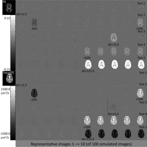
Sample difference from median maps for the simulated data validation tests for outlier identification. Bias and noise levels are indicated below the affected images. The outlier identification step clearly identifies data sets with both a bias and low SNR.
Intersite and intrasite variance in the ideal case, where no differences in SNR or biases exist, should be of the same magnitude indicating that no site bias exists and that the amount of variance is comparable within each site and across sites; this is the basis of the ANOVA F test under a null hypothesis of no site effects. Thus, the ICC values in the ideal case (Test 1) should be ICCinter = ICCintra = 0.5. Deviations from this would indicate whether the data has greater intersite variance or greater intrasite variance. On the basis of our classical definitions of intersite and intrasite variance, we would expect to find greater ICCinter in cases where the mean value differs between sites, while greater ICCintra would be found in cases where the within‐site variance differs between sites.
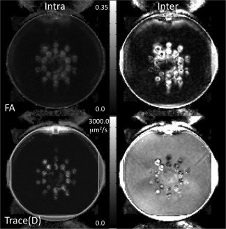
Figure 3 shows the intersite and intrasite variability maps for Test 1 for FA and Trace(D). Test 1 is an ideal case, and as such we expect these maps to be of the same magnitude. While the intersite variability map tends to have a noisier appearance than the intrasite variability map, their intensity is of similar magnitude. Both inter‐ and intrasite variability maps show greater variability in more anisotropic regions. Figure 4 shows the ICC maps for the five simulated test scenarios, and Table 3 gives the mean ICC values for the slice shown in Figure 4. As expected, the ideal scenario (Test 1) has ICCinter and ICCintra near 0.5, although the contribution of intersite variability tends to be slightly lower than the intrasite contribution. A similar result is seen for the cases of minor occurrences of bias (Test 2). Inclusion of low SNR datasets resulted in increased ICCintra, although only slightly different than the ideal case. When a single site is systematically different either with a bias or low SNR, the intersite variability is overall much greater than the intrasite variability. For FA, the effects are dependent on the level of anisotropy. When a site is biased, intersite variability is greatest at higher anisotropy. When a site contains noisy images, the intrasite variability becomes greater at higher anisotropy.
Figure 3.
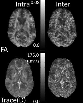
Intersite and intrasite variability maps of FA and Trace(D) for simulated data.
Figure 4.
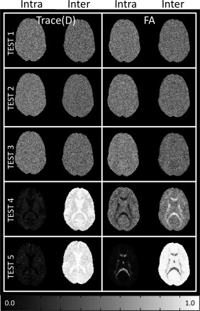
ICC maps for simulated data. No site difference is indicated when inter and intrasite ICC are equal (ICCinter = ICCintra = 0.5).
Table 3.
ICC values for simulated data (ICCinter = ICCintra = 0.5 indicates no site effect)
| FA | Trace (D) | |||
|---|---|---|---|---|
| ICCinter | ICCintra | ICCinter | ICCintra | |
| Test no. | Balanced number of scans | |||
| 1 | 0.48 | 0.52 | 0.47 | 0.52 |
| 2 | 0.48 | 0.52 | 0.46 | 0.53 |
| 3 | 0.45 | 0.54 | 0.48 | 0.52 |
| 4 | 0.56 | 0.44 | 0.91 | 0.08 |
| 5 | 0.93 | 0.06 | 0.93 | 0.07 |
| Test no. | Unbalanced number of scans | |||
| 1 | 0.46 | 0.53 | 0.47 | 0.53 |
| 2 | 0.46 | 0.53 | 0.53 | 0.47 |
| 3 | 0.43 | 0.57 | 0.47 | 0.53 |
When using an unbalanced number of scans, the results were similar to the balanced case. Outlier detection successfully identified all datasets with either a bias or low SNR. Intersite and intrasite variance was similar between the balanced and unbalanced cases. For the ideal case, the result was identical, with values close to 0.5, but slightly higher ICCintra. For Tests 2 and 3, we introduced ∼ 20% biased or low SNR datasets. In these cases, the ICC values are still close to 0.5, however, with biased images, the ICCinter is higher than ICCintra for Trace(D).
Application to Phantom Data From the PedsMRI
Physical phantom
For the ACR phantom data, we tested all 69 scans from three sites, as well as a balanced set with 17 scans per site (N = 51). Figure 5 shows a few representative difference from median images of Trace(D) for the ACR phantom scans. The first two time points of Site 2 have elevated Trace(D) compared to the median. Site 3 has no identifiable outliers, but has uniformly elevated Trace(D) compared to the median in all time points. Site 5 has two time points with greatly reduced Trace(D) (one shown in Fig. 5), and one time point with slightly reduced Trace(D) (not pictured). The FA maps for the ACR phantom (not pictured) should ideally be close to zero, but in reality have a complex anisotropic structure, particularly at the interfaces of the internal structures of the ACR phantom, making interpretation of FA data from the ACR difficult. All time points from Site 3 show a very slightly reduced FA compared to median, and the Site 5 time point with slightly reduce Trace(D) has an associated elevated FA with a heterogeneous appearance.
Figure 5.
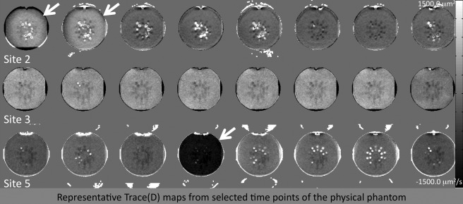
Difference from median maps for the PedsMRI physical phantom. Site 3 clearly shows a significant site difference compared to Sites 2 and 5.
Intersite variability is much greater than intrasite variability for Trace(D) and slightly greater for FA (Fig. 6), which is reflected in the much greater contribution of ICCinter (Table 4). This finding logically follows from the results of the outlier detection tool (Fig. 5) which showed a major site effect from Site 3, with a consistently higher value of Trace(D) compared to median for the study. The same results are seen both in the balanced and unbalanced tests. Because of the magnitude of the site effect, the variability maps are shown as they proved more informative than the ICC maps.
Figure 6.
Inter‐ and intrasite variability maps for the PedsMRI physical phantom. Intersite variability is clearly greater than intrasite variability, indicating a significant site difference.
Table 4.
ICC values for ACR phantom
| FA | Trace (D) | |||
|---|---|---|---|---|
| ICCinter | ICCintra | ICCinter | ICCintra | |
| Balanced case, N = 51 | 0.67 | 0.33 | 0.92 | 0.08 |
| Unbalanced case, N = 69 | 0.72 | 0.28 | 0.94 | 0.06 |
Living phantom
With the living phantom data, the outlier identification tool revealed two outliers from Site 2 with large deviation from median, showing reduced FA and elevated Trace(D), indicated by the black hashed circles in Figure 7. These outliers closely resemble the biased images from the simulated tests, with a structured pattern. In addition, two datasets from Site 4 also show reduced FA and elevated Trace(D), indicated by white circles. In these two datasets, the images appear more like the simulated datasets with different SNR with a more homogeneous appearance. Finally, one dataset from Site 5 shows elevated FA, but relatively normal Trace(D).
Figure 7.
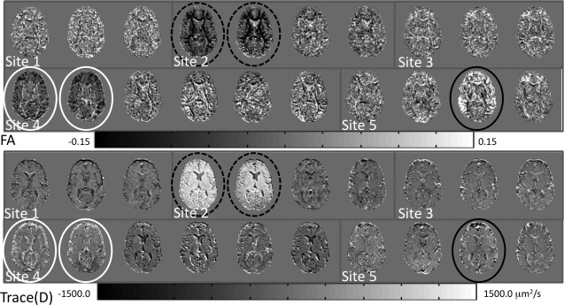
Difference from median maps for the PedsMRI living phantom data. Datasets identified as outliers are marked by white, solid and hashed black circles.
In the living phantom data, we also tested whether intersite and intrasite variability is affected by the type of image distortion correction scheme that is used. Thus, intersite and intrasite variability was calculated with and without the use of EPI distortion correction. This was done because EPI distortion correction is often neglected in DTI preprocessing pipelines, but recent work has shown it to be an important component of a DTI preprocessing pipeline [Andersson et al., 2003; Embleton et al., 2010; Irfanoglu et al., 2010; Wu et al., 2008]. Figure 8 shows the intersite and intrasite variability maps of FA and Trace(D). Again, the variability maps provided more anatomical information than the ICC maps, and as such were selected for visualization. On average, in the parenchyma, intersite variability is elevated compared to intrasite variability for both FA and Trace(D). This effect is amplified at tissue interfaces within the brain, suggesting inconsistent morphology and/or misregistration of the living phantom time points, potentially caused by a systematic site difference. In particular, large intersite variability is seen in the frontal lobes and genu of the corpus callosum; brain regions previously shown to be affected by susceptibility‐induced EPI distortions [Wu et al., 2008]. Variance analysis after EPI correction shows that this regionally increased intersite variability is dramatically reduced, although not completely eliminated. Because of the heterogeneous nature of the variability seen in the living phantom data, ICC values were collected in 4 ROIs (Table 5): two regions with average levels of intersite variability (temporal containing a mix of gray matter and white matter, and occipital white matter) and two regions with strongly elevated intersite variability (genu of the corpus callosum and frontal containing a mix of gray matter and white matter). All regions show greater ICCinter than ICCintra, both before and after EPI correction. However, the frontal region and genu of the corpus callosum show significant reduction in ICCinter after correction.
Figure 8.
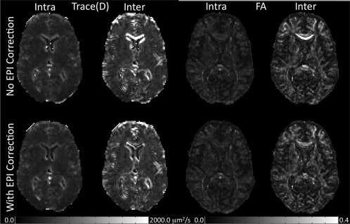
Inter‐ and intrasite variability maps for the PedsMRI living phantom data. Intersite variability is greater than intrasite variability. This is strongest at csf/tissue and white matter/gray matter interfaces, indicating significant misregistration between sites.
Table 5.
ICC values for living phantom
| Region | FA | Trace(D) | ||
|---|---|---|---|---|
| ICCinter | ICCintra | ICCinter | ICCintra | |
| Without EPI correction | ||||
| Temporal (GM) | 0.52 | 0.48 | 0.60 | 0.40 |
| Genu (WM) | 0.97 | 0.03 | 0.84 | 0.16 |
| Frontal (GM/WM) | 0.73 | 0.27 | 0.72 | 0.16 |
| Occipital (WM) | 0.65 | 0.35 | 0.61 | 0.39 |
| With EPI correction | ||||
| Temporal (GM) | 0.51 | 0.49 | 0.60 | 0.40 |
| Genu (WM) | 0.79 | 0.21 | 0.78 | 0.22 |
| Frontal (GM/WM) | 0.70 | 0.30 | 0.65 | 0.35 |
| Occipital (WM) | 0.64 | 0.36 | 0.60 | 0.40 |
| With EPI correction and outliers removed | ||||
| Temporal (GM) | 0.51 | 0.49 | 0.72 | 0.28 |
| Genu (WM) | 0.77 | 0.23 | 0.71 | 0.29 |
| Frontal (GM/WM) | 0.65 | 0.35 | 0.64 | 0.36 |
| Occipital (WM) | 0.61 | 0.39 | 0.69 | 0.31 |
These results include all 20 living phantom datasets. However, the outlier identification step indicates that certain datasets should not be included in this type of parametric analysis of variance. Therefore, this analysis was repeated using 15 of the 20 living phantom scans, with EPI correction applied, with a distribution at the five sites of N = [3,2,3,4,3] respectively. After removal of the outliers, ICCinter decreased, and ICCintra increased, although they did not reach the ideal value of 0.5 each. For Trace(D), however, with the outliers removed, the ICCinter is greater than when all 20 subjects are included.
DISCUSSION
Use of phantoms in multicenter DTI studies is necessary for assessing potential issues with data quality and understanding the sources of variance in data that we wish to pool over multiple sites and scanners. In this work, we propose a two‐step analysis framework for multicenter DTI study analysis that can identify problematic outlier datasets and indicate if there is a significant site effect in the variance of the data. We presented validation of the tools using simulated data, as well as results from the PedsMRI multicenter study.
Outlier identification is based on calculating the distance of each dataset from the median calculated from all datasets. With the simulated data, the tool was able to identify all datasets with an introduced bias, as well as all datasets with low SNR. Because DTI‐derived metrics such as FA and Trace(D) are biased by noise, the outlier identification step is ideal for identifying datasets affected by both biased data and noisy data. This step is a qualitative assessment, as the median value of all data is influenced by the datasets themselves. For instance, in the tests where a single site was systematically different, both the biased/low SNR datasets and the unaffected time points differed from the median, with the “good” data shifted a very small amount in the opposite direction of the “bad” data. However, this tool is still useful as a diagnostic for outliers, as it indicates that one set of data differs substantially from the median, while the remaining data differs only slightly. It is important to note that the median value is used instead of the mean value precisely for this reason. The mean value is strongly affected by outliers, while the median value is generally robust to outliers. In the case of a systematic difference, the presence of a large number of outlier data points results in only a small shift of the median value, allowing for a clear identification of problematic data points.
An incidental finding of the variance analysis in simulated brain data is higher variance of FA in white matter structures (Fig. 3). Using Monte Carlo simulations, Pierpaoli et al. [1996] showed that for constant SNR the variance of FA increases as anisotropy decreases, and that for a given anisotropy, the variance of FA increases as SNR decreases. The tensors in our simulations were derived from real human brain data where SNR is not constant—it is lower in white matter than in gray matter and CSF because of the strong T2* weighting of the DWIs. In our results, the observed larger variance in white matter regions is consistent with the presence of lower SNR in white matter. Interestingly, the effect of the reduction of SNR in white matter overcomes the variance reduction expected because of the higher anisotropy. Our results are in agreement with those of Chang et al. [2007], who presented similar maps of variance of FA from simulations of human brain data. However, our results are in apparent disagreement with the observations of several DTI investigations of data quality and reproducibility [Farrell et al., 2007; Heim et al., 2004; Marenco et al., 2006] that reported larger variability of FA in gray matter than in white matter. It should be noticed, however, that as a metric of FA variability these works did not use the variance of FA but its coefficient of variation (CoV). CoV is defined as the variance divided by the mean. We argue that in isotropic regions, CoV is not an appropriate metric for FA variability, because as the denominator of the fraction approaches zero, the values of CoV become very large and virtually meaningless. We believe that the use of CoV(FA) is at the basis of the very larger variability of FA found by these papers in gray matter regions.
Both the outlier identification and the variance analysis steps of the framework are targeted at identifying problems in multicenter data. We do not, however, offer specific solutions for the correction of these problems. When outliers occur in real data, further investigation is needed to reveal the cause of the issue. Only once the cause of the problem is identified might it be possible to construct a solution. In some instances, it may not be possible to correct all encountered problems. A prime example of this can be seen from the ACR and living phantom data of the PedsMRI. Site 2 shows two ACR time points with elevated Trace(D) and apparently normal FA, and two living phantom time points with elevated Trace(D) and low FA. These four time points occur only at the beginning of the study. Shortly after the latest of these four time points, the scanner at Site 2 underwent a software upgrade, after which FA and Trace(D) values appear to return to normal. The particular combination of elevated Trace(D) and depressed FA suggested that these data were acquired with a higher maximum b value than was assumed in fitting the tensor. Further investigation suggested that a maximum b value of ∼ 1,500 s mm−2 rather than 1,000 s mm−2 would be required to achieve the values of Trace(D) seen in these time points. As a potential solution, we adjusted the b matrix accordingly and were able to correct the measures of diffusivity such as Trace(D). However, the low anisotropy values cannot be corrected in this way. This is because the shape of the diffusion displacement profile becomes distorted at higher b values; the measured signal attenuates to the point that it reaches the level of the noise, resulting in an inability to properly estimate the eigenvalues and an artificially decreased value of anisotropy [Jones and Basser, 2004; Koay et al., 2009]. This difference in measured anisotropy due to a change in acquisition means that these datasets cannot be included in a standardized database. By detecting these outliers in the phantom data, we were able to identify 45 similarly affected subject datasets from the same site and time period in the PedsMRI study and reject them from public release and any further analysis.
Additionally, three ACR time points from Site 5 were identified as outliers. Two of these had similar behavior, with a dramatic decrease in Trace(D) value, and a slight increase in FA value. Upon further inspection of these two datasets, it was determined that the DTI data was incomplete, missing 1 DWI volume, resulting in a total of 27 vol. instead of the prescribed 28 vol. The outlier Trace(D) and FA values are then attributed to an incorrect mapping of the gradient table to the DWIs. If the missing volume were documented by the site, it would be possible to create an amended gradient table with which to potentially correct these outlier data points. With respect to this issue, no similar datasets were seen in the PedsMRI project data.
The third ACR outlier dataset from Site 5 showed low Trace(D) and dramatically elevated FA. On further inspection, the SNR of the DWIs of this dataset was very low, resulting in a large bias in the anisotropy values. This appeared to be an isolated occurrence, as subject datasets from the time period were assessed for SNR issues, but none were found.
Two Living Phantom time points from Site 4 had low Trace(D) and elevated FA. Similar to Site 2, Site 4 underwent a software upgrade shortly after these two time points. In addition, these datasets were acquired with an incorrect slice thickness of 4 mm and had eddy current distortions that were of a severity not correctable by any correction algorithm available to us. Because of the simultaneous occurrence of these three problems, all of which were uncorrectable, similarly affected data in the project should be rejected. We identified 135 datasets from Site 4 with these issues and removed them before public release.
Finally, site 5 had one living phantom time point with elevated FA and relatively normal Trace(D). The pattern of increase in FA was particularly elevated along the right and left sides of the brain with a section in the middle less affected. Further investigation of this data showed ghosting in the DWIs with a heterogeneous intensity, modulating from left to right (Fig. 9). Thirteen similarly affected subject datasets from the PedsMRI project were identified and removed from public release.
Figure 9.
Example of a ghosting artifact that resulted in an outlier dataset from the PedsMRI living phantom data.
In addition to isolated outliers, Site 3 in the ACR phantom data showed a systematic increase in Trace(D) compared to the median, indicating a potential site effect which is clearly supported by the inter‐ and intrasite variability measures for the ACR phantom (Fig. 6). This pattern, however, is not found in the Living Phantom data, and there is no evidence of a systematic increase in Trace(D) values in the subject data from the PedsMRI. We believe that this highlights the fact that water phantoms such as the ACR phantom are not appropriate as a quantitative phantom for the assessment of DTI data. For instance, the diffusivity of water (or doped water as in the ACR phantom) is not close to the diffusivity of human brain tissue. The diffusivity is also quite sensitive to temperature, which was not carefully controlled or documented over time and from site to site in the PedsMRI project. Water, as a nonviscous fluid, is subject to convective flow, which creates pseudo‐anisotropy effects, resulting in modulated FA and Trace(D) values in seemingly isotropic regions. This effectively prevents assessment of hardware issues such as gradient nonlinearity. Additionally, the embedded structures of the ACR phantom that are designed for geometric calibration in structural MRI data create many edges and interfaces which results in susceptibility distortions and partial volume effects in DTI data, further corrupting the values of tensor‐derived metrics. Thus, it is difficult to pin‐point the cause of the systematic difference in Trace(D) and FA between Site 3 and the other sites. However, because the living phantom does not show similar behavior, it is reasonable to believe that this is an artifact of the phantom used and will not have an impact on the subject data of the PedsMRI. The use of a diffusion phantom, which has known diffusivity values close to human brain tissue such as those proposed by Tofts et al. [2000] and by Pierpaoli et al. [2009] is of utmost importance for a quantitative assessment of bias and variance. In addition, a compound with a viscosity high enough to have no anisotropy due to convective flow, and a known temperature profile, such as the one proposed by Pierpaoli et al. [2009], would be most appropriate as a phantom in multicenter studies using DTI data.
An additional observation of the outlier detection tool is that isolated outliers may not be identified in parametric variance testing. For instance, in the simulated data tests 2 and 3, where a moderate number of data points were corrupted, no strong difference is seen between the inter‐ and intrasite variability, indicating that there is no site effect. In fact, there truly is no site effect in these two tests, as the corrupted data points were spread equally throughout the different sites, allowing these problematic datasets to go undetected, highlighting the importance of the initial outlier identification step. Measures of intersite and intrasite variability were, however, able to detect systematic differences between sites, particularly as shown in Tests 4 and 5 (Fig. 4 and Table 3).
In the living phantom data, ICCinter is generally greater than ICCintra for both FA and Trace(D) in the parenchyma. This effect is amplified at the tissue interfaces, suggesting that inconsistent morphology is a significant issue. Interestingly, the contribution of misregistration to variability is less for intrasite variability than for the intersite variability (Fig. 8), indicating that registration of time points within each site is more accurate than across sites. In the PedsMRI both scanner manufacturers used an anterior–posterior phase encode direction, but one manufacturer used a positive blip, while the other used a negative blip. The consequence of this difference is that one results in a compressed tissue artifact, while the other results in a stretched tissue artifact, which produced significant morphological differences between sites. This type of susceptibility induced EPI distortion is correctable with EPI distortion correction techniques, and our results indicate that by using image registration‐based EPI distortion correction as implemented in TORTOISE, we are able to reduce the large regional variability. The ICC values before and after correction indicate a trend toward more equal ICCinter and ICCintra; however, the EPI correction is clearly not able to fully correct for this distortion induced increased intersite variability.
Interestingly, when outlier datasets were removed before performing the variance analysis step, the FA ICC values were improved compared to the ICC values which included the outliers. However, Trace(D) ICC values were significantly worsened, with a large contribution of ICCinter. On careful inspection of Figure 7, the nonoutlier Trace(D) maps of Site 2 and 4 appear systematically lower than those of Sites 1, 3, and 5. Sites 2 and 4 used GE scanners, while Sites 1, 3, and 5 used Siemens scanners. This means that inclusion of outliers in the variance analysis resulted in a so‐called “masking effect” [Barnett and Lewis, 1985], where the presence of extreme outliers masked the presence of smaller, and in this case systematic, outliers. This also means that a bias exists between GE and Siemens scanners in the PedsMRI DTI dataset, which must be considered before pooling of data within this study, and may suggest that use of a single scanner manufacturer in multicenter studies is better than using multiple manufacturers.
Overall, we found that by both identifying outliers and assessing inter‐ and intrasite variability, we can have some confidence in determining the appropriateness of pooling data from multiple sites and scanners. In an ideal situation, we would also include tools for correcting for site differences in cases where data varies from site to site, as is apparent in the PedsMRI data. However, the appropriate ways in which to do this with DTI data remains an open question. For instance, a number of works suggest incorporating measures of variance as covariates in group statistical analysis to account for variance differences across sites [Friedman et al., 2008; Pagani et al., 2010], although they do not suggest an appropriate method for accurate estimation of the variance. The recent work by Zhu et al. provides a potential method for estimation of variance using the wild bootstrapping technique [Zhu et al., 2011], although it is unclear whether wild bootstrapping is an appropriate method for variance estimation in the presence of physiological noise artifacts such as are persistent in DTI data [Jones and Pierpaoli, 2005; Pierpaoli et al., 2003; Skare and Andersson, 2001; Walker et al., 2011]. In fact, it is extremely difficult to make an accurate and precise noise estimation in DTI data, as, to our knowledge, no models exist that can predict the occurrences and impact of physiological noise. Additionally and importantly, it is evident that scanner and site differences in variance can be due to systematic biases in the tensor‐derived metrics, not only differences in variance between sites. In fact, the level of bias is intrinsically linked to the amount of noise in the DTI data [Farrell et al., 2007; Pierpaoli et al., 1996]. One study suggested the use of a global scaling factor for adjusting FA values in a multicenter study [Vollmar et al., 2010]; however, without a gold standard, it is unclear how a meaningful quantitative scaling factor should be determined. The optimal situation in a multicenter study is prevention and not a cure; in other words, collect good quality data from the beginning and perform continuous quality assurance of data as it is acquired. We propose that the framework presented here can be used at regular intervals during data acquisition to identify problems as they manifest. For earliest diagnosis of problems, outlier analysis can begin as early as after acquisition of two time points, and variance analysis can being after acquisition of three time points. This approach is applicable not only to multicenter studies, but is also useful for identifying problems with on‐going single scanner studies as well.
CONCLUSION
In this work, we present a two‐step analysis framework for the assessment of phantom data in a multicenter study, along with validation using simulated data in tests that mimic real data situations. Careful characterization of the contributions to variance in a multicenter study is extremely important for accurate quantitative analysis of DTI data. However, more work is needed to determine the best method of meaningfully combining data acquired at different sites. From our work on the NIH MRI study of normal brain development, it is clear to us that the causes of outlier datasets, as well as systematic site differences within a single study, do not always have the same origin, and as such, cannot necessarily be treated with only one solution. Indeed, not all problems can be corrected. Our recommendation for multicenter studies is to perform a well controlled and well designed study from the outset by eliminating or restricting sources of expected added variance at the stage of data acquisition, to avoid many of the possible confounds that can occur. Because of the challenging nature of acquiring DTI data on unsedated children, the DTI component of the PedsMRI study was ancillary to the main objective, and as such suffered from a lack of rapid, highly structured quality control during data acquisition. On the basis of our experiences, we propose that the framework developed here should be applied early in a study, and at frequent, regular intervals throughout the course of data acquisition to allow investigators to quickly identify and solve problems as they occur, thus preventing substantial data rejection. In that vein, we present the following recommendations.
Recommendations for Multicenter DTI Studies
Phantoms, both physical and living, are better than population studies to detect small deviations between sites and over time because of the added confounds of biological and morphological diversity in a population.
Continued monitoring of acquired data over time, using tools such as those proposed in this work, is important.
Assess phantom data before and after any software and/or hardware upgrades during the course of the study.
Accurate quantification of diffusivity is desirable. This requires a phantom with reliable, repeatable measurements. A diffusion phantom should be used for this purpose.
Acquire approximately equal numbers of phantom scans per site to enable a meaningful parametric analysis of phantom data. Our results suggest that exactly equal may not be necessary, but large differences in the number of scans may complicate the interpretation of variance analyses.
Use EPI distortion correction to improve susceptibility induced EPI distortions, which are a significant contributor to intersite variability.
Use of a single scanner manufacturer and software version may help to reduce site‐specific differences.
Use the framework presented in this study to assess data as it is acquired to promptly identify and correct problems in your study.
ACKNOWLEDGMENTS
The authors have no conflicts of interest to declare. The views herein do not necessarily represent the official views of the National Institute of Child Health and Human Development, the National Institute on Drug Abuse, the National Institute of Mental Health, the National Institute of Neurological Disorders and Stroke, the NIH, the US Department of Health and Human Services, or any other agency of the US Government.
REFERENCES
- ACR (1998):Phantom Test Guidance for the ACR MRI Accreditation Program.Reston, VA:American College of Radiology. [Google Scholar]
- Almli CR, Rivkin MJ, McKinstry RC (2007): The NIH MRI study of normal brain development (Objective‐2): Newborns, infants, toddlers, and preschoolers. Neuroimage 35:308–325. [DOI] [PubMed] [Google Scholar]
- Andersson JL, Skare S, Ashburner J (2003): How to correct susceptibility distortions in spin‐echo echo‐planar images: Application to diffusion tensor imaging. Neuroimage 20:870–888. [DOI] [PubMed] [Google Scholar]
- Barnett V, Lewis T (1985):Outliers in Statistical Data.New York:Wiley. [Google Scholar]
- Basser PJ, Mattiello J, LeBihan D (1994): Estimation of the effective self‐diffusion tensor from the NMR spin echo. J Magn Reson B 103:247–254. [DOI] [PubMed] [Google Scholar]
- Beaulieu C (2002): The basis of anisotropic water diffusion in the nervous system—A technical review. NMR Biomed 15:435–455. [DOI] [PubMed] [Google Scholar]
- Brown GG, Mathalon DH, Stern H, Ford J, Mueller B, Greve DN, McCarthy G, Voyvodic J, Glover G, Diaz M, Yetter E, Ozyurt IB, Jorgensen KW, Wible CG, Turner JA, Thompson WK, Potkin SG (2011): Multisite reliability of cognitive BOLD data. Neuroimage 54:2163–2175. [DOI] [PMC free article] [PubMed] [Google Scholar]
- Chang LC, Koay CG, Pierpaoli C, Basser PJ (2007): Variance of estimated DTI‐derived parameters via first‐order perturbation methods. Magn Reson Med 57:141–149. [DOI] [PubMed] [Google Scholar]
- Embleton KV, Haroon HA, Morris DM, Ralph MA, Parker GJ (2010): Distortion correction for diffusion‐weighted MRI tractography and fMRI in the temporal lobes. Hum Brain Mapp 31:1570–1587. [DOI] [PMC free article] [PubMed] [Google Scholar]
- Evans AC (2006): The NIH MRI study of normal brain development. Neuroimage 30:184–202. [DOI] [PubMed] [Google Scholar]
- Farrell JA, Landman BA, Jones CK, Smith SA, Prince JL, van Zijl PC, Mori S (2007): Effects of signal‐to‐noise ratio on the accuracy and reproducibility of diffusion tensor imaging‐derived fractional anisotropy, mean diffusivity, and principal eigenvector measurements at 1.5 T. J Magn Reson Imaging 26:756–767. [DOI] [PMC free article] [PubMed] [Google Scholar]
- Focke NK, Helms G, Kaspar S, Diederich C, Toth V, Dechent P, Mohr A, Paulus W (2011): Multisite voxel‐based morphometry—Not quite there yet. Neuroimage 56:1164–1170. [DOI] [PubMed] [Google Scholar]
- Friedman L, Stern H, Brown GG, Mathalon DH, Turner J, Glover GH, Gollub RL, Lauriello J, Lim KO, Cannon T, Greve DN, Bockholt HJ, Belger A, Mueller B, Doty MJ, He J, Wells W, Smyth P, Pieper S, Kim S, Kubicki M, Vangel M, Potkin SG (2008): Test‐retest and between‐site reliability in a multicenter fMRI study. Hum Brain Mapp 29:958–972. [DOI] [PMC free article] [PubMed] [Google Scholar]
- Fu L, Fonov V, Pike B, Evans AC, Collins DL (2006): Automated analysis of multisite MRI phantom data for the NIHPD project. Med Image Comput Comput Assist Interv 9( Part 2):144–151. [DOI] [PubMed] [Google Scholar]
- Gouttard S, Styner M, Prastawa M, Piven J, Gerig G (2008): Assessment of reliability of multisite neuroimaging via traveling phantom study. Med Image Comput Comput Assist Interv 11( Part 2):263–270. [DOI] [PMC free article] [PubMed] [Google Scholar]
- Heim S, Hahn K, Samann PG, Fahrmeir L, Auer, DP (2004): Assessing DTI data quality using bootstrap analysis. Magn Reson Med 52:582–589. [DOI] [PubMed] [Google Scholar]
- Irfanoglu MO, Walker L, Pierpaoli C (2010):Effect of Susceptibility Distortion and Phase Encoding Direction on Tract Consistency in Diffusion Tensor Imaging.Stockholm, Sweden:ISMRM 18th annual meeting. [Google Scholar]
- Jenkinson M, Bannister P, Brady M, Smith S (2002): Improved optimization for the robust and accurate linear registration and motion correction of brain images. Neuroimage 17:825–841. [DOI] [PubMed] [Google Scholar]
- Jones DK, Basser PJ (2004): Squashing peanuts and smashing pumpkins: How noise distorts diffusion‐weighted MR data. Magn Reson Med 52:979–993. [DOI] [PubMed] [Google Scholar]
- Jones DK, Pierpaoli C (2005):Contribution of Cardiac Pulsation to Variability of Tractography Results.Miami Beach, Florida:ISMRM 13th annual meeting. [Google Scholar]
- Kistner E, Muller K (2004): Exact distributions of intraclass correlation and Cronbach's alpha with Gaussian data and general covariance. Psychometrika 69:459–474. [DOI] [PMC free article] [PubMed] [Google Scholar]
- Koay CG, Ozarslan E, Basser PJ (2009): A signal transformational framework for breaking the noise floor and its applications in MRI. J Magn Reson 197:108–119. [DOI] [PMC free article] [PubMed] [Google Scholar]
- Marenco S, Rawlings R, Rohde GK, Barnett AS, Honea RA, Pierpaoli C, Weinberger DR (2006): Regional distribution of measurement error in diffusion tensor imaging. Psychiatry Res 147:69–78. [DOI] [PMC free article] [PubMed] [Google Scholar]
- Pagani E, Hirsch JG, Pouwels PJ, Horsfield MA, Perego E, Gass A, Roosendaal SD, Barkhof F, Agosta F, Rovaris M, Caputo D, Giorgio A, Palace J, Marino S, De Stefano N, Ropele S, Fazekas F, Filippi M (2010): Intercenter differences in diffusion tensor MRI acquisition. J Magn Reson Imaging 31:1458–1468. [DOI] [PubMed] [Google Scholar]
- Pfefferbaum A, Adalsteinsson E, Sullivan EV (2003): Replicability of diffusion tensor imaging measurements of fractional anisotropy and trace in brain. J Magn Reson Imaging 18:427–433. [DOI] [PubMed] [Google Scholar]
- Pierpaoli C, Basser PJ (1996): Toward a quantitative assessment of diffusion anisotropy. Magn Reson Med 36:893–906. [DOI] [PubMed] [Google Scholar]
- Pierpaoli C, Jezzard P, Basser PJ, Barnett A, Di Chiro G (1996): Diffusion tensor MR imaging of the human brain. Radiology 201:637–648. [DOI] [PubMed] [Google Scholar]
- Pierpaoli C, Marenco S, Rohde GK, Jones DK, Barnett AS (2003):Analyzing the Contribution of Cardiac Pulsation to the Variability of Quantities Derived From the Diffusion Tensor.Toronto, Ontario, Canada: ISMRM 11th annual meeting, pp70. [Google Scholar]
- Pierpaoli C, Sarlls J, Nevo U, Basser PJ, Horkay F (2009):Polyvinylpyrrolidone (PVP) Water Solutions as Isotropic Phantoms for Diffusion MRI Studies.Honolulu, Hawaii:ISMRM 17th annual meeting, p1414. [Google Scholar]
- Pierpaoli C, Walker L, Irfanoglu MO, Barnett AS, Chang L‐C, Koay CG, Pajevic S, Rohde GK, Sarlls J, Wu M (2010):TORTOISE: An Integrated Software Package for Processing of Diffusion MRI Data.Stockholm, Sweden:ISMRM 18th annual meeting. [Google Scholar]
- Rohde GK, Barnett AS, Basser PJ, Marenco S, Pierpaoli C (2004): Comprehensive approach for correction of motion and distortion in diffusion‐weighted MRI. Magn Reson Med 51:103–114. [DOI] [PubMed] [Google Scholar]
- Skare S, Andersson JL (2001): On the effects of gating in diffusion imaging of the brain using single shot EPI. Magn Reson Imaging 19:1125–1128. [DOI] [PubMed] [Google Scholar]
- Tofts PS, Lloyd D, Clark CA, Barker GJ, Parker GJ, McConville P, Baldock C, Pope JM (2000): Test liquids for quantitative MRI measurements of self‐diffusion coefficient in vivo. Magn Reson Med 43:368–374. [DOI] [PubMed] [Google Scholar]
- Vollmar C, O'Muircheartaigh J, Barker GJ, Symms MR, Thompson P, Kumari V, Duncan JS, Richardson MP, Koepp MJ (2010): Identical, but not the same: Intrasite and intersite reproducibility of fractional anisotropy measures on two 3.0T scanners. Neuroimage 51:1384–1394. [DOI] [PMC free article] [PubMed] [Google Scholar]
- Walker L, Chang LC, Koay CG, Sharma N, Cohen L, Verma R, Pierpaoli C (2011): Effects of physiological noise in population analysis of diffusion tensor MRI data. Neuroimage 54:1168–1177. [DOI] [PMC free article] [PubMed] [Google Scholar]
- Wu M, Chang L‐C, Walker L, Lemaitre H, Barnett AS, Marenco S, Pierpaoli C (2008): Comparison of EPI distortion correction methods in diffusion tensor MRI using a novel framework. Med Image Comput Comput Assist Interv Int Conf Med Image Comput Comput Assist Interv 11( Part 2):321–329. [DOI] [PMC free article] [PubMed] [Google Scholar]
- Zhang H, Yushkevich PA, Gee JC (2005): Deformable registration of diffusion tensor MR images with explicit orientation optimization. Med Image Comput Comput Assist Interv 8( Part 1):172–179. [DOI] [PubMed] [Google Scholar]
- Zhang H, Avants BB, Yushkevich PA, Woo JH, Wang S, McCluskey LF, Elman LB, Melhem ER, Gee JC (2007): High‐dimensional spatial normalization of diffusion tensor images improves the detection of white matter differences: An example study using amyotrophic lateral sclerosis. IEEE Trans Med Imaging 26:1585–1597. [DOI] [PubMed] [Google Scholar]
- Zhu T, Hu R, Qiu X, Taylor M, Tso Y, Yiannoutsos C, Navia B, Mori S, Ekholm S, Schifitto G, Zhong J (2011): Quantification of accuracy and precision of multicenter DTI measurements: A diffusion phantom and human brain study. Neuroimage 56:1398–1411. [DOI] [PMC free article] [PubMed] [Google Scholar]