Automating tumor classification with pixel-by-pixel contrast-enhanced ultrasound perfusion kinetics

Abstract

Contrast-enhanced ultrasound (CEUS) enables highly specific time-resolved imaging of vasculature by intravenous injection of ∼2 μm gas filled microbubbles. To develop a quantitative automated diagnosis of breast tumors with CEUS, breast tumors were induced in rats by administration of N-ethyl-N-nitrosourea. A bolus injection of microbubbles was administered and CEUS videos of each tumor were acquired for at least 3 min. The time-intensity curve of each pixel within a region of interest (ROI) was analyzed to measure kinetic parameters associated with the wash-in, peak enhancement, and wash-out phases of microbubble bolus injections since it was expected that the aberrant vascularity of malignant tumors will result in faster and more diverse perfusion kinetics versus those of benign lesions. Parameters were classified using linear discriminant analysis to differentiate between benign and malignant tumors and improve diagnostic accuracy. Preliminary results with a small dataset (10 tumors, 19 videos) show 100% accuracy with fivefold cross-validation testing using as few as two choice variables for training and validation. Several of the parameters which provided the best differentiation between malignant and benign tumors employed comparative analysis of all the pixels in the ROI including enhancement coverage, fractional enhancement coverage times, and the standard deviation of the envelope curve difference normalized to the mean of the peak frame. Analysis of combinations of five variables demonstrated that pixel-by-pixel analysis produced the most robust information for tumor diagnostics and achieved 5 times greater separation of benign and malignant cases than ROI-based analysis.

INTRODUCTION

In the United States, cancer is one of the top leading causes of death, second only to heart disease. In 2011, 1.6 × 10⁶ new cancer cases will be diagnosed and 600 000 deaths will be attributed to cancer.¹ Early detection and accurate diagnosis of cancer increase chances for survival by allowing treatment of the disease before it metastasizes and becomes intractable.^{2, 3} Diagnostic accuracy is equally important to providing patients with optimal therapy and controlling the rising cost of health care. Biopsy is the most accurate method of diagnosing cancer, but this method is invasive and is not always a viable option depending on the location of the tumor.^{4, 5, 6}

Medical imaging offers several modalities with the ability to detect and diagnose tumors noninvasively, including magnetic resonance imaging, positron emission tomography, x ray computed tomography, and ultrasound (US). Ultrasound provides good spatial and temporal resolution, is nonionizing and most affordable, allowing US to be safely performed on patients as frequently as necessary.^{7, 8} Recent advances over the past decade with contrast-enhanced ultrasound (CEUS) have significantly improved ultrasound’s diagnostic potential for cancer by intravenously injecting ∼2 μm gas filled microbubbles which, due to their size, are limited to the intravascular space. When given intravenously, they enhance all vessels including capillaries. Although capillaries cannot be resolved, capillary filling with microbubbles causes enhancement of perfused tissues. These properties allow for highly specific time-resolved imaging of tumor vasculature and perfusion.^{9, 10, 11, 12} Since cancers exhibit accelerated metabolism, they promote the development of new blood vessels; different types of cancers will often possess characteristic patterns to their vasculature which allow identification of the tumor type with CEUS.^{13, 14, 15}

Previous reports have shown that analysis of time-intensity curves (TICs) can produce hemodynamic measurements such as the area under the curve (AUC) and time to peak (TTP) that have statistical significance between benign and malignant lesions of various types of tumors.^{16, 17, 18} Since the CEUS imaging signal is noisy due to many factors, including speckle noise, motion, and fluctuations in the concentration of microbubbles, CEUS TIC analysis is nearly always applied to the mean of the signal intensity within a region of interest (ROI) surrounding the tumor.^{19, 20} This ROI analysis benefits from reduced noise and well behaved TICs. However, because the signal intensity is averaged across the tumor, this type of analysis is incapable of detecting spatial heterogeneity across the tumor and is inherently restricted to measuring perfusion parameters of the tumor as a whole. This may limit the diagnostic potential of systems relying on ROI analysis since intratumoral heterogeneity is known to change with tumor progression.^{21, 22, 23}

Instead of ROI analysis, CEUS videos have also been analyzed on a pixel-by-pixel (P × P) basis where the enhancement behavior of each pixel was analyzed and the CEUS video was transformed into one or more parametric images. Although P × P processing is more susceptible to noise and motion artifacts, analysis of the TIC on a P × P basis allows measurement of localized perfusion kinetics. For example, Pollard et al. measured the time to 20% maximum replenishment using CEUS destruction-reperfusion techniques in a rat kidney model pre- and post-treatment to detect tumor response to drug therapy.²⁴ Ellegala et al. analyzed tumor blood velocity, blood volume, and blood flow in a rat glioma model by fitting their data to an exponential model and showed that tumor blood velocity was typically lower and fractional blood volume typically greater than surrounding tissue.²⁵ Pysz et al. employed the maximum intensity persistence (MIP) algorithm and found that MIP imaging plateau values correlated with ex vivo microvessel density analysis and MIP imaging could detect tumor response to antiangiogenic therapy as early as 48 h after dose administration in a mouse model.²⁶ Comparing the relative enhancement patterns of focal liver lesions to normal liver tissue, Rognin et al. were able to improve a clinician’s diagnostic accuracy to 97% sensitivity and 91% specificity.²⁷

In this study, CEUS time-intensity curves were analyzed on a pixel-by-pixel basis to measure many hemodynamic parameters associated with the wash-in, peak enhancement, and wash-out phases of the microbubble bolus injection to detect the aberrant functionality of tumor vasculature. Linear discriminant analysis (LDA) was employed to semiautomatically classify CEUS videos as benign or malignant on the basis of these P × P TIC measurements. As far as we know, this is the first report combining P × P TIC analysis with LDA to develop a diagnostic system. This report also employs the standard deviations of the hemodynamic parameters and correlated measurements to improve the separation of benign and malignant classifications; these advances were enabled by combining motion correction with novel software noise suppression techniques.

METHODS

ENU rat tumor model

Sprague-Dawley rats were intraperitoneally injected with either a high (180 mg/kg) or low (45.5 mg/kg) dose of N-ethyl-N-nitrosourea (ENU, Sigma-Aldrich, St. Louis, MO), a well known carcinogen that frequently generates tumors in mammary glands; the high dose more frequently generates malignant tumors, and the low dose generates a mix of benign and malignant tumors.^{28, 29, 30, 31, 32} This study included the assessment of three rats with one benign tumor each and seven rats with one malignant tumor each that occurred between 6 weeks and 9 months after treatment with ENU. The tumor cross sectional areas as measured under ultrasound were approximately 1.50 ± 0.87 cm² for benign tumors and 2.37 ± 2.28 cm² for malignant tumors (mean ± standard deviation) and the difference between benign and malignant tumor sizes were not statistically significant (P > 0.05). Tumors that arose external to the mammary glands were excluded from the study.

All animals were euthanized immediately following their final ultrasound scan. Tumor tissue was dissected and sectioned at an orientation corresponding to the plane of the ultrasound image. The tissue was fixed in 10% formalin solution and embedded in paraffin. Histological slides of 5 μm-thick tumor slices were prepared and stained with hematoxylin and eosin in a standard fashion. All histologic processing was carried out by the UCSD Histology Core in the Moores Cancer Center. Histopathologic examinations of the tumors were limited to a malignant or benign diagnosis and were conducted by a skilled observer blinded to the US findings or ENU dose. The criteria included nuclear size, invasion of surrounding tissue, appearance of breast tissue ducts, and cell size.

Ultrasound imaging

Animals were anesthetized using inhaled isoflurane gas. Animals were unrestrained except when specific positioning was required to image the tumor, in which case tape was used to fix the animal’s position. Ultrasound imaging was performed using a Philips iU22 equipped with a L12-5 probe (Philips Medical Systems, Bothel, WA). The tumor imagining plane was chosen such that breathing motion was within the plane of imaging rather than across plane to allow for motion correction. The largest cross section of the tumor avoiding large cysts or obvious necrotic areas was chosen. Images were optimized by adjusting the field of view and gain. Once optimized, the transducer was mechanically fixed in position and control settings were not changed. A contrast-specific imaging mode was employed that transmitted unique pulses that resulted in unique signals from microbubbles to allow the subtraction of tissue signals in real-time. Because contrast specific modes resulted in blank images, a dual display depicted two images of the identical slice, one processed in standard B-mode for tissue imaging, and one processed for microbubble image. Imaging was acquired at 7 MHz, 0.06 mechanical index (MI) for contrast and 0.02 MI for B-mode, 6 Hz frame rate, with typically a 38 dB dynamic range, and the focal zone positioned at the depth of the tumor. These parameters resulted in a resolution along the depth (axial) and across the plane (lateral) of 0.6 × 0.6 mm, and a slice thickness of 1.6 mm at the focal zone.³³ With the cine capture turned on, a single bolus injection of ultrasound contrast was administered through the tail vein followed with a 2 mL saline flush, and the recording continued for 3 min to observe the wash-in and wash-out kinetic through the tumor slice. The cine clips were stored as videos with the Microsoft Video 1 (CRAM) lossy compression codec.

Multiple videos were collected of most rats to increase the sample size to 19 videos: Tumor histology revealed the benign or malignant nature of the tumor: 5 videos of 3 benign tumors and 14 of 7 malignant tumors (Table TABLE I.). Contrast agents used included BR38 (0.1 mL of stock solution, ∼10⁷ microbubbles), BR55 (0.1 mL of 1:10 dilution, ∼10⁷ microbubbles), and SonoVue (0.1 mL of stock solution, ∼10⁷ microbubbles) all from Bracco (Bracco Imaging SpA, Milano, Italy), Definity (0.2 mL of 1:10 dilution, ∼10⁹ microbubbles) (Lantheus Medical Imaging, Billerica, MA), and Visistar (0.15 mL of stock solution, ∼10⁸ microbubbles) and Visistar VEGFR2 (0.15 mL of stock solution, ∼10⁸ microbubbles) (Targeson, La Jolla, CA). All animals that were multiply imaged received at least one untargeted contrast agent and one targeted contrast agent. Out of the 5 videos of benign tumors, 3 (60%) employed untargeted microbubbles and 2 (40%) employed targeted microbubbles, similarly, 8 (57.1%) and 6 (42.9%) of the 14 videos of malignant tumors employed untargeted and targeted contrast agents, respectively. Since the microbubble kinetics of untargeted and targeted microbubbles administered across benign and malignant cases were only observed for only 3 min, their use should not bias the classification results. In the worst case, the use of targeted and nontargeted microbubbles should add variance to the perfusion measurements, reducing classification performance. In fact, malignant tumors had a faster washout than benign tumors, which was the opposite of what would be expected when targeted microbubbles are given that should accumulate in malignant tumor. Therefore the use of targeted microbubbles likely dampened the wash-out difference that was observed. Repeat injections were administered at least 10 min after the previous injection to provide ample time for the previously injected microbubbles to be cleared from circulation.

TABLE I.

Animal ID, histology of the tumor, video ID, contrast agent used, and targeting of the contrast agents are listed.

Rat	Histology	Video	Agent	Target
1	Malignant	1	BR38	None
		2	BR55	VEGFR2
2	Malignant	3	BR38	None
		4	BR55	VEGFR2
3	Benign	5	BR38	None
		6	BR55	VEGFR2
4	Benign	7	BR38	None
		8	BR55	VEGFR2
5	Malignant	9	BR38	None
		10	BR55	VEGFR2
6	Malignant	11	BR38	None
		12	BR55	VEGFR2
		13	SonoVue	None
7	Benign	14	BR38	None
8	Malignant	15	BR38	None
		16	BR55	VEGFR2
9	Malignant	17	Definity	None
10	Malignant	18	Visistar	None
		19	Visistar VEGFR2	VEGFR2

Image analysis

Analysis of contrast-enhanced ultrasound videos was performed using custom software developed in MATLAB (Mathworks, Natick, MA). The variables employed to characterize the TIC are listed in Table TABLE II.. The time-intensity curves were analyzed following motion correction on a pixel-by-pixel basis to measure several hemodynamic parameters associated with the wash-in, peak enhancement, and wash-out phases of the microbubble bolus injection to detect the aberrant functionality of tumor vasculature. TIC analysis on a pixel-by-pixel basis allows measurement of the local perfusion kinetics, but it is more susceptible to noise, speckle, and motion inherent to CEUS compared to previous reports of CEUS TIC analysis which applied only to the spatial mean of the intensity within a ROI surrounding the tumor.^{19, 20} Previous P × P based reports handled the problem of noise by either discarding misbehaving pixels,³⁴ fitting their data to simple mathematical models,^{24, 25} or by employing variables that were relatively insensitive to fluctuations within the signal.²⁷ In this report, noise was handled by two key preprocessing steps: (1) optimal selection of the reference frame independently for each video for accurate motion correction and (2) using noise filters optimized for each parameter.

TABLE II.

This table lists the kinetic measurements employed to parameterize the TIC, their acronyms, and the signal processing step(s) for each variable, and the effect of pixel-by-pixel measurement on the mean of each measurement. Throughout this report, variable acronyms suffixed with “_m” or “_s” indicate the mean or standard deviation of the pixel-by-pixel measurements within the ROI, respectively.

Acronym	Full name	Processing	Pixel
PI	peak intensity	LPF	No
TTP	time to peak	LPF	No
AUC	area under the curve	LPF	No
AUCWO	area under the curve: wash-out	LPF	No
FWHM	full width at half maximum	LPF	No
PGWI	peak gradient: wash-in	LPF	No
PW	peak width	LPF	No
MTT	mean transit time	LPF	No
WOT80	wash out time to 80% of peak	LPF	No
WOT50	wash out time to 50% of peak	LPF	No
WOT20	wash out time to 20% of peak	LPF	No
DIWO15	drop of intensity: wash out to 15 seconds	LPF	No
ISD	standard deviation of intensity	UNP	Yes
ISDN	standard deviation of intensity normalized to peak intensity	UNP	Yes
AUOC	area under the original TIC curve	UNP	No
AUEC	area under the envelope curve	ENV	No
OEDN	envelope curve difference normalized to the mean of the peak frame	UNP & ENV	Yes
PGWONM	peak gradient: wash-out normalized to the mean of the peak frame	LPF	No
PSWINM	peak slope: wash-in normalized to the mean of the peak frame	LPF	No
OEDNM	envelope curve difference normalized to the mean of the peak frame	UNP & ENV	Yes
TOA	time of arrival	THR	No
FECT_10	fractional enhancement coverage time: 10%	THR	Yes
FECT_20	fractional enhancement coverage time: 20%	THR	Yes
FECT_50	fractional enhancement coverage time: 50%	THR	Yes
FECT_80	fractional enhancement coverage time: 80%	THR	Yes
FECT_90	fractional enhancement coverage time: 90%	THR	Yes
Coverage	coverage	THR	Yes

Image registration

To minimize the impact of breathing motion on pixel-based measurements, an affine image registration technique that maximizes mutual information was applied to correct lateral motion throughout each CEUS video.³⁵ Image registration was performed on B-mode images (tissue image), and the resulting transformation parameters were applied to the contrast-specific images (microbubble only image). Rather than registering all frames sequentially³⁶ or arbitrarily choosing a single reference frame³⁷ as in previous reports, a unique image registration system was employed. All frames were registered to a single reference frame that was chosen by sampling 100 frames throughout each video and finding the frame which presented the greatest sum of squared correlation with all other sample frames. This additional selection criterion had the benefit of choosing a minimally disrupted reference point relative to the remaining image frames.

Although pixel similarity based registration methods such as this are computationally expensive, they eliminate the requirement for manual placement of fiduciary markers by an observer or a priori extraction of anatomic features as with feature based registration methods. Additionally, it has been shown that image similarity based techniques perform at least as well as feature based registration methods.^{35, 38, 39} Table TABLE III. shows the total sum of squared differences of B-mode pixel intensities from frame to frame as a metric of motion pre- and post-motion correction. Although motion was minimal prior to image registration (due to anaesthetization and immobilization of the rat and imaging probe), motion was further reduced after image registration was applied as indicated by the reduced sum of squared difference (SSD) values. Figure 1 shows the integrated intensity of each pixel over all frames within video 2 (a) pre and (b) post image registration. With the integrated intensity algorithm, motion within the videos should cause features to blur in the direction of motion. Although video 2 had the greatest percent decrease in SSD scores after motion correction, the two integrated intensity images look nearly identical and features can be seen sharply in both images, indicating that the premotion corrected videos were fairly stable. Even though minor motion artifacts were still present after image registration, the small fluctuations in intensity were filtered out by the low-pass filtering technique described below.

TABLE III.

Total sum of squared differences (SSD) from frame to frame of B-mode intensities within the tumor region of interest pre- and post-image registration. Due to anaesthetization and immobilization of the rats and US probe, there was little motion within the video other than minor breathing motion. Image registration lowered the SSD values, indicating reduced motion.

Video	SSD pre ( × 108 a.u.2)	SSD post ( × 108 a.u.2)	Percent decrease
1	28.0	20.2	− 27.8%
2	22.6	14.0	− 38.2%
3	10.7	8.22	− 23.4%
4	7.77	6.85	− 11.8%
5	3.37	2.99	− 11.2%
6	2.81	2.51	− 10.5%
7	6.52	5.57	− 14.5%
8	6.80	5.43	− 20.1%
9	3.33	2.65	− 20.5%
10	6.01	5.17	− 14.0%
11	22.5	15.9	− 29.4%
12	13.4	10.2	− 23.6%
13	15.3	11.9	− 22.6%
14	8.09	5.85	− 27.7%
15	9.83	8.16	− 17.0%
16	17.8	15.1	− 15.2%
17	64.5	48.7	− 24.5%
18	31.2	21.9	− 29.7%
19	25.4	18.9	− 25.5%

Figure 1.

Integrated intensity of B-mode frames pre and post image registration. The intensity of each pixel was integrated over all frames within video 2 (a) pre and (b) post image registration. With the integrated intensity algorithm, motion within the videos should cause features to blur. Although video 2 had the greatest percent decrease in sum of squared difference scores after motion correction (Table TABLE III.), the two integrated intensity images looked nearly identical; features can be seen sharply in both images.

Time-intensity curve processing and analysis

The compressed video signal of each pixel passed through one of three possible preprocessing steps depending on the kinetic parameter ultimately being measured: unprocessed; low pass filtering; and envelope curve detection. In Fig. 2, the effects of these preprocessing steps are demonstrated with TICs from a single representative pixel of a typical benign and malignant video. (1) The unprocessed TIC was used for a few measurements to quantify the fluctuations in the signal, e.g., the standard deviation of intensity (ISD) of each pixel over time. (2) To reduce the impact of noise artifacts, the video signal of each pixel was filtered with a low pass filter designed with a cutoff frequency at 0.125 Hz to eliminate noise spikes while preserving the shape of the bolus injection curve. Low pass filtering was used in the majority of measurements to capture the characteristics of the TIC. (3) An alternative step to low pass filtering was the calculation of an envelope function which captures the local peaks in the data and was subsequently used in envelope-curve related metrics. Measurements acquired from the envelope curve or the unprocessed data were used to quantify the fluctuations in the TIC caused by changes in microbubble concentration in each pixel. The processing steps applied for each variable are shown in Table TABLE II..

Figure 2.

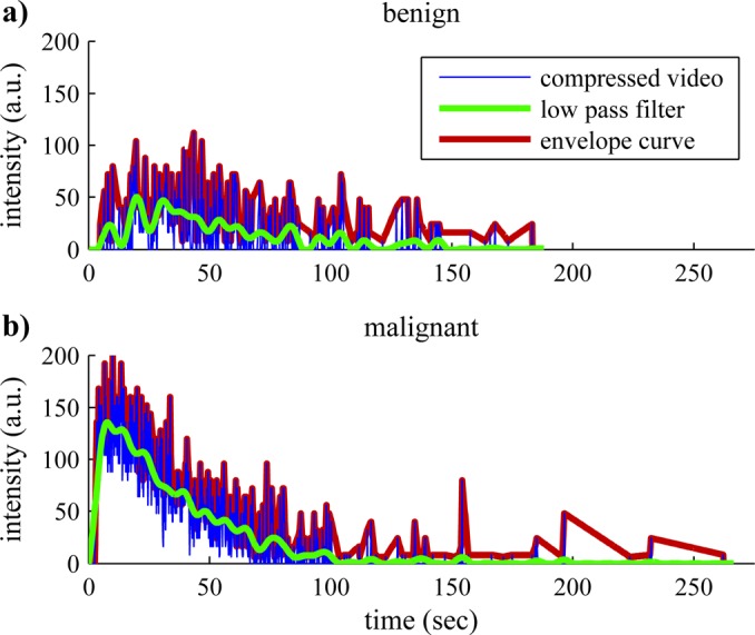
(Color online) Time-intensity curve preprocessing. Sample processing of the compressed video signal from a single representative pixel from a typical (a) benign and (b) malignant video. TICs for each pixel were either low pass filtered (LPF) or the envelope curve (EC) was detected prior to linearization. LPF allowed characterization of the overall wash-in and wash-out perfusion patterns, while EC and the unprocessed signal allowed detection of transient fluctuations in concentration of the contrast agent.

Following the above steps, the data were linearized to reverse the data compression employed by ultrasound imagers, producing a TIC linearly proportional to the ultrasound signal power and concentration of contrast agents.⁴⁰ Measurements of perfusion kinetics were mostly derived from these linearized TICs. In addition to the filters, to improve the robustness of the dataset against noise, multiple correlated variables were employed to make similar measurements. For example, multiple wash-out time (WOT) measurements were acquired which measure the time span between peak intensity to different percentages of peak intensity, e.g., 80% (WOT80), 50% (WOT50), and 20% (WOT20) of peak intensity. To quantify the overall tumor behavior as well as the tumor heterogeneity, the mean and standard deviation of each kinetic parameter was calculated within a ROI. The ROI was manually defined and tightly encompassed the enhanced perimeter of the tumor, but excluded any shadowed portion in the mid or far field. Necrotic regions of the tumor were included within the ROI, and all pixels within the ROI were used in TIC analysis.

A few of the basic kinetic differences between benign and malignant tumors in the ENU rat tumor model are readily observed in Fig. 2. Compared to the sample TIC from the benign tumor, the malignant tumor has a much higher peak intensity (PI) and reaches this peak intensity much more quickly. Since the intensity of the received ultrasound signal is proportional to the concentration of microbubbles within a pixel, and since microbubbles are limited to the intravascular space, a higher PI indicates greater fractional blood volume. Furthermore, the time it takes to reach peak intensity is inversely proportional to the blood flow velocity: faster blood flow velocity results in lower TTP measurements and vice versa. These observations were consistent with the expectation that malignant tumors are highly vascularized with large blood pools and high rates of blood flow. The noise in the single pixel data also helped discriminate between benign and malignant tumors including; for example, the standard deviation of the intensity normalized to the peak intensity of each pixel (ISDN)—a variable that measures the fluctuations of the intensity of each pixel over time. Abnormalities in malignant tumor vasculature such as shunts and variable sized capillaries lead to aberrant functionality and flow rates with greater spatial and temporal heterogeneity which were reflected in the ISDN measurements.

Image domain analysis

In addition to the quantitative measurements of the TIC, to capture parameters that mimic human eye observations, several measurements were derived from image threshold based techniques applied to the log-compressed video intensity signal. To determine a good threshold value for each video, the Otsu threshold method⁴¹ was applied to the first frame to achieve an integrated intensity at the midpoint between pre- and peak-enhancement under the assumption that this frame would contain a combination of enhanced and unenhanced pixels. Subsequently, this threshold value was applied to all frames to consistently segment the pixels with sufficient contrast enhancement from background. This enhancement information was applied to measure the time of arrival (TOA) of contrast agents, tumor enhancement coverage, and the various fractional enhancement coverage time (FECT) measurements. Similar to TIC analysis, the mean and standard deviation were used to summarize tumor TOA measurements, whereas coverage and FECT measurements already yield a single scalar value for the tumor ROI.

Classification

Classification optimization of cross-validation error

Linear discriminant analysis (LDA) was employed to classify the videos as either benign or malignant based on the kinetic measurements. As described above, means and standard deviations of the TIC measurements as well as threshold based measurements were used as input to the LDA classifier. All possible combinations of one or two variables were tested to determine the most predictive sets by performing a fivefold cross validation.

Classification optimization with the Fisher discriminant criterion

In order to further characterize performance of LDA classification with more than two variables, subsets composed of combinations of five variables were ranked based on the Fisher linear discriminant criterion function:

$$\mathrm{J}=\frac{{|{\mu }_{\mathrm{M}}-{\mu }_{\mathrm{B}}|}^2}{{\mathrm{S}}_{\mathrm{M}}^2-{\mathrm{S}}_{\mathrm{B}}^2},$$ (1)

where µ_M, µ_B, S_M, and S_B are the means and scatters of the LDA score for malignant and benign tumors, respectively. To investigate the relative importance of pixel kinetics, every combination of five variables were entered into the LDA classifier for training and ranking (>30 × 10⁶ combinations). Combinations were arbitrarily limited to five variables to limit the time requirement of processing. These combinations of variables were manually categorized into four groups: mean-based variables versus standard deviation-based variables; and nonpixel-by-pixel (non-P × P) variables versus P × P variables. The groups were designed to quantify the importance of the pixel-by-pixel kinetics because most of the mean-based measurements (for example, peak intensity (PI) and AUC) do not benefit from analyses of individual pixel TICs and can be mimicked by analyses that take the mean of the intensity within the ROI prior to analysis, similar to previously published reports. In contrast, standard deviation-based measurements are only possible when measuring on an individual pixel basis. Furthermore, a few mean-based TIC variables, such as the ISD, benefit from pixel based measurements; by categorizing these variables with the standard deviation-based variables, a new group was formed containing all of the P × P variables, while the remaining mean-based variables formed the non-P × P variables group.

RESULTS AND DISCUSSION

Classification optimization of cross-validation error

Fivefold cross-validation error was the first metric used to optimize linear discriminant analysis classification of benign and malignant tumors; results are summarized in Table TABLE IV.. With fivefold cross-validation, the videos were split into five random partitions, and validation was performed five times. In each iteration of the validation, one of the five partitions was selected as the test set, and the remaining four were used for training, and the validation error rates were averaged into a single cross-validation error rate. With a single variable, mean transit time (MTT) and the standard deviation within the ROI of the envelope curve difference normalized to PI (OEDN_S), both had 15.8% error rate while TOA, FECT variables, and coverage each individually achieved 10.5% error rate. The TOA and the FECT variables measured similar tumor physiology: the length of time required for the tumor to reach a certain level of enhancement; therefore, these variables were all indirect measures of the blood flow rate within the tumor. The coverage variable measured the portion of the tumor that was enhanced, and, therefore, was a measure of the vascularity of the tumor. All of the individual variables that achieved 10.5% error rate were derived from threshold based measurements. These results suggest that information pertinent to tumor diagnosis was available from within the log-compressed imaging domain.

TABLE IV.

Cross-validation error rates from linear discriminant analysis classification of benign and malignant tumors using combinations of one or two variables. With as few as two variables, a 0% cross-validation error rate was achieved within the small dataset of 19 videos.

LDA input	CV error
1 variable: (MTT_M), (OEDN_S)	15.8%
1 variable: (TOA_M), (FECT50), (FECT80), (FECT90), (coverage)	10.5%
2 variables: (FECT50 & FECT90), (MTT_M & ISDN_M)	0%

By using two variables, the LDA achieved 0% error with either a combination of FECT50 and FECT90 variables or MTT and temporal standard deviation of the intensity normalized (ISDN). Since the FECT50 and FECT90 variables measure similar properties of the TIC, these variables were highly correlated (R = 0.96). Nevertheless, the combination of these two variables together achieved a greater cross-validation accuracy than either measurement alone, indicating that correlated measurements can potentially reduce noise within the data, providing more accurate results. MTT and ISDN (R = 0.26) represent the expected scenario that orthogonal parameters can improve class discrimination. Due to the small video sample size, cross-validation error tests were limited to combinations of two variables since error rates of 0% were already achieved under these restrictions; therefore, further improvement required optimization of the separation between the two classes, benign and malignant.

Classification optimization with the Fisher discriminant criterion

To further optimize the separation between benign and malignant tumors with linear discriminant analysis, the Fisher discriminant criterion [Eq. 1]—which quantifies the separation between classes as the separation of the means normalized by the sum of the standard deviations of the classes—was maximized in the following tests. After dividing the kinetic parameters into five groups of variables (mean based, standard deviation based, non-P × P, P × P, and all variables), the best combination of five variables was determined for each of the groups, and the results of the resubstitution classification were plotted as histograms in Fig. 3. A few image domain based measurements (TOA_M, TOA_S, and coverage) appear within the lists, again demonstrating their utility in differentiating between benign and malignant lesions.

Figure 3.

(Color online) Performance of LDA classifier. Histograms showing results of the LDA classification of five variables in LDA space. The top combination from each of the groups are presented in the order of increasing Fisher discriminant criterion, which quantifies the separation of the classes by the separation of the means normalized by the sum of the standard deviations: (a) nonpixel-by-pixel (18.8); (b) mean based (35.8); (c) standard deviation based (38.4); (d) pixel-by-pixel (106); and (e) all variables (281). Note the differences in the scale of the x-axis. The combinations of variables chosen for the five groups were (a) non-P × P (AUCWO_M, MTT_M, WOT80_M, AUOC_M, TOA_M); (b) mean-based (MTT_M, WOT50_M, DIWO15_M, ISDN_M, AUEC_M); (c) SD-based (FWHM_S, MTT_S, WOT50_S, OEDNM_S, TOA_S); (d) P × P (PGWI_S, ISDN_S, PGWONM_S, PSWINM_S, coverage); (e) all (FWHM_M, PW_M, WOT80_M, OEDN_S, coverage). AUCWO: area under the wash-out curve; MTT: mean transit time; WOT50, 80: wash-out time to 50 and 80% of peak; AUOC: area under the original TIC curve; TOA: time of arrival; DIWO15: drop of intensity wash out to 15 s; ISDN: standard deviation of intensity normalized to peak; AUEC: area under the envelope curve; FWHM: full width at half maximum; OEDNM: envelope curve difference normalized to the mean of the peak frame; PGWI: peak gradient wash-in; PGWONM: peak gradient wash-out normalized to the peak frame; PSWINM: peak slope wash-in normalized to peak frame; PW: peak width; _M: mean within the ROI; _S: standard deviation within the ROI.

Comparing the two groups composed of all mean variables and all standard deviation variables, the group with standard deviation based variables achieved slightly better separation. However, among the variables selected in the mean based group was the intensity standard deviation normalized ISDN, which measured the standard deviation of the intensity of each pixel over time normalized to the peak intensity and was sensitive to fluctuations in the TIC signal that can only be detected when performing pixel based processing. When comparing P × P based variables against non-P × P variables, the former considerably outperformed the latter by providing an interclass separation with Fisher discrimination criterion over five times larger (18.8 vs 106, respectively). These results clearly show that pixel based kinetic measurements contained important information pertinent to tumor diagnosis. As discussed earlier, tumors can display both spatial and temporal heterogeneity in their hemodynamics. Since the non-P × P variables calculated the mean of the measurements across the tumor, they could not detect spatial heterogeneity and were fairly insensitive to temporal heterogeneity. In contrast, the standard deviation based variables measured the variance of hemodynamics across the tumor, and certain P × P variables were particularly sensitive to temporal heterogeneity, including the standard deviation of the intensity normalized to the peak intensity of each pixel (ISDN) and the standard deviation of the envelope curve difference normalized to the mean of the peak frame (OEDN). By using all available variables, the LDA classifier was able to analyze both overall tumor behavior and localized behavior to provide the best discrimination with a Fisher discrimination criterion of 281.

The correlations of the top combination of five variables from the entire dataset is plotted in Fig. 4. Three out of the ten pairs of variables were highly correlated with each other, including the mean of the peak width (PW_M), mean of the full width at half maximum (FWHM_M), and mean of the wash out time to 80% of peak (WOT80_M). This observation contradicts the normal expectation that linear discriminant analysis provides the best results when operating on orthogonal variables. As suggested earlier, the incorporation of highly correlated variables may be beneficial with CEUS due to the inherent noisiness of ultrasound data at the pixel level. By making a few similar but slightly different measurements on the TIC, outliers found in one measurement may be corrected by the other correlated measurements.

Figure 4.

(Color online) Correlation of top combination of variables. This figure shows the correlations of the five variables that provided the best discrimination of benign and malignant tumors according to the Fisher discriminant criterion. Out of the five variables, three pairs of variables were highly correlated with each other, while the remaining seven pairs were predominantly uncorrelated. FWHM: full width at half maximum; PW: peak width; WOT80: wash-out time to 80% of peak; OEDN: envelope curve difference normalized to the mean of the peak frame; _M: mean with the ROI; _S: standard deviation with the ROI.

The three correlated variables were all time-based variables that measured the length of time each pixel maintained enhancement. The means ± standard deviations within benign versus malignant cases were PW_M: 11.4 ± 6.4 vs 6.0 ± 4.2 s; FWHM_M: 69.6 ± 34.4 vs 32.6 ± 27.7 s; and WOT80_M: 12.4 ± 6.6 vs 6.7 ± 5.1 s, respectively, indicating that benign lesions were enhanced longer and washed out slower than malignant lesions in the rat ENU breast tumor model. These observations were similar to those of Rognin et al. where malignant focal liver lesions were found to initially hyperenhance prior to becoming hypoenhanced in the later portal-venous phase.²⁷ However, Zhao et al. found that contrast medium persisted in the late phase in malignant human breast tumors and washed out in benign tumors.⁴² Although the animal model employed here was a breast tumor model, the characteristic enhancement pattern did not match that of its human counterpart. Since rat ENU-induced breast tumors were models, it was not unexpected that their physiologic and hemodynamic properties would differ from human breast tumors. In order to develop this classification system for clinical use, clinical patient data will be required for training and cross-validation.

Methodological considerations

Multiple videos of the same tumor

Due to the small number of animals in this study (n = 10), multiple videos of each tumor were analyzed to artificially increase the size of the dataset (n = 19). Although this improved our ability to train and test the classification system, using multiple videos of the same tumors statistically decreased variance within our dataset compared to analyzing the same number of videos of independent tumors. Training the classification system on multiple videos of the same tumors probably also over-trains the classifier against the initial training set. This could potentially decrease the accuracy of the system when diagnosing videos of new tumors previously unseen by the system. Due to these factors, it is important to recognize that the results of 100% accuracy seen above were almost certainly overestimating the true accuracy of the analysis system. A larger scale study analyzing unique tumors and administering a single type of contrast agent will be conducted to more accurately determine the sensitivity and selectivity of the system.

Data format

The data collected and analyzed in this study were videos of ultrasound compressed with the Microsoft Video 1 LOSSY compression codec. This format was not ideal for use in a diagnostic system due to several nonlinear transformations that degrade the integrity of the ultrasound signal, including log-compression, color-palettization, and video compression. Although analysis of the compressed video data was successful for the general differentiation of benign and malignant lesions, the loss of information may reduce the analysis system’s ability to detect the more subtle differences; for example, between different types of benign tumors. For a clinical diagnostic system, the ideal scenario would be to access to the data earlier in the video chain for analysis which may be feasible if the diagnostic system is implemented directly on the ultrasound scanner. If the diagnostic system is implemented on a separate machine instead, it may not be feasible to gain access to the raw data in a clinical setting, and in such situations, a log-compressed video (e.g., DICOM format) with lossless compression may suffice. Rognin et al. have shown that log-compressed data is suitable for parametric analysis under the appropriate imaging conditions, including dynamic range and gain settings.⁴⁰

Bolus injections

A second source for variance in the data was the bolus injection. Since the bolus injections were manually administered to the animals, variations within the administration method could have affected the microbubble concentration profile of the bolus and; thus, the time-intensity curve. Although the injections were administered as consistently as possible in this study to minimize this effect, variations in the time-intensity curves were nevertheless introduced by the injections. This was best exemplified by comparing videos 15 and 16: two videos of the same tumor acquired approximately 30 min apart where the only difference should have been the contrast agent (BR38 and BR55, respectively). At peak enhancement, the tumor was much more brightly and fully enhanced in video 16 than in video 15 (Fig. 5). Despite the efforts to inject and image the animals consistently, the poor enhancement in video 15 was most likely due to an aberrant injection of microbubbles.

Figure 5.

Enhancement differences due to manual bolus injections. (a) Peak enhancement frame from video 15 (rat 8, BR38). (b) Peak enhancement frame from video 16 (rat 8, BR55). These two images were acquired approximately 30 min apart following the same bolus injection and imaging protocol. In video 15, the significantly reduced enhancement was most likely due to operator error during injection of microbubbles.

Many researchers avoid this difficulty with CEUS bolus injections by administering contrast agents through a constant infusion. By infusing the microbubbles at a constant rate, complications due to fluctuations in the concentration of the microbubbles can be avoided. Once the ultrasound signal intensity is stabilized, perfusion parameters can be measured with a few different techniques, the most common of which being destruction-reperfusion. With the destruction-reperfusion technique, high MI destruction pulses are transmitted to destroy the microbubbles within the imaging plane followed by low MI imaging to capture the rise in signal intensity as microbubbles replenish the imaging plane.^{24, 43} With other techniques, hemodynamic measurements can be made by applying just enough ultrasound power to destroy a fraction of the microbubbles with each imaging pulse and either varying the pulsing interval^{25, 44} or varying the power.⁴⁵ In all three techniques, the resulting curves are fit to a mathematical model to estimate kinetics. Although these techniques avoid the difficulties associated with bolus injections, tumor wash-in and wash-out characteristics cannot be observed with these methods, and as other researchers have shown, these characteristics can be powerful for tumor differentiation.^{27, 42, 46}

SUMMARY AND CONCLUSIONS

In this study, the utility of measuring perfusion kinetics of contrast-enhanced ultrasound on a pixel-by-pixel basis was examined. Linear discriminant analysis was applied to classify perfusion measurements from a rat tumor model as benign or malignant. By using a combination of as few as two variables, LDA was able to classify this dataset of 10 tumors and 19 videos with 100% accuracy according to the fivefold cross validation error method. By optimizing the Fisher discriminant criterion, it was found that pixel-based measurements achieved 5 times better separation of the two classes of tumors than ROI-based measurements. It was also found that highly correlated variables can improve the diagnostic accuracy of LDA with CEUS possibly because the correlated variables negate some of the noise inherent to CEUS.

The work presented in this article represents a pilot study on developing a computer-aided diagnosis (CAD) system based on perfusion kinetics measured from time-intensity curves acquired from contrast-enhanced ultrasound videos. Although a CAD system trained on an animal model cannot be applied to classify human tumors, the techniques described here are clinically translatable and can potentially be applied to develop a system capable of differentiating solid tumor types in any organ imageable by CEUS, including, but not limited to, breast, renal, hepatic, pancreatic, and prostate tumors. Further, such a system could be sufficiently sensitive to detect flow changes induced by therapeutic interventions. By training on tumors that achieved full, no, or partial response, it could identify discrimination criteria to assess tumor behavior over time. The process for research and development of such a system would follow the same steps as performed in this article: (1) identify a target organ (e.g., liver); (2) establish a consistent and reliable imaging protocol; (3) collect CEUS videos of the various tumor types (e.g., focal nodular hyperplasia, hepatocellular adenoma, hepatocellular carcinoma, etc.) from patients and verify their histology; and (4) train and cross-validate the system on the collected dataset. To make clinical diagnoses, new patients should be imaged with the same protocol and the resulting videos will be analyzed by the CAD system to provide automated diagnoses and their confidence ratings. As seen with the results from the animal model, it is expected that this system will again provide better separation among the various tumor types than ROI-based methods and; thus, improve clinical diagnostic accuracy.

References

- American Cancer Society, Cancer Facts & Figures 2011 (American Cancer Society, Atlanta, 2011). [Google Scholar]
- Budd G. T. et al. , Clin. Cancer Res. 12, 6403 (2006). 10.1158/1078-0432.CCR-05-1769 [DOI] [PubMed] [Google Scholar]
- Smith R. A., Cokkinides V., Brooks D., Saslow D., and Brawley O. W., Ca-Cancer J. Clin. 60, 99 (2010). 10.3322/caac.20063 [DOI] [PubMed] [Google Scholar]
- Yasufuku K. and Fujisawa T., Respirology 12, 173 (2007). 10.1111/res.2007.12.issue-2 [DOI] [PubMed] [Google Scholar]
- Veronesi U. et al. , Ann. Surg. 251, 595 (2010). 10.1097/SLA.0b013e3181c0e92a [DOI] [PubMed] [Google Scholar]
- Eskew L. A., Bare R. L., and McCullough D. L., J. Urol. 157, 199 (1997). 10.1016/S0022-5347(01)65322-9 [DOI] [PubMed] [Google Scholar]
- Merritt C. R., Radiology 173, 304 (1989). [DOI] [PubMed] [Google Scholar]
- Walter U., Kanowski M., Kaufmann J., Grossmann A., Benecke R., and Niehaus L., Neuroimage 40, 551 (2008). 10.1016/j.neuroimage.2007.12.019 [DOI] [PubMed] [Google Scholar]
- Borden M. A. and Longo M. L., Langmuir 18, 9225 (2002). 10.1021/la026082h [DOI] [Google Scholar]
- Leen E., Moug S. J., and Horgan P., Eur. Radiol. 14, P16 (2004). 10.1007/s10406-004-0077-2 [DOI] [PubMed] [Google Scholar]
- Qin S., Caskey C. F., and Ferrara K. W., Phys. Med. Biol. 54, R27 (2009). 10.1088/0031-9155/54/6/R01 [DOI] [PMC free article] [PubMed] [Google Scholar]
- Deshpande N., Pysz M. A., and Willmann J. K., Angiogenesis 13, 175 (2010). 10.1007/s10456-010-9175-z [DOI] [PMC free article] [PubMed] [Google Scholar]
- Jain R. K., Science 307, 58 (2005). 10.1126/science.1104819 [DOI] [PubMed] [Google Scholar]
- Munn L. L., Drug Discov. Today 8, 396 (2003). 10.1016/S1359-6446(03)02686-2 [DOI] [PubMed] [Google Scholar]
- Xu Z. F., Xu H. X., Xie X. Y., Liu G. J., Zheng Y. L., Liang J. Y., and Lu M. D., Abdom. Imaging 35, 750 (2010). 10.1007/s00261-009-9583-y [DOI] [PubMed] [Google Scholar]
- Dong X. Q., Shen Y., Xu L. W., Xu C. M., Bi W., and Wang X. M., Chin. Med. J. (Engl.) 122, 1179 (2009). [PubMed] [Google Scholar]
- Marret H., Sauget S., Giraudeau B., Brewer M., Ranger-Moore J., Body G., and Tranquart F., J. Ultrasound Med. 23, 1629 (2004). [DOI] [PubMed] [Google Scholar]
- Mitterberger M., Pelzer A., Colleselli D., Bartsch G., Strasser H., Pallwein L., Aigner F., Gradl J., and Frauscher F., Eur. J. Radiol. 64, 231 (2007). 10.1016/j.ejrad.2007.07.027 [DOI] [PubMed] [Google Scholar]
- Lassau N., Chami L., Benatsou B., Peronneau P., and Roche A., Eur. Radiol. 17, F89 (2007). 10.1007/s10406-007-0233-6 [DOI] [PubMed] [Google Scholar]
- Zhou J. H., Zheng W., Cao L. H., Liu M., Luo R. Z., Han F., Wu P. H., and Li A. H., Br. J. Radiol. 84, 826 (2011). 10.1259/bjr/14335925 [DOI] [PMC free article] [PubMed] [Google Scholar]
- Heppner G. H., Cancer Res. 44, 2259 (1984). [PubMed] [Google Scholar]
- Hanahan D. and Weinberg R. A., Cell 144, 646 (2011). 10.1016/j.cell.2011.02.013 [DOI] [PubMed] [Google Scholar]
- Marusyk A. and Polyak K., Biochim. Biophys. Acta 1805, 105 (2010). [DOI] [PMC free article] [PubMed] [Google Scholar]
- Pollard R. E., Dayton P. A., Watson K. D., Hu X., Guracar I. M., and Ferrara K. W., Urology 74, 675 (2009). 10.1016/j.urology.2009.01.086 [DOI] [PMC free article] [PubMed] [Google Scholar]
- Ellegala D. B., Leong-Poi H., Carpenter J. E., Klibanov A. L., Kaul S., Shaffrey M. E., Sklenar J., and Lindner J. R., Circulation 108, 336 (2003). 10.1161/01.CIR.0000080326.15367.0C [DOI] [PubMed] [Google Scholar]
- Pysz M. A., Foygel K., Panje C. M., Needles A., Tian L., and Willmann J. K., Invest. Radiol. 46, 187 (2011). 10.1097/RLI.0b013e3181f9202d [DOI] [PMC free article] [PubMed] [Google Scholar]
- Rognin N. G., Arditi M., Mercier L., Frinking P. J., Schneider M., Perrenoud G., Anaye A., Meuwly J. Y., and Tranquart F., IEEE Trans. Ultrason. Ferroelectr. Freq. Control 57, 2503 (2010). 10.1109/TUFFC.2010.1716 [DOI] [PubMed] [Google Scholar]
- Stoica G., Koestner A., and Capen C. C., Am. J. Pathol. 110, 161 (1983). [PMC free article] [PubMed] [Google Scholar]
- Stoica G., Koestner A., and Capen C. C., Anticancer Res. 4, 5 (1984). [PubMed] [Google Scholar]
- Stoica G. and Koestner A., Am. J. Pathol. 116, 319 (1984). [PMC free article] [PubMed] [Google Scholar]
- Zarbl H., Sukumar S., Arthur A. V., Martin-Zanca D., and Barbacid M., Nature 315, 382 (1985). 10.1038/315382a0 [DOI] [PubMed] [Google Scholar]
- Aidoo A., Lyn-Cook L. E., Mittelstaedt R. A., Heflich R. H., and Casciano D. A., Environ. Mol. Mutagen. 17, 141 (1991). 10.1002/(ISSN)1098-2280 [DOI] [PubMed] [Google Scholar]
- Browne J. E., Watson A. J., Gibson N. M., Dudley N. J., and Elliott A. T., Ultrasound Med. Biol. 30, 229 (2004). 10.1016/j.ultrasmedbio.2003.10.002 [DOI] [PubMed] [Google Scholar]
- Chomas J. E., Pollard R. E., Sadlowski A. R., Griffey S. M., Wisner E. R., and Ferrara K. W., Radiology 229, 439 (2003). 10.1148/radiol.2292020536 [DOI] [PubMed] [Google Scholar]
- Lu X., Zhang S., Su H., and Chen Y., Comput. Med. Imaging Graph. 32, 202 (2008). 10.1016/j.compmedimag.2007.12.001 [DOI] [PubMed] [Google Scholar]
- Woo J., Hong B.-W., Hu C.-H., Shung K., Kuo C. C., and Slomka P., J. Sign. Process Syst. 54, 33 (2009). 10.1007/s11265-008-0218-2 [DOI] [Google Scholar]
- Zhang J., Ding M., Meng F., Yuchi M., and Zhang X., Med. Phys. 38, 4737 (2011). 10.1118/1.3606456 [DOI] [PubMed] [Google Scholar]
- Makela T., Clarysse P., Sipila O., Pauna N., Pham Q. C., Katila T., and Magnin I. E., IEEE Trans. Med. Imaging 21, 1011 (2002). 10.1109/TMI.2002.804441 [DOI] [PubMed] [Google Scholar]
- Rohling R. N., Gee A. H., and Berman L., Ultrasound Med. Biol. 24, 841 (1998). 10.1016/S0301-5629(97)00210-X [DOI] [PubMed] [Google Scholar]
- Rognin N. G., Frinking P., Costa M., and Arditi M., Ultrasonics Symposium, 2008. (unpublished), p. 1690.
- Otsu N., IEEE Syst. Man Cyb. 9, 62 (1979). 10.1109/TSMC.1979.4310076 [DOI] [Google Scholar]
- Zhao H., Xu R., Ouyang Q., Chen L., Dong B., and Huihua Y., Eur. J. Radiol. 73, 288 (2010). 10.1016/j.ejrad.2009.05.043 [DOI] [PubMed] [Google Scholar]
- Arditi M., Frinking P. J., Zhou X., and Rognin N. G., IEEE Trans. Ultrason. Ferroelectr. Freq. Control 53, 1118 (2006). 10.1109/TUFFC.2006.1642510 [DOI] [PubMed] [Google Scholar]
- Wei K., Jayaweera A. R., Firoozan S., Linka A., Skyba D. M., and Kaul S., Circulation 97, 473 (1998). [DOI] [PubMed] [Google Scholar]
- Lucidarme O., Kono Y., Corbeil J., Choi S. H., and Mattrey R. F., Ultrasound Med. Biol. 29, 1697 (2003). 10.1016/S0301-5629(03)00987-6 [DOI] [PubMed] [Google Scholar]
- Dietrich C. F., Schuessler G., Trojan J., Fellbaum C., and Ignee A., Br. J. Radiol. 78, 704 (2005). 10.1259/bjr/88181612 [DOI] [PubMed] [Google Scholar]