

Abstract
Many high-throughput biological data analyses require the calculation of large correlation matrices and/or clustering of a large number of objects. The standard R function for calculating Pearson correlation can handle calculations without missing values efficiently, but is inefficient when applied to data sets with a relatively small number of missing data. We present an implementation of Pearson correlation calculation that can lead to substantial speedup on data with relatively small number of missing entries. Further, we parallelize all calculations and thus achieve further speedup on systems where parallel processing is available. A robust correlation measure, the biweight midcorrelation, is implemented in a similar manner and provides comparable speed. The functions cor and bicor for fast Pearson and biweight midcorrelation, respectively, are part of the updated, freely available R package WGCNA.
The hierarchical clustering algorithm implemented in R function hclust is an order n3 (n is the number of clustered objects) version of a publicly available clustering algorithm (Murtagh 2012). We present the package flashClust that implements the original algorithm which in practice achieves order approximately n2, leading to substantial time savings when clustering large data sets.
Keywords: Pearson correlation, robust correlation, hierarchical clustering, R
1. Introduction and a motivational example
Analysis of high-throughput data (such as genotype, genomic, imaging, and others) often involves calculation of large correlation matrices and/or clustering of a large number of objects. For example, a correlation network analysis often starts by forming a correlation matrix of thousands of variables such as microarray probe sets across tens or hundreds of observations. Numerous analysis methods also employ hierarchical clustering (Kaufman and Rousseeuw 1990). Execution time can be a concern, particularly if resampling or bootstrap approaches are also used. Here we present R (R Development Core Team 2011) functions for faster calculation of Pearson and robust correlations, and for hierarchical clustering. Below we briefly introduce the weighted gene co-expression network analysis method which we use as an example of the performance gain that can be achieved using the functions presented here.
In weighted gene co-expression network analysis (WGCNA, Zhang and Horvath 2005; Horvath et al. 2006) one builds a gene network based on all gene-gene correlations across a given set of microarray samples. Toward this end, one can use the R package WGCNA (Langfelder and Horvath 2008) that implements a comprehensive suite of functions for network construction, module identification, gene selection, relating of modules to external information, visualization, and other tasks.
For example, to construct a signed weighted adjacency matrix among numeric variables, one can use the pairwise correlations raised to a fixed power β (e.g., the default value is β = 6) when the correlation is positive and zero otherwise. Raising the correlation coefficient to a high power represents a soft-thresholding approach that emphasizes high positive correlations at the expense of low correlations and results in a weighted network. (In a signed network, negative correlations result in zero adjacency.)
A major goal of WGCNA is to find clusters (referred to as modules) of co-expressed genes. To this end, one can use any of a number of clustering methods with a suitable dissimilarity measure derived from the network adjacency matrix. A widely used approach is to use (average linkage) hierarchical clustering and to define modules as branches of the resulting cluster tree. The branches can be identified using the dynamic tree cut method implemented in the R package dynamicTreeCut (Langfelder et al. 2007). As network dissimilarity, one may use, e.g., the topological overlap matrix (TOM) which has been found to be relatively robust with respect to noise and to lead to biologically meaningful results (Ravasz et al. 2002; Yip and Horvath 2007).
The results of cluster analysis can be strongly affected by noise and outlying observations. Further, many clustering methods can be considered non-robust in the sense that a small change in the underlying network adjacency can lead to a “large” change in the resulting clustering (for example, previously separate clusters may merge or a cluster may be split). For these reasons it is advisable to study whether the modules are robustly defined. For example, one may perform the network analysis and module identification repeatedly on resampled data sets (e.g., randomly chosen subsets of the original set of microarray samples) or add varying amounts of random noise to the data. In either case, a cluster stability analysis involving tens of thousands of variables is computationally challenging: Repeated calculations of correlations, network dissimilarity matrices and hierarchical clustering trees can take a long time depending on the size of the data set and (for correlation calculations) whether missing data are present.
To illustrate the performance gain obtained using the functions presented in this article, we describe two examples of a resampling analysis of cluster stability. The examples differ primarily in the size of the analyzed data sets. The first example analyzes a full expression data set of over 23000 probe sets. Because of memory requirements this example can only be executed on computers with 16 GB or more of memory. The second example analyzes a restricted data set of 5000 probe sets and can be run on standard, reasonably modern, desktop computers with at least 2GB of memory.
We use the WGCNA package to analyze expression data from livers of an F2 mouse cross (Ghazalpour et al. 2006). The expression data consist of probe set expression measurements in 138 samples, each from a unique animal. To construct the gene network, we use the function blockwiseModules in the WGCNA package. We then perform 50 full module construction and module detection runs on resampled data sets in which we randomly select (with replacement) 138 samples from the original pool.
Applied to the full expression data of over 23000 probe sets, this procedure would take about 15 days using standard R functions for correlation and hierarchical clustering; using the fast functions presented here reduces the calculation time to less than 9 hours. The timing was performed on a 8-core (dual quad-core Xenon processors) workstation with 32 GB of RAM. The same procedure applied to the restricted data set of 5000 probe sets and executed on a standard dual-core desktop computer would take approximately about 4 hours using standard R functions, while using the functions presented here reduces the execution time to less than 20 minutes. All data and the R code of the timing analysis is provided in the replication materials along with this paper and on our web site http://www.genetics.ucla.edu/labs/horvath/CoexpressionNetwork/FastCalculations/.
The result of the resampling study on the full data set (over 23000 probe sets) is presented in Figure 1 in which we show the clustering tree (dendrogram) of the probes together with module assignment in the full data as well as in the 50 resampled data sets. We note that most of the identified modules are remarkably stable and can be identified in most or all resampled data sets.
Figure 1.

Example of a module stability study using resampling of microarray samples. The upper panel shows the hierarchical clustering dendrogram of all probe sets. Branches of the dendrogram correspond to modules, identified by solid blocks of colors in the color row labeled “full data set”. Color rows beneath the first row indicate module assignments obtained from networks based on resampled sets of microarray samples. This type of analysis allows one to identify modules that are robust (appear in every resampling) and those that are less robust.
2. Fast function for Pearson correlations
In many applications one calculates Pearson correlations of several thousand vectors, each consisting of up to several thousand entries. Specifically, given two matrices X and Y with equal numbers of rows, one is interested in the matrix R whose component Rij is the Pearson correlation of column i of matrix X and column j of matrix Y. The calculation of R can be written as a matrix multiplication , where and are the matrices obtained from X and Y, respectively, by standardizing all columns to mean 0 and variance 1/m. (We refer to this standardization as Pearson standardization, in contrast to robust standardization discussed in Section 3). Fast matrix multiplication is implemented in many commonly available BLAS (Basic Linear Algebra Subroutines) packages. However, BLAS routines cannot handle missing data, essentially precluding their use for calculations with missing data. Hence, the standard correlation calculation implemented in R uses a BLAS matrix multiplication when its input contains no missing values, but switches to a much slower function if even a single missing value is present in the data or the argument use = “pairwise.complete.obs” is specified. Our implementation combines the matrix multiplication and the slower calculations into a single function: First the fast matrix multiplication is executed, then correlations of columns with missing data are recalculated. More precisely, correlations are only recalculated for those pairs of columns in which the positions of the missing data are not the same, since the matrix multiplication gives correct (same as slow calculation) results when the positions of missing data in two columns are the same.
On systems where POSIX-compliant threading is available (essentially all R-supported platforms except Windows), the recalculations can optionally be parallelized using multi-threading. Multi-threading can be enabled from within R using the function allowWGCNAThreads() or by setting the environment variable ALLOW_WGCNA_TRHEADS = <number_of_threads>. Another way to control multi-threading is via the argument nThreads to the function cor. We note that the number of threads used by the BLAS matrix multiplication cannot be controlled in this way.
Although cluster parallelization frameworks (for example, MPI and its R implementation Rmpi) provide another approach to achieve speed gains through parallel execution, we limit our functions to multi-threading in which the processes share the memory space. The reason is that cluster parallelization would require copying large amounts of data between cluster nodes. The time needed for the copying typically outweighs the speed gains achieved by parallel execution.
Performance of our Pearson correlation calculation depends on the number of missing values. Fewer missing values generally lead to faster calculation times. We note that the execution time also depends on the distribution of missing data. For example, if a whole row in the input matrix is missing, the calculation will actually be fast because the positions of the missing values are the same in every column. On the other hand, if the missing values were randomly scattered within the input matrix, the calculation will be slow (depending on platform, possibly as slow as the standard R calculation). A simple example of use is provided in the following R code. We start by loading the package and generate a matrix of 200 rows and 1000 columns. On POSIX-compliant systems, one can also optionally allow multi-threading within the WGCNA package.
R> library(“WGCNA”)
| Package WGCNA version 1.19 loaded. |
| Important note: It appears that your system supports multi-threading, but it is not enabled within WGCNA in R. |
| To allow multi-threading within WGCNA with all available cores, use |
| allowWGCNAThreads() |
| within R. Use disableWGCNAThreads() to disable threading if necessary. |
| Alternatively, set the following environment variable on your system: |
| ALLOW_WGCNA_THREADS=<number_of_processors> |
| for example |
| ALL0W_WGCNA_THREADS=2 |
| To set the environment variable in linux bash shell, type |
| export ALL0W_WGCNA_THREADS=2 |
| before running R. Other operating systems or shells will have a similar command to achieve the same aim. |
R> set.seed(10)
R> nrow <- 200
R> ncol <- 1000
R> data <- matrix(rnorm(nrow * ncol), nrow, ncol)
R> allowWGCNAThreads()
Allowing multi-threading with up to 2 threads.
We now compare the standard stats∷cor function to the cor function presented here.
R> system.time(corStd <- stats∷cor(data))
| user | system | elapsed |
| 0.382 | 0.003 | 0.387 |
R> system.time(corFast <- cor(data))
| user | system | elapsed |
| 0.279 | 0.086 | 0.246 |
R> all.equal(corStd, corFast)
[1] TRUE
The calculation times are roughly equal. We now add a few missing entries and run the timing again.
R> data[sample(nrow, 10), 1] <- NA
R> system.time(corStd <- stats∷cor(data, use = “p”))
| user | system | elapsed |
| 6.330 | 0.025 | 6.362 |
R> system.time(corFast <- cor(data, use = “p”))
| user | system | elapsed |
| 0.184 | 0.066 | 0.162 |
R> all.equal(corStd, corFast)
[1] TRUE
We observe that when the amount of missing data is small, the WGCNA implementation of cor presented here is much faster than the standard cor function from package stats. Results of a more comprehensive timing study are shown in Figure 2. On an 8-core system using a faster BLAS matrix multiplication (Whaley and Petitet 2005), the speedup compared to the standard R correlation calculation ranges from about 5 when the fraction of missing data is relatively large (here 0.01) to over 50 when the fraction of missing data is small (here 10−4). The R script compareCorSpeed-largeData.R included as supplementary material was used to perform the simulations and timing. On a single-core system or multi-core systems where multi-threading is not available (such as Windows), there is no performance gain when there are no missing data; the speedup with missing data is lower and ranges from about 2 when the fraction of missing data is relatively large to a speedup factor of about 10 when the fraction of missing data is small (10−4). The R script compareCorSpeed-smallData-Win.R included as supplementary material was used to perform the simulations and timing. We also provide the R script figure-compareCorSpeed.R that puts the results together and creates the plot in Figure 2.
Figure 2.

Comparison of the correlation calculation implemented in R to the one presented here and implemented in the updated package WGCNA. A. Time in seconds (y-axis) to calculate correlation of a matrix as a function of the number of variables (columns) in the matrix (x-axis), with the calculation performed on an 8-core workstation. The WGCNA implementation is about 15× faster. B. Relative speedup, defined as timeR/timeWGCNA (y-axis), as a function of the number of variables (x-axis), for varying fraction of missing data in the matrix, with calculations performed on an 8-core workstation. The speedup with no missing data (black line) is due to the use of a faster BLAS matrix multiplication (Whaley and Petitet 2005). C. Time in seconds (y-axis) to calculate correlation of a matrix as a function of the number of variables (columns) in the matrix (x-axis), with the calculation performed under Windows on a single-core desktop computer. The WGCNA implementation is about 4× faster. D. Relative speedup (y-axis) as a function of the number of variables (x-axis), for varying fraction of missing data in the matrix, with calculations performed under Windows on a single-core desktop computer. There is no speedup when no missing data are present, but a substantial speedup is achieved when the fraction of missing data is small.
2.1. Fast but approximate handling of missing data
Our implementation gives the user the option to trade accuracy for speed in handling missing data. The fast but approximate calculation leaves the missing data out in the standardization step (calculation of X̄, Ȳ from X, Y ) and replaces them by 0 in the matrix multiplication. The procedure leads to inaccurate results for those columns i, j, in which the positions of the missing data are not the same; we call such missing data “mismatched”. If the number mna of mismatched missing data entries is small compared to the number of rows m, the error of the calculation is expected to be small (but could be large if there are large outliers). Our implementation lets the user specify the maximum allowable ratio qmax = mnamax/m for which an approximate calculation is acceptable. Thus, for pairs of columns in which the actual ratio q = mna/m does not exceed qmax, the correlation will be calculated by the fast matrix multiplication, and the slow recalculations will only be executed for pairs of columns in which the actual ratio q = mna/m exceeds qmax. The default value of q is 0, that is all calculations are performed exactly. The user can specify the ratio qmax using the argument quick. A simple example follows. We (re-)generate a matrix of 200 rows and 1000 columns and sprinkle in 2% of missing data:
R> set.seed(1)
R> a <- rnorm(200 * 1000)
R> a[sample(length(a), 0.02 * length(a))] <- NA
R> dim(a) <- c(200, 1000)
Next we time the standard function cor as well as the fast version presented here.
R> system.time(cor1 <-stats∷cor(a, use = “p”))
| user | system | elapsed |
| 6.332 | 0.016 | 6.354 |
R> system.time(cor2 <- cor(a, use = “p”))
| user | system | elapsed |
| 3.922 | 0.146 | 3.878 |
The WGCNA implementation is somewhat faster. Next we try two settings of the quick argument.
R> system.time(cor3 <- cor(a, use = “p”, quick = 0.01))
| user | system | elapsed |
| 3.749 | 0.144 | 3.704 |
R> system.time(cor4 <- cor(a, use = “p”, quick = 0.05))
| user | system | elapsed |
| 0.246 | 0.093 | 0.199 |
Using quick = 0.01 did not produce much of a speed-up, while quick = 0.05 makes the function run much faster. The price one has to pay for the speed is the introduction of (typically small) errors. The maximum errors in our examples are:
R> max(abs(cor3 - cor2))
[1] 0.01290471
R> max(abs(cor4 - cor2))
[1] 0.01865156
The exact performance gain from specifying non-zero qmax again depends on the details of system architecture, and on the particular distribution of missing data. In Figure 3 we provide example results obtained on an 8-core system with data that contained 1 % missing entries, randomly distributed throughout the input matrix. The timing R script compareWithQuickCor-largeData.R is provided as supplementary material with this article. The performance gain compared to standard R implementation ranges from 5 when qmax = 0 to over 100 when qmax = 0.05 (Figure 3B). The penalty is the introduction of small errors into the results (Figures 3C and D) when qmax > 0.
Figure 3.

Effect of the parameter qmax on execution time and resulting accuracy in a simulated data set with 1 % missing data. A. Time in seconds (y-axis) to calculate correlation of a matrix as a function of the number of variables (columns) in the matrix (x-axis), with the calculation performed on an 8-core workstation with 32GB of memory, for several different settings of qmax. B. Relative speedup, defined as timeR/timeWGCNA (y-axis) as a function of the number of variables (x-axis), for varying qmax settings, with calculations performed on an 8-core workstation. C. Mean absolute error of approximation (y-axis) as a function of the number of variables (x-axis) for varying qmax settings. D. Maximum absolute error of approximation (y-axis) as a function of the number of variables (x-axis) for varying qmax settings.
3. Robust correlation: Biweight midcorrelation
A disadvantage of Pearson correlation is that it is susceptible to outliers. Several robust alternatives have been proposed, for example the Spearman correlation or the biweight mid-correlation (Wilcox 2005, Section 9.3.8, page 399). To define the biweight correlation of two vectors x, y with components xa, ya, a = 1, 2, …, m, one first introduces the quantities ua, va defined as
| (1) |
| (2) |
where med(x) is the median of x, and mad(x) is the median absolute deviation of x. We use the convention of defining mad(x) as the “raw” median absolute deviation of xwithout the correction factor for asymptotic consistency of mad and standard deviation. One then defines weights for xa as
| (3) |
where the indicator function I(1 – ∣ua∣) equals 1 if 1 – ∣ua∣ > 0 and 0 otherwise. Thus, the weight is close to 1 if xa is close to med(x), approaches 0 when xa differs from med(x) by nearly 9 mad(x), and is zero if xa differs from med(x) by more than 9 mad(x). An analogous weight is defined for each ya. The biweight midcorrelation of x and y, bicor(x, y), is then defined as
| (4) |
The factor of 9 multiplying mad in the denominator of Equation 1 is a standard choice discussed in Wilcox (2005, Section 3.12.1, p. 83). Briefly, a biweight midvariance estimator that uses the weighing function performed best in a large study (Lax 1985) of variance (more precisely, scale) estimators applied to several symmetric long-tailed distributions. The definition (4) of bicor can be further simplified by defining vectors , as
| (5) |
| (6) |
In terms of , , the biweigt midcorrelation is simply
| (7) |
Thus, when calculating the biweight midcorrelation matrix of two matrices X, Y (that is, a matrix R whose component Rij is the biweight midcorrelation of column i of matrix X and column j of matrix Y), the calculation can be written as the matrix product of matrices , , obtained from X and Y, respectively, by standardizing each column according to Equations 5 and 6. We refer to the replacing of x by (Equation 5) as robust standardization, in contrast to Pearson standardization
| (8) |
We now briefly discuss basic mathematical properties of bicor. First, given an m × n matrix X with no missing values, denote by R = bicor(X) the n × n matrix whose element i, j equals the robust correlation Rij = bicor(X.i, X.j) of columns i, j of X. Since bicor(X) can be written as the matrix product , it is easy to see that, analogously to Pearson correlation cor(X), the matrix bicor(X) is non-negative definite (that is, its eigenvalues are non-negative). As with Pearson correlation, non-negativeness is not guaranteed when missing data are present and one uses the pairwise.complete.obs option for handling them. Analogously to Pearson correlation, the biweight midcorrelation is scale and location invariant in the sense that, for vectors x, y and constants a, b, c, d (with a ≠ 0, c ≠ 0),
| (9) |
The standard sample covariance that can be considered associated with Pearson correlation also satisfies the more general property of affine equivariance (Wilcox 2005, Equation 6.10, page 215). On the other hand, the biweight midcovariance (Wilcox 2005, Equation 9.3.8, page 399) that can be naturally associated with the biweight midcorrelation does not satisfy this property. A more detailed discussion of affine equivariance is outside of the scope of this article and we refer interested readers to Wilcox' book and references therein.
We implement biweight midcorrelation in the function bicor in a manner similar to our implementation of Pearson correlation: When the matrices X and Y contain no missing data, biweight midcorrelation reduces to a matrix multiplication of suitably standardized matrices , . When X and/or Y contain missing data, the calculation is performed in two steps, 1) the fast matrix multiplication and 2) the relatively slow recalculation, which is only performed for those column pairs where it is necessary. The qmax parameter can be used to increase the calculation speed at the expense of introducing small errors. The following example illustrates the use of function bicor.
R> set.seed(12345)
R> nSamples <- 200
R> a <- rnorm(nSamples)
R>- 0.5 * a + sqrt(1 - 0.5^2) * rnorm(nSamples)
R> cor(a, b)
| [,1] | |
| [1,] | 0.562498 |
R> bicor(a, b)
| [,1] | |
| [1,] | 0.5584808 |
For normally distributed vectors, Pearson and biweight mid-correlation are very similar. We now illustrate the robustness of bicor to outliers by adding an outlier to both vectors.
R> aout <- c(a, 20)
R> bout <- c(b, −20)
R> cor(aout, bout)
| [,1] | |
| [1,] | −0.4552683 |
R> bicor(aout, bout)
| [,1] | |
| [1,] | 0.558648 |
Clearly, Pearson correlation is strongly affected while the biweight mid-correlation remains practically the same as without the outliers.
3.1. Maximum proportion of outliers
Although the calculation of biweight midcorrelation does not involve an explicit identification of outliers, all elements whose weight wa = 0 (Equation 3) can be considered outliers. In extreme cases, up to half of the elements of a vector x can have weight wa = 0. In some applications it may be desirable to cap the maximum proportion of outliers. This can be achieved by rescaling ua, Equation 1, such that ua = 0 for a being the index of a given (upper or lower) quantile. In our implementation, the user may specify the maximum allowed proportion of outliers using the argument maxPOutliers. The argument is interpreted as the maximum proportion of low and high outliers separately, so the overall maximum proportion of outliers is actually twice maxPOutliers. The default value is 1, that is the calculation uses the ua defined in Equation 1. If the user specifies a lower value, the upper and lower maxPOutliers quantiles are calculated. If the weight wa, Equation 3, of these quantiles is zero, the quantities ua are rescaled (independently for x – med(x) < 0 and x – med(x) > 0) such that the rescaled ua of the maxPOutliers quantiles just reaches 1. This ensures that all elements closer to med(x) than the upper and lower maxPOutliers quantiles enter the calculation with positive weight.
3.2. Handling of variables with zero median absolute deviation
Because the weights wa (Equation 3) are based on median absolute deviation (mad), the result of bicor (Equation 4) is undefined when mad(x) = 0 or mad(y) = 0. This may happen when the variable (x, say) is binary or when most of its values are the same. Strictly speaking, a call to bicor(x, y) in R should return a missing value (NA) if mad(x) = 0 or mad(y) = 0. However, some users may prefer to obtain a meaningful value even if it is not “true” biweight midcorrelation. Our implementation of bicor provides the option to automatically switch to a hybrid Pearson-robust correlation for variables whose mad = 0. More precisely, assume that mad(x) = 0 but mad(y) ≠ 0. We then define the hybrid Pearson-robust correlation as
| (10) |
where is the Pearson-standardized vector x (Equation 8) while is the robust-standardized vector y (Equation 6). Our implementation gives the user two ways to specify when the hybrid definition (Equation 10) should be used. First, arguments robustX and robustY can be used to switch between the robust and Pearson standardization of all columns in the matrices X and Y, respectively. This can be useful, for example, if X is a genotype matrix with discrete entries (say 1,2,3) while Y is a continuous trait matrix (such as gene expression or physiological traits). Second, the user may specify that a hybrid correlation should only be used if the case mad = 0 actually occurs. The argument pearsonFallback can be used to instruct the function to use the Pearson standardization either for all columns (value pearsonFallback = “all”), only for the column in which mad = 0 (value pearsonFallback = ”individual”), or to not use Pearson standardization at all and return a missing value (NA) for the variable (or column of a matrix) whose mad = 0 (pearsonFallback = “none”). The function bicor will output a warning if the calculation was switched to Pearson standardization because of zero mad.
Analogously to Pearson correlation and bicor, in the absence of missing data the hybrid Pearson-robust correlation is non-negative definite. Like bicor, it is scale invariant but not a ne equivariant.
3.3. Robust correlation, resampling methods, and the effect of outliers
In our motivational example we note that resampling-based methods can be used to suppress the effects of outliers on clustering. Using robust correlation when defining the network is another method to suppress effects of outliers. From a practical point of view it is easier to use a robust correlation since it does not require re-sampling and a synthesis of the results obtained on resampled data into one network. Indeed, one of the reasons why robust correlation coefficients are attractive is that they may lessen the need for resampling based approaches. We and others (Hardin et al. 2007) have found that a robust correlation coefficient often obviates the need for resampling based approaches. However, it is in general advisable to combine both methods since they have to some degree complementary strengths and weaknesses. For example, given two vectors x and y, a particular observation may be an outlier from the point of view of the joint distribution p(x, y) but not an outlier in either of the marginal distributions. Such an outlier is not identified by bicor but can be identified by a well-designed resampling-based method (or by a robust correlation measure that takes into account the joint distribution such as proposed in Hardin et al. (2007), which is however computationally much more expensive and thus not feasible for constructing networks among tens of thousands of genes). Further, as we pointed out in the introduction, resampling-based approaches can be used more generally to test the stability of network analysis results under various perturbations. On the other hand, in cases where different samples contain outlying measurements for different genes, resampling-based methods may have difficulties identifying and removing their effects, whereas such a scenario poses no difficulty for a robust correlation measure such as bicor.
4. Fast calculation of correlation p values
In many applications one would like to calculate not only correlations, but also their corresponding p values. The standard R function cor.test is geared for calculations with individual vectors only, and has no provision for efficient handling of entire matrices. Because of the presence of missing data, the number of observations used to calculate the correlations between various columns of two matrices X and Y may vary. The updated package WGCNA (Langfelder and Horvath 2008) now also includes functions corAndPvalue and bicorAndPvalue that calculate correlations of matrices and their associated Student p values efficiently and accurately (in the sense of using the correct number of observations even in the presence of missing data).
According to Wilcox (2005) an approximate p value for the biweight midcorrelation coefficient can be calculated using correlation test p value based on Student's t distribution (see Wilcox 2005, Section 9.3.2, p. 392). Simulation studies indicate that this p value is appropriate under mild assumptions (e.g., approximate normality and/or reasonably large sample sizes, Wilcox 2005). While these assumptions should be verified in practice, our R function calculates the asymptotic Student p value for the biweight midcorrelation, giving the same p value as if the correlation coefficient was the Pearson correlation.
5. Fast hierarchical clustering
Hierarchical clustering is a popular data mining method for detecting clusters of closely-related objects in data (Kaufman and Rousseeuw 1990; Hastie et al. 2001); a major application in bioinformatics is clustering of gene expression profiles. A publicly available hierarchical clustering algorithm Murtagh (1983) by Fionn Murtagh is available from Murtagh (2012). Although the worst case complexity of this algorithm is n3, in practice the order is approximately n2, where n is the number of clustered objects. The standard R function hclust uses this algorithm with a modification that increases the execution time to fixed order n3, Figure 4.
Figure 4.
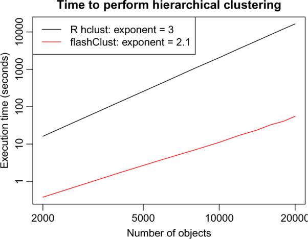
Execution time in seconds (y-axis) of hierarchical clustering as a function of the number of clustered objects n (x-axis). The black line represents the performance of the standard R function hclust, and the red line represents the performance of the function hclust implemented in the flashClust package. In the legend we also indicate the fitted exponents α of the model t = Cnnα, where t is the execution time and C is a constant.
We have packaged the original algorithm by Fionn Murtagh in the package flashClust which is available from the Comprehensive R Archive Network at http://CRAN.R-project.org/package=flashClust. The package flashClust implements a function hclust that is meant as a direct replacement of the standard R function hclust (package stats). In particular, the fast hclust takes the same arguments and returns the same results, only faster, as illustrated by the following example that uses a random distance matrix:
R> library(“flashClust”)
R> set.seed(1)
R> nNodes <- 2000
R> dst <- matrix(runif(n = nNodes^2, min = 0, max = 1), nNodes, nNodes)
R> system.time(h1 <- hclust(as.dist(dst), method = “average”))
| user | system | elapsed |
| 0.975 | 0.183 | 1.160 |
R> system.time(h2 <- stats∷hclust(as.dist(dst), method = “average”))
| user | system | elapsed |
| 29.452 | 0.230 | 29.733 |
The new flashClust::hclust function is much faster than the standard stats::hclust function. When clustering large data sets, the time savings attained by using flashClust are substantial. A timing example is provided in the script compareHClustSpeed.R included as supplementary material with this article. For example, clustering a relatively small data set of 4000 variables takes over 2 minutes using the standard R function hclust, whereas it takes less than 2 seconds using the hclust implemented in package flashClust. Clustering a large set of 20000 variables takes almost 4.6 hours using the standard R function hclust, whereas it takes less than 1 minute using the hclust implemented in package flashClust.
Supplementary Material
Acknowledgments
We would like to thank Lin Song, Daniel Müllner, and Chi Ming Yau for useful discussions. This work was supported by grants 1RC1 AG035610-01, 1U19AI063603-01, DE019255-01, DK072206, and P50CA092131.
References
- Ghazalpour A, Doss S, Zhang B, Wang S, Plaisier C, Castellanos R, Brozell A, Schadt EE, Drake TA, Lusis AJ, Horvath S. Integrating Genetic and Network Analysis to Characterize Genes Related to Mouse Weight. PLoS Genet. 2006;2(8):e130. doi: 10.1371/journal.pgen.0020130. doi:10.1371/journal.pgen.0020130. [DOI] [PMC free article] [PubMed] [Google Scholar]
- Hardin J, Mitani A, Hicks L, VanKoten B. A Robust Measure of Correlation between Two Genes on a Microarray. BMC Bioinformatics. 2007;8(1):220. doi: 10.1186/1471-2105-8-220. doi:10.1186/1471-2105-8-220. [DOI] [PMC free article] [PubMed] [Google Scholar]
- Hastie T, Tibshirani R, Friedman J. The Elements of Statistcal Learning: Data Mining, Inference, and Prediction. Springer-Verlag; 2001. [Google Scholar]
- Horvath S, Zhang B, Carlson M, Lu KV, Zhu S, Felciano RM, Laurance MF, Zhao W, Qi S, Chen Z, Lee Y, Scheck AC, Liau LM, Wu H, Geschwind DH, Febbo PG, Kornblum HI, Cloughesy TF, Nelson SF, Mischel PS. Analysis of Oncogenic Signaling Networks in Glioblastoma Identifies ASPM as a Novel Molecular Target. PNAS. 2006;103(46):17402–7. doi: 10.1073/pnas.0608396103. [DOI] [PMC free article] [PubMed] [Google Scholar]
- Kaufman L, Rousseeuw PJ. Finding Groups in Data: An Introduction to Cluster Analysis. John Wiley & Sons; 1990. [Google Scholar]
- Langfelder P, Horvath S. WGCNA: An R Package for Weighted Correlation Network Analysis. BMC Bioinformatics. 2008;9(1):559. doi: 10.1186/1471-2105-9-559. [DOI] [PMC free article] [PubMed] [Google Scholar]
- Langfelder P, Zhang B, Horvath S. Defining Clusters from a Hierarchical Cluster Tree: The Dynamic Tree Cut Package for R. Bioinformatics. 2007;24(5):719–20. doi: 10.1093/bioinformatics/btm563. [DOI] [PubMed] [Google Scholar]
- Lax DA. Robust Estimators of Scale: Finite-Sample Performance in Long-Tailed Symmetric Distributions. Journal of the American Statistical Association. 1985;80(391):736–741. [Google Scholar]
- Murtagh F. A Survey of Recent Advances in Hierarchical Clustering Algorithms. The Computer Journal. 1983;26(4):354–359. [Google Scholar]
- Murtagh F. Multivariate Data Analysis Software and Resources. The Classification Society. 2012 URL http://www.classification-society.org/csna/mda-sw/
- Ravasz E, Somera AL, Mongru DA, Oltvai ZN, Barabasi AL. Hierarchical Organization of Modularity in Metabolic Networks. Science. 2002;297(5586):1551–5. doi: 10.1126/science.1073374. [DOI] [PubMed] [Google Scholar]
- R Development Core Team . R: A Language and Environment for Statistical Computing. R Foundation for Statistical Computing; Vienna, Austria: 2011. ISBN 3-900051-07-0, URL http://www.R-project.org/ [Google Scholar]
- Whaley RC, Petitet A. Minimizing Development and Maintenance Costs in Supporting Persistently Optimized BLAS. Software: Practice and Experience. 2005;35(2):101–121. [Google Scholar]
- Wilcox RR. Introduction to Robust Estimation and Hypothesis Testing. 2nd edition Academic Press; 2005. [Google Scholar]
- Yip A, Horvath S. Gene Network Interconnectedness and the Generalized Topological Overlap Measure. BMC Bioinformatics. 2007;8(8):22. doi: 10.1186/1471-2105-8-22. [DOI] [PMC free article] [PubMed] [Google Scholar]
- Zhang B, Horvath S. General Framework for Weighted Gene Co-expression Analysis. Statistical Applications in Genetics and Molecular Biology. 2005;4(17) doi: 10.2202/1544-6115.1128. [DOI] [PubMed] [Google Scholar]
Associated Data
This section collects any data citations, data availability statements, or supplementary materials included in this article.