

Abstract
Motivation: There is growing momentum to develop statistical learning (SL) methods as an alternative to conventional genome-wide association studies (GWAS). Methods such as random forests (RF) and gradient boosting machine (GBM) result in variable importance measures that indicate how well each single-nucleotide polymorphism (SNP) predicts the phenotype. For RF, it has been shown that variable importance measures are systematically affected by minor allele frequency (MAF) and linkage disequilibrium (LD). To establish RF and GBM as viable alternatives for analyzing genome-wide data, it is necessary to address this potential bias and show that SL methods do not significantly under-perform conventional GWAS methods.
Results: Both LD and MAF have a significant impact on the variable importance measures commonly used in RF and GBM. Dividing SNPs into overlapping subsets with approximate linkage equilibrium and applying SL methods to each subset successfully reduces the impact of LD. A welcome side effect of this approach is a dramatic reduction in parallel computing time, increasing the feasibility of applying SL methods to large datasets. The created subsets also facilitate a potential correction for the effect of MAF using pseudocovariates. Simulations using simulated SNPs embedded in empirical data—assessing varying effect sizes, minor allele frequencies and LD patterns—suggest that the sensitivity to detect effects is often improved by subsetting and does not significantly under-perform the Armitage trend test, even under ideal conditions for the trend test.
Availability: Code for the LD subsetting algorithm and pseudocovariate correction is available at http://www.nd.edu/∼glubke/code.html.
Contact: glubke@nd.edu
Supplementary information: Supplementary data are available at Bioinformatics online.
1 INTRODUCTION
Genome-wide association studies (GWAS) have successfully detected numerous single-nucleotide polymorphisms (SNPs) associated with a variety of phenotypes, but the identified loci at best explain a modest proportion of the heritable variance estimated by twin and family studies (Manolio et al., 2009). Recent estimates of the heritable variance explained by all SNPs, however, indicate that genome-wide SNP data does offer substantial explanatory power (So et al., 2011; Yang et al., 2010). This gap of ‘missing heritability’ between heritability estimates and the SNPs detected by GWAS has led to increasing concern over the performance of GWAS, with attention focused on low power due to the multiple testing burden and small effect sizes, as well as the omission of rare disease alleles and epistatic effects, among other issues (Frazer et al., 2009; Maher, 2008; Moore, 2003; Park et al., 2010).
These shortcomings of GWAS have encouraged the application of statistical learning (SL) methods as an alternative for analyzing genome-wide data (Ayers and Cordell, 2010; He and Lin, 2011; Li et al., 2011a, b; Szymczak et al., 2009; Wang et al., 2011; Wu et al., 2010). SL methods are designed specifically for the task of identifying meaningful predictors in high-dimensional data, relying on data-driven algorithms rather than conventional parametric modeling. Numerous SL methods have been proposed for use with SNP data—including random forests (RF; Breiman, 2001), multifactor dimensionality reduction (Ritchie et al., 2001) and the lasso (Tibshirani, 1996)—generally with encouraging results.
RF has received significant attention in the genetics literature (Bureau et al., 2005; Garcia-Magarinos et al., 2009; Goldstein et al., 2010; Nonyane and Foulkes, 2008; Roshan et al., 2011; Wang et al., 2009) with surprisingly less attention given to gradient boosting machine (GBM; Friedman, 2001) despite its similarity to RF. Both RF and GBM build an ensemble of non-parametric prediction models, with each model constructed iteratively using all available SNPs. GBM additionally applies boosting to build each model with a focus of improving model fit for cases fit poorly in the previous iteration. Importantly, the iterative tree-building approach of RF and GBM accounts for conditional relationships and complex causal mechanisms, including epistasis and covariate effects, without a priori specification. Individual SNPs are then evaluated using variable importance measures, which quantify each SNP’s total contribution to the prediction of the phenotype (Breiman, 2001; Hastie et al., 2009). Such variable importance measures can be used to rank-order SNPs by importance, identifying potentially informative SNPs among genome-wide data.
Studies of RF with SNP data have yielded promising results. Simulations suggest that RF’s power to detect causal SNPs exceeds Fisher’s exact test when epistasis is present and is still comparable with Fisher’s exact test when detecting main effects only (Lunetta et al., 2004). RF maintains this advantage even if many noise SNPs are present (Bureau et al., 2005). Applying RF to genome-wide data is feasible, though computationally burdensome. With empirical genome-wide data, RF is capable of replicating GWAS results and identifying additional candidate SNPs (Goldstein et al., 2010).
Although these results are encouraging, further study is necessary to establish RF and GBM as viable alternatives to GWAS methods. Few studies of SL methods account for linkage disequilibrium (LD), utilize realistic effect sizes or compare the sensitivity of the SL method to GWAS. Roshan et al. (2011) considered more realistic LD and effect sizes but only focused on RF as a second-stage analysis. Meanwhile, GBM merits further consideration based on its strong performance relative to RF. Studies show GBM performs even better than RF for many data types (Caruana and Niculescu-Mizil, 2006; Hastie et al., 2009; Ogutu et al., 2011) but evaluation of its performance with genome-wide SNP data is still needed.
In addition, concerns have been raised about the impact of minor allele frequency (MAF) and LD on the variable importance measures used by RF and GBM to rank-order SNPs. With respect to LD, importance scores for correlated functional SNPs are inflated when using variable importance measures based on the Gini criterion (Strobl et al., 2008), whereas importance scores for functional SNPs correlated with uninformative predictors are deflated (Nicodemus and Malley, 2009). Correlated predictors do not induce bias in permutation-based importance measures, though the variability of importance scores is decreased (Nicodemus and Malley, 2009). MAF may also influence importance scores, with higher MAF being associated with higher Gini importance values for all SNPs, and higher permutation importance values for functional SNPs (Boulesteix et al., 2011). The influence of MAF may be attributed, at least in part, to the tendency of the RF algorithm to prefer predictors with higher variability (Strobl et al., 2007). Taken together, such effects may increase the difficulty of detecting disease-causing variants located in LD blocks or with low MAF, especially when using Gini-based importance measures.
Methods for controlling the impact of MAF and LD on variable importance have been proposed. To address the effect of LD, Meng et al. (2009) introduced a modified RF algorithm and accompanying importance measure that account for the competition between correlated SNPs for inclusion in RF models. Strobl et al. (2008) developed a conditional permutation scheme for the variable importance that successfully addresses the impact of correlated predictors. Alternatively, pseudocovariates (PCVs) may be added to the data to simultaneously address the effect of all structure in the data that are unrelated to the phenotype (Sandri and Zuccolotto, 2008, 2010).
Although each of these methods have been demonstrated to potentially reduce the impact of LD and MAF, all three increase the computational burden beyond what is feasible for genome-wide data. Meng et al. (2009) specifically note that their method does not scale to be feasible with genome-wide data. The current implementation of the conditional methods proposed by Strobl et al. (2008) also have substantially larger memory requirements than conventional RF. Correction with PCVs is similarly infeasible, effectively doubling the size of the data and requiring a number of replications of the analysis to establish stable estimates.
In sum, to establish RF and GBM as viable methods for genome-wide SNP data, it will be necessary (i) to address concerns over the impact of LD and MAF while maintaining computational feasibility and (ii) to provide a direct comparison with conventional GWAS methods under realistic conditions.
In this study, we propose and evaluate a procedure designed to reduce the impact of LD on RF, GBM or related SL methods for genome-wide data. The proposed method creates overlapping subsets of SNPs from a genome-wide dataset under the constraints that SNPs within a set are not in LD, and that each SNPs is represented in at least a user-specified number of subsets (see Methods). The SL method of choice can then be performed on the subsets without concern for LD, followed by an aggregation of results over subsets. Next, we show that the proposed subsetting procedure is computationally feasible for genome-wide data. Dividing the data into subsets makes analysis of each piece more manageable and facilitates parallel computation across multiple cores or on a high-performance grid for a drastic reduction of computing time. Third, we evaluate a correction for the impact of MAF adapted from the methods proposed by Sandri and Zuccolotto (2008, 2010), which is computationally feasible in combination with the subsetting procedure. Specifically, in each subset, we generate a small set of independent PCVs with zero association with the phenotype, coded as SNPs with MAF ranging from 0.01 to 0.50. Variable importance estimates for the PCVs in each subset are aggregated to provide a stable estimate of variable importance attributable to MAF. This estimate can then be used to correct the importances of the empirical SNPs. Finally, we provide a rigorous direct comparison of the sensitivity of RF and GBM to the Armitage trend test (ATT; Armitage, 1955), the test utilized most frequently in conventional GWAS analyses (McCarthy et al., 2008; Ziegler and Konig, 2010), under realistic data conditions. Using simulated SNPs embedded in empirical genetic data, we show that the sensitivity of RF and GBM is broadly consistent with the ATT for SNPs explaining as little as 1% of the phenotypic variance even under conditions that do not leverage the advantages of RF and GBM (i.e. a linear additive model without dominance or epistatic effects; Lunetta et al., 2004).
2 METHODS
2.1 RF/GBM analysis protocol
2.1.1 Random forests
RF is a machine learning algorithm that constructs classification or regression trees based on bootstrap samples of the data (Breiman, 2001). Samples not used to construct a given tree are the out-of-bag (OOB) sample. At each node A in a tree, a random subset of the predictors of size mtry is searched to find the predictor that partitions the data into the subsets that are most homogeneous with respect to the outcome variable. Thus for a case–control phenotype y, at a node A, the RF algorithm seeks the SNP with split s that maximizes the decrease in heterogeneity
| (1) |
where  and
and  are the left and right daughter nodes resulting from split s, P(A) is the probability of being placed in node A by split s, and
  is the Gini criterion
  (Hastie et al., 2009). The probabilities may be weighted based on a user-specified vector of prior probabilities classwt (Liaw and Wiener, 2002).
On the basis of the ensemble of trees, RF provides two measures of the importance of each SNP. The Gini importance measures the average value of Equation (1) in nodes split using a given SNP. The mean decrease in accuracy (MDA) importance is the average decrease in accuracy in classifying the OOB sample after permuting the given SNP (Breiman, 2002).
Analyses with RF were performed in R (R Development Core Team, 2011) using the randomForest package (Liaw and Wiener, 2002). Forests were grown to 5000 trees. The number of predictors attempted at each node, mtry, was set to 0.1 p, where p is the number of predictors in the data. These settings are consistent with the recommendations of Goldstein et al. (2010) for genome-wide data. In addition, prior probabilities (classwt) and voting thresholds (cuttoffs) were set equal to the case/control proportions for the observed phenotype in each analysis. All settings were chosen based on performance in pilot testing with real and simulated data (not shown).
2.1.2 Gradient boosting machine
GBM, like RF, is an ensemble method based on classification and regression trees constructed using bootstrap samples of the data. Unlike RF, however, each tree is fit to weighted residuals based on the previous trees in the ensemble. The contribution of each newly added tree to the prediction is limited by a shrinkage parameter. Similar to RF, variable importances are computed based on the average improvement in prediction from nodes split using a given SNP (Friedman, 2001).
Analyses with GBM were completed using the gbm package for R (Ridgeway, 2010). As with RF, the settings for GBM were based on pilot testing with empirical and simulated data. We used a 0.001 shrinkage parameter, 3000 trees and limited tree construction depth to first-order interactions.
2.2 LD subsetting algorithm
To reduce the effect of LD on variable importance, we propose an algorithm to select overlapping subsets of SNPs prior to analysis, such that the SNPs in each subset are in approximate linkage equilibrium and each SNP from the genome-wide data appears in at least a user-specified number of subsets. Subsequently, subsets are analyzed separately and results are aggregated.
The proposed algorithm creates subsets of SNPs from each chromosome, then combines these subsets to create genome-wide subsets. First, for chromosome c, let  be the
  data matrix of the
  SNPs on chromosome c ordered according to map location. To prevent order effects, begin by permuting the columns of
  within blocks of size b, where b is some small positive integer. In other words, randomly permute the order of columns 1 to b, columns b + 1 to
  of
of  to get the new data matrix
  .
.
To construct the zth subset for chromosome c, we first select the SNPs associated with columns  of
of  , where z and k are positive integers. Selecting k subsets in this way guarantees that every SNP in
  is selected once. Additional sets of k subsets can be constructed to ensure each SNP appears in a user-specified number of subsets, requiring s sets of k subsets to guarantee that each SNP is included in at least s subsets. The value of k is chosen by the researcher such that k – 2b is greater than the size (in number of SNPs) of the largest anticipated LD block in order to ensure that the SNPs in columns
  of
of  will not be in LD. The selection of k should be guided by using Haploview (Barrett et al., 2005) or other software to tag LD blocks in regions known to have the largest LD blocks (or the lowest recombination rate), and setting k slightly larger than the number of SNPs in the largest observed LD block.
Next, the subsets are augmented by adding additional SNPs that are in approximate linkage equilibrium with the initially selected SNPs, where linkage equilibrium is operationally defined by a user-specified maximum pairwise correlation t. These additional SNPs are selected by searching the intervals between the selected SNPs (e.g. columns 1 to  ). Within each interval, begin by removing from consideration SNPs that correlate above some correlation threshold t with the previously selected SNPs before or after the interval. For instance, for the interval from z + 1 to z + k – 1, SNPs correlated with the zth or z + kth SNPs, which have already been selected for subset z, are removed from consideration. For this study, we use a threshold of t= 0.1. Of the remaining SNPs, one SNP is randomly selected to be added to the zth subset. Any additional SNPs in the interval that correlate with the newly selected SNP greater than the threshold t are then removed from consideration. Continue randomly selecting SNPs in this way until no SNPs remain below the correlation threshold to be considered.
Once this procedure is finished, the zth subset for chromosome c is complete. The zth genome-wide subset is then defined by the union of the zth subset from each chromosome. Pseudocode summarizing the full algorithm is given in Figure 1. The desired SL method may then be run on each subset, and the importance of a given SNP is computed as its mean observed importance across subsets containing the SNP.
Fig. 1.
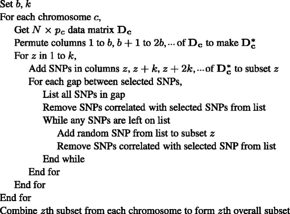
Pseudocode for the LD subsetting algorithm
2.3 Correction of importances with PCVs
Sandri and Zuccolotto (2010) proposed correcting variable importances by augmenting the data with PCVs, a second copy of the original predictor variables with the rows permuted to disrupt any association with the outcome variable while maintaining the structure among the predictors. The observed variable importance of the PCVs across a number of replications provides an estimate of the importance due to the structure of the predictors. The importance of each PCV can then be subtracted from the importance of the corresponding predictor to estimate the importance of the given predictor that is due to association with the outcome variable.
The LD subsetting algorithm does not itself address the issue of MAF but it does provide an opportunity to adapt the approach of Sandri and Zuccolotto (2010) to estimate and correct for the importance due to MAF while maintaining computational feasibility for genome-wide data. For each subset from the LD subsetting algorithm, independent PCVs are generated from  where the
  are evenly spaced on [0.01, 0.50] at intervals of 0.001 to fully capture the range of MAF values in GWAS data. These 491 PCVs are then appended to the subset of SNP data and analyzed with the selected SL method. After all subsets are analyzed, the importances are averaged to produce a single variable importance for each PCV.
Next, a loess regression curve is fit to the observed variable importances of the PCVs to estimate the expected importance at each MAF. The loess curve is selected to provide a smooth estimate without requiring specification of the non-linear relationship between MAF and variable importance (Supplementary Fig. S1). In this way, we obtain expected importances due to the effect of MAF only for MAF values in [0.01, 0.50].
The expected importance at each MAF can then be used to correct the importances that are observed when using RF or GBM. Specifically, for a given SNP with MAF m, subtract the expected importance at m, as estimated by the loess curve, from the observed importance for the SNP. The remaining importance for the SNP can be attributed to association with the phenotype.
Finally, to account for differences in the variability of the importance measure attributable to MAF, the corrected importance of the SNP is scaled by the standard deviation across subsets of the importance of the PCV with  closest to the MAF m. This is analogous to constructing a z statistic, with the PCVs providing an estimate of the mean and standard deviation for the null distribution of variable importances conditional on MAF. The resulting corrected variable importance may then be used to compare SNPs as usual.
Note that our proposed implementation of PCVs differs from Sandri and Zuccolotto (2010) on two key points. First, we generate PCVs as a small number of random binomial variables with varying MAFs, rather than using permuted rows from the data. This modification is justifiable because after LD subsetting the only known problematic structure in the data is variation in MAF. Second, we profit from the fact that we can include the small set of PCVs in each LD subset instead of having to perform multiple replications with the full data to get a stable estimate of the effect of MAF, allowing us to maintain computational feasibility for genome-wide data.
2.4 Embedding simulated SNP in empirical data
For this study of the impact of LD and MAF on variable importance, we simulate data for a SNP in LD with a range of MAF values. Specifically, we use an iterative procedure to simulate a SNP that correlates with an existing empirical SNP at a given correlation  and with a specified MAF. By embedding the simulated SNP in empirical SNP data, we are able to maintain a realistic data structure for the simulation studies. A different option would be to use one of the empirical SNPs and generate a phenotype value, but such an approach gives less control on LD and MAF and would require different locations of the target SNP for the different simulation settings.
To generate the simulated SNP, a continuous variable is generated first by adding noise drawn from  to an existing empirical SNP with complete data. Quantile thresholds based on the desired MAF, under the assumption of Hardy–Weinberg equilibrium, are applied to the continuous variable to create discrete SNP data. The correlation between the generated SNP and the existing SNP is controlled by adjusting
  for the noise. Decreasing
  increases LD with the empirical SNP, whereas increasing
  has the reverse effect. Adjustments to
  are made iteratively until the observed LD and MAF are within 0.01 of the desired values.
The possible correlation between a pair of SNPs is bounded by the difference in MAF. As a result, it is not possible to generate data for a wide range of values of MAF that still have a high correlation  with a single empirical SNP. Using formulas from Biswas and Hwang (2002), it is possible to establish the upper bound for
  at the population level for two SNPs with given MAFs. In finite samples, it is possible to achieve correlations that are somewhat higher than these bounds, but limitations are still present (Supplementary Information). As a result, some combinations of MAF and LD are omitted from simulations involving correlation with the empirical SNP, which has MAF m= 0.286, limiting the consideration of ρ = 0.9 to only simulated SNPs with MAF m= 0.3.
3 RESULTS
3.1 Evaluation of LD subsetting algorithm
As a baseline measurement of the impact of LD and MAF on variable importance in RF and GBM, both RF and GBM were used to analyze data containing a simulated SNP embedded in a 3000 SNP region of empirical data on N= 2235 individuals from a published study of hair morphology (Medland et al., 2009). An LD map of the 3000 empirical SNPs is shown in Supplementary Figure S2.
The simulated SNP was generated with one of four levels of LD (i.e. correlation ρ =0, 0.3, 0.6, 0.9 with the neighboring empirical SNP) and one of five levels of MAF (m= 0.05, 0.1, 0.2, 0.3, 0.5). LD and MAF levels were fully crossed, excluding conditions where data generation is not possible (see Methods). A case/control phenotype unrelated to the SNPs was generated with a probability 0.36 of being a case. Resulting variable importance measures from RF and GBM were collected for 250 replications for each combination of LD and MAF. Replications with invalid data generation were discarded.
Given a null phenotype, any observed systematic differences in variable importance can be attributed to MAF and to LD with the neighboring SNP. The effect of LD and MAF were tested using the non-parametric Kruskal–Wallis analysis of variance due to the skewed distribution of variable importances (Kruskal and Wallis, 1952). Significant results imply that the variable importances from the tested conditions do not have the same population distribution.
Replicating the findings of Boulesteix et al. (2011), a highly significant effect of MAF on the RF Gini importance of the simulated SNP is observed at each level of LD (Table 1). GBM produces very similar results. Although not previously established, the similarity of GBM importance measures to RF makes this result unsurprising.
Table 1.
Kruskal–Wallis test for the effect of LD and MAF on the variable importance of null SNPs
| Effect | Condition | df | RF Gini |
RF MDA |
GBM |
GBM + subsetting |
GBM + PCVs |
|||||
|---|---|---|---|---|---|---|---|---|---|---|---|---|
| x2 | P | x2 | P | x2 | P | x2 | P | x2 | P | |||
| MAF | ρ = 0.0 | 4 | 962.4 | <1 × 10⁻¹⁰ | 2.1 | 7.1 × 10⁻¹ | 148.0 | <1 × 10⁻¹⁰ | 381.7 | <1 × 10⁻¹⁰ | 18.5 | 9.8 × 10⁻⁴ |
| ρ = 0.3 | 4 | 1008.6 | <1 × 10⁻¹⁰ | 3.5 | 4.8 × 10⁻¹ | 222.6 | <1 × 10⁻¹⁰ | 399.7 | <1 × 10⁻¹⁰ | 8.8 | 6.6 × 10⁻² | |
| ρ = 0.6 | 4 | 1074.4 | <1 × 10⁻¹⁰ | 3.5 | 4.8 × 10⁻¹ | 206.1 | <1 × 10⁻¹⁰ | 355.1 | <1 × 10⁻¹⁰ | 22.7 | 1.5 × 10⁻⁴ | |
| LD | m = 0.05 | 2 | 342.8 | <1 × 10⁻¹⁰ | 21.2 | 2.5 × 10⁻⁵ | 2.8 | 2.5 × 10⁻¹ | 0.5 | 7.6 × 10⁻¹ | 0.1 | 9.5 × 10⁻¹ |
| m = 0.10 | 2 | 195.7 | <1 × 10⁻¹⁰ | 5.4 | 6.8 × 10⁻² | 3.1 | 2.1 × 10⁻¹ | 6.4 | 4.2 × 10⁻² | 0.7 | 7.1 × 10⁻¹ | |
| m = 0.20 | 2 | 162.0 | <1 × 10⁻¹⁰ | 1.8 | 4.2 × 10⁻¹ | 9.3 | 9.7 × 10⁻³ | 0.2 | 9.1 × 10⁻¹ | 0.7 | 7.2 × 10⁻¹ | |
| m = 0.30 | 3 | 596.0 | <1 × 10⁻¹⁰ | 26.3 | 8.3 × 10⁻⁶ | 52.4 | <1 × 10⁻¹⁰ | 1.6 | 6.6 × 10⁻¹ | 1.1 | 7.7 × 10⁻¹ | |
| m = 0.50 | 2 | 75.2 | <1 × 10⁻¹⁰ | 0.9 | 6.5 × 10⁻¹ | 0.1 | 9.6 × 10⁻¹ | 2.7 | 2.6 × 10⁻¹ | 2.7 | 2.6 × 10⁻¹ | |
Significance test results are given for uncorrected variable importances in RF and GBM, as well as for the GBM importance with LD subsetting and with PCVs. Results show the similar impact of MAF and LD on the RF Gini and GBM importances, the reduced effect of LD after subsetting, and the reduced effect of MAF after correction with PCVs. Tests are performed for the simple effect of MAF at a given LD ρ, and for the simple effect of LD at a given MAF m. With Bonferroni corrections for family-wise α= 0.05, P-values for the effect of MAF <1.7 × 10⁻², and P-values for the effect of LD <1 × 10⁻² indicate significant effects.
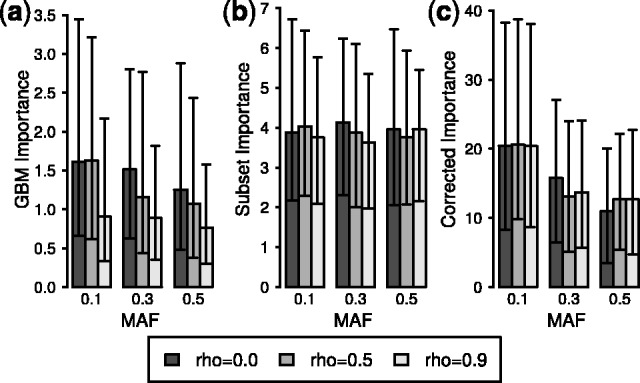
In addition, a highly significant effect of LD on the RF Gini importance is observed at each level of MAF. Strong effects for GBM and the RF MDA importance are also observed when m= 0.3 (Table 1). The observed effect is likely stronger here due to the inclusion of the higher LD condition ρ = 0.9, which can only be considered for MAF m= 0.3 due to the restrictions on correlation for binomial variables (see Methods). Plots of the median importance for GBM for each condition clearly suggest a trend toward a similar effect for other levels of MAF (Fig. 2a), though the corresponding Kruskal–Wallis tests are non-significant. Similar trends are observed for RF (Supplementary Figs S3a and S4a).
Fig. 2.
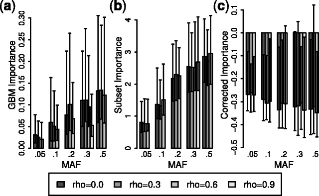
Median observed GBM variable importance by LD and MAF. Observed median importance is shown for GBM with (a) no correction, (b) LD subsetting and (c) LD subsetting and PCVs. The skewed distribution of importances makes SEs uninformative, so error bars instead indicate observed upper and lower quartiles. Differences within a value of MAF suggest an effect of LD, and differences at a correlation ρ suggest an effect of MAF
3.1.1 Improvement from LD subsetting algorithm
Applying the proposed LD subsetting algorithm to the simulated data with s= 1 set of k= 300 subsets results in a drastic reduction in the effect of LD on the resulting aggregated importances for GBM and RF. Importantly, the process of aggregating results from the subsets does not favor any given SNPs based on the number of subsets containing the SNP (Supplementary Information). After correcting for multiple testing, the Kruskal–Wallis test shows no significant effect of LD for GBM. Note also that large effects of MAF are still observed (Table 1). The improvement due to subsetting is especially evident at the m= 0.30 level. Plots of the median variable importance in each condition similarly show no systematic trend related to LD (Fig. 2b). Dramatic improvements are also observed for RF (Supplementary Table S1 and Figs S3b and S4b).
3.2 Impact on computational feasibility
In addition to reducing the effect of LD, the LD subsetting algorithm facilitates distribution of the analysis across a grid environment. For example, using a single core on a server with Dual Six-Core AMD Opteron Model 2431 CPUs, RF requires over 19 h and 3.5 GB of RAM to complete an analysis of chromosome 22 from the complete empirical data (30 218 SNPs). In contrast, the subsets created by the subsetting algorithm can each be analyzed with RF with 1.3 GB of RAM in ∼44 min. Creating the subsets themselves requires 30 min and 1.8 GB of RAM, and negligible resources are required to aggregate the final results. If a grid environment is available to process 50 of the k= 300 subsets in parallel, using LD subsets with RF yields a 75% reduction in the time required to complete the analysis, and a 49% reduction in the maximum RAM required. Even greater reductions are observed for GBM, shrinking the computational burden from 10 h and 4.3 GB of RAM for the full chromosome to 7 min and 0.5 GB of RAM per subset, yielding a 57% reduction in the maximum RAM requirement and a 89% reduction in total computing time in a grid environment with 50 parallel cores. Supplementary Table S2 details these results.
3.3 Addition of PCVs
The subsets created by the LD subsetting algorithm offer an opportunity to include PCVs. Since there are  50 000 SNPs in each subset when 300 subsets are produced for genome-wide data containing
  2 million SNPs, 491 PCVs are a modest addition with a negligible impact on the computational burden.
Given the similar performance of RF and GBM, and the larger computational burden of RF, we focus on evaluating PCVs with GBM. Table 1 reports the results of 250 replications of GBM with the PCV correction. Although a significant effect of MAF remains at ρ = 0 and ρ = 0.6, the magnitude of the effect is drastically reduced (Fig. 2c). Note that the negative GBM importances are an artifact of the positively skewed distribution of importances; using PCVs to center the mean importance of a SNP with no effect at zero yields a negative median for the skewed distribution. SNPs with a true effect are still expected to have positive importances (see Section 3.4).
3.4 Sensitivity to functional SNPs
The results thus far show a reduction of the influence of LD and MAF on the variable importance for SNPs with no association with the phenotype. To model the effect of LD and MAF on variable importance for functional SNPs, three sets of 28 simulated SNPs were embedded in the 3000 SNP region used previously. The three sets were generated with MAF m= 0.1, 0.3 and 0.5, respectively, and embedded avoiding disruption of LD blocks in the empirical data.
Each set of 28 SNPs contains three LD blocks of four SNPs each with ρ = 0.9, three LD blocks with ρ = 0.5 and one block with ρ = 0. The LD and MAF conditions used here differ from the previous simulation to provide a less complex setting while still covering a full range of LD and MAF values. Among the 28 simulated SNPs, there are six functional SNPs, jointly explaining 9% of the variance in a continuous outcome variable, which is then dichotomized to a case/control phenotype. Specifically, within each set of SNPs, x1, … , x28, SNPs x1, x13 and x25, each explain 2% of the variance in the continuous outcome, and x5, x17 and x26 each explain 1% of the variance (Supplementary Fig. S5). This design fully crosses effect size by LD within each set of 28 SNPs, crossed by MAF for the three sets.
We focus our analysis on the functional SNPs with the more realistic effect size of 1% variance explained (x5, x17 and x26). Results for tag SNPs and the remaining functional SNPs are available in the Supplementary Information. In addition to testing the effect of MAF and LD on the resulting variable importances, we also consider the sensitivity of each method to identify functional SNPs. Since RF and GBM do not include formal significance testing, we define the detection rate as the proportion of replications in which the observed importance for a given functional SNP exceeds the highest observed importance among the simulated non-effect SNPs.
3.4.1 Uncorrected RF and GBM
To again establish a baseline, variable importances from RF and GBM were collected for 250 replications without the LD subsetting algorithm or PCVs. Figure 3a illustrates the resulting median GBM importance values for the simulated SNPs (for RF see Supplementary Figs S6a and S7a). Comparing the three functional SNPs suggests a strong effect of LD, with lower importance given to the SNPs in strong LD. The effect of LD is significant for GBM and the RF Gini importance according to the Friedman test and approaches significance for the RF MDA importance (Table 2). The Friedman test, a non-parametric equivalent of the repeated measures analysis of variance, is applied here due to the skewed distribution of the importances and the dependence among the importances of SNPs together in a replication (Friedman, 1937).
Fig. 3.
GBM variable importance for functional SNPs. Median GBM variable importance using (a) uncorrected importance, (b) LD subsetting and (c) LD subsetting with PCVs. The skewed distribution of importances makes SEs uninformative, so error bars instead indicate observed upper and lower quartiles. Comparison of the plots shows the reduced impact of LD after LD subsetting and the increased impact of MAF when including PCVs
Table 2.
Friedman test for effect of LD and MAF on the variable importance of functional SNPs
| Effect | Condition | RF Gini |
RF MDA |
GBM |
GBM + subsetting |
GBM + PCVs |
|||||
|---|---|---|---|---|---|---|---|---|---|---|---|
| x2 | P | x2 | P | x2 | P | x2 | p | x2 | p | ||
| MAF | ρ = 0.9 | 11.9 | 2.6 × 10⁻³ | 7.0 | 3.0 × 10⁻² | 1.7 | 4.2 × 10⁻¹ | 0.6 | 7.5 × 10⁻¹ | 21.5 | 2.1 × 10⁻⁵ |
| ρ = 0.5 | 13.8 | 1.0 × 10⁻³ | 7.0 | 3.0 × 10⁻² | 7.9 | 1.9 × 10⁻² | 2.3 | 3.1 × 10⁻¹ | 21.8 | 1.9 × 10⁻⁵ | |
| ρ = 0.0 | 14.6 | 6.8 × 10⁻⁴ | 13.3 | 1.3 × 10⁻³ | 1.1 | 5.7 × 10⁻¹ | 1.5 | 4.7 × 10⁻¹ | 44.2 | 2.5 × 10⁻¹⁰ | |
| LD | m = 0.1 | 17.6 | 1.5 × 10⁻⁴ | 1.0 | 6.1 × 10⁻¹ | 17.7 | 1.4 × 10⁻⁴ | 1.4 | 5.0 × 10⁻¹ | 0.5 | 7.8 × 10⁻¹ |
| m = 0.3 | 32.0 | 1.1 × 10⁻⁷ | 0.5 | 8.0 × 10⁻¹ | 17.7 | 1.4 × 10⁻⁴ | 6.5 | 3.9 × 10⁻² | 0.7 | 6.9 × 10⁻¹ | |
| m = 0.5 | 12.7 | 1.7 × 10⁻³ | 5.0 | 8.2 × 10⁻² | 19.6 | 5.6 × 10⁻⁵ | 0.3 | 8.4 × 10⁻¹ | 4.5 | 1.0 × 10⁻¹ | |
Tests are performed for the simple effect of MAF at a given LD ρ, and for the simple effect of LD at a given MAF m. All tests have df= 2. With Bonferroni corrections for family-wise α= 0.05, P-values <1.7 × 10⁻² indicate significant effects.
The results also seem to suggest a modest effect of MAF for each functional SNP, but the effect is only significant for the RF Gini importance. Unexpectedly, lower variable importance is observed for functional SNPs with high MAF (Fig. 3a) compared with the higher importance observed for null SNPs with high MAF (Fig. 2a). Further analysis, however, suggests this is an artifact of the differing magnitude of the regression coefficients required to maintain equal effect sizes while varying MAF (Supplementary Information).
Table 3 reports the detection rates for GBM, along with exact 95% confidence intervals for the proportion as defined by Clopper and Pearson (1934). Corresponding results for RF are reported in Supplementary Table S3. The raw values are of little interest but yield a basis for comparison with other methods.
Table 3.
Functional SNP detection rate by method, LD ρ, and MAF m
| m | Method | Detection rate (95% confidence interval) |
||
|---|---|---|---|---|
| ρ = 0.9 | ρ = 0.5 | ρ = 0 | ||
| 0.1 | GBM | 0.79 (0.74–0.84) | 0.86 (0.81–0.90) | 0.89 (0.85–0.93) |
| GBM Sub | 0.88 (0.84–0.92) | 0.90 (0.86–0.93) | 0.85 (0.80–0.89) | |
| GBM PCV | 0.88 (0.84–0.92) | 0.92 (0.88–0.95) | 0.87 (0.82–0.91) | |
| ATT | 0.90 (0.86–0.94) | 0.92 (0.88–0.95) | 0.94 (0.90–0.97) | |
| 0.3 | GBM | 0.80 (0.74–0.88) | 0.82 (0.76–0.86) | 0.88 (0.84–0.92) |
| GBM Sub | 0.88 (0.83–0.91) | 0.89 (0.84–0.92) | 0.87 (0.82–0.91) | |
| GBM PCV | 0.83 (0.78–0.88) | 0.81 (0.76–0.86) | 0.86 (0.82–0.90) | |
| ATT | 0.92 (0.88–0.95) | 0.92 (0.88–0.95) | 0.90 (0.85–0.93) | |
| 0.5 | GBM | 0.78 (0.72–0.83) | 0.83 (0.78–0.88) | 0.85 (0.80–0.89) |
| GBM Sub | 0.87 (0.82–0.91) | 0.86 (0.81–0.90) | 0.84 (0.79–0.89) | |
| GBM PCV | 0.84 (0.79–0.89) | 0.82 (0.76–0.86) | 0.77 (0.71–0.82) | |
| ATT | 0.90 (0.86–0.94) | 0.93 (0.89–0.96) | 0.94 (0.90–0.96) | |
‘Detection’ in each replication is defined as importance (or test statistic) for a functional SNP greater than the highest observed importance among simulated SNPs unassociated with the phenotype. Results are given for the ATT, uncorrected GBM importance, GBM with LD subsetting, and GBM with PCVs, showing that in most cases the detection rate for GBM-based methods is within sampling error of the ATT. Proportions are out of 250 replications. Values in bold have confidence intervals that overlap the confidence interval for the detection rate of the ATT.
3.4.2 LD subsetting algorithm
As observed for null SNPs, introducing LD subsetting reduces the impact of LD on variable importance for functional SNPs (Fig. 3b). With LD subsetting, the effect of LD on variable importance is non-significant after correction for multiple testing (Table 2). LD subsetting also increases the relative importance of tag SNPs in LD with a functional SNP, reducing the downward pressure on the importance of SNPs in a strong LD block (Supplementary Fig. S8). Similar results are observed for RF (Supplementary Table S4).
Investigation of the detection rates for GBM with and without LD subsetting shows LD subsetting markedly improves detection of the functional SNPs in LD blocks. In exchange, there is a modest decrease in the detection rate for SNPs not in LD, especially at low MAF (Table 3). For RF, LD subsetting improves detection rates for the MDA importance but significantly impairs detection of functional SNPs with low MAF when using the Gini importance (Supplementary Table S3), likely due a strengthened effect of MAF.
3.4.3 PCV correction
Although the effect of MAF on the importance of effect SNPs after LD subsetting is non-significant (Table 2), the inclusion of PCVs to correct for MAF may still be desirable to at least partially address the impact of MAF on the importance of null SNPs. As before, the computational burden of RF leads us to focus on the results for GBM.
Figure 3c depicts the resulting GBM variable importances after inclusion of PCVs. Although the effect of LD remains non-significant, there is a strong, significant effect of MAF on the importances (Table 2). This result is unsurprising given that the trend of GBM variable importances associated with MAF works in the opposite direction for functional SNPs compared with non-effect SNPs. By adjusting the importance to account for the inflated importance of non-effect SNPs with high MAF, the PCV correction strengthens the trend toward lower importance for functional SNPs with high MAF values. As before, the resulting trend in variable importances may be interpreted as reflecting the magnitude of regression coefficients rather than a direct effect of MAF (see Supplementary Information).
The impact of including PCVs on the detection rate is more limited. Analyses using GBM with PCVs show slightly higher detection rates for SNPs with low MAF, and a moderate decrease in detection rates for SNPs with higher MAF, but the difference is generally within sampling variation (Table 3).
3.4.4 Armitage trend test
To establish the usefulness of SL methods for genome-wide data, it is important to compare their performance to conventional methods. Since the current simulations rely on the same additive genetic model assumed by the ATT, we do not anticipate that RF and GBM will provide any improvement over the detection rate of the ATT. Instead, we hope to show that even under ideal circumstances for the ATT, little sensitivity is lost by using RF and GBM, such that RF and GBM may improve sensitivity to epistatic and non-additive effects without substantial sacrifices of sensitivity to additive effects.
Comparison of the detection rates for GBM with the ATT indicates that in most conditions the difference between the two methods is within the range of sampling variation, especially when LD subsetting is used (Table 3). Indeed, there is a strong visual similarity between the pattern of observed P-values for the ATT and the corresponding variable importances from GBM with LD subsetting (Supplementary Figs S8b and S9). Results for RF are somewhat weaker (Supplementary Table S3). Note that in order to maintain a fair comparison, we define detection for the ATT by treating the test statistic as an analog to the variable importance rather than requiring statistical significance. In sum, it appears GBM, with the aid of LD subsetting, does not substantially under-perform the ATT, even under ideal circumstances for the ATT.
4 DISCUSSION
SL methods such as RF and GBM are a viable alternative to conventional parametric testing of individual SNPs in a GWAS. However, there are valid concerns over the impact of LD and MAF on variable importance measures that must be addressed. In response, this study presents an integrated approach to meaningfully reduce the effect of LD and MAF on variable importance in RF and GBM.
The results of this study show that the proposed subsetting algorithm can successfully reduce or eliminate the effect of LD on the variable importance measures of RF and GBM. The process of aggregating results over the subsets is not biased by the number of subsets containing a given SNP and, in many cases, may aid the detection of effect SNPs. In particular, the use of LD subsetting can be expected to aid RF and GBM is identifying effect SNPs within LD blocks. Since LD subsets are constructed prior to analysis, the procedure could also be applied to other SL methods.
Importantly, GBM provides detection rates for the functional SNPs within sampling variation of detection rates for the ATT. This result for GBM is especially encouraging given that this study uses an additive genetic model that precisely matches the type of effect anticipated by the ATT. SL methods may be expected to provide substantial improvement over the ATT for detecting correlated effect SNPs and SNPs with non-additive and epistatic effects (Garcia-Magarinos et al., 2009). Alternatively, RF and GBM may act as an initial screen to reduce genome-wide data to a set of candidate SNPs small enough to make thorough modeling of their complex relationships feasible using penalized regression or other appropriate methods (Ayers and Cordell, 2010).
The LD subsetting approach also facilitates the introduction of PCVs, as proposed by Sandri and Zuccolotto (2010), which may potentially be used to correct for the effect of MAF on variable importance measures. The proposed PCV correction evaluated in this study provides a marked reduction in the effect of MAF on non-effect SNPs. Caution is necessary in applying PCVs, however, given a moderate effect of MAF remains and the effect of MAF on the importance of functional SNPs may be magnified, with uncertain implications (Supplementary Information). Still, PCVs at minimum provide the option of emphasizing sensitivity to SNPs with low MAF, which may contain the majority of heritable variance for some phenotypes, such as high-density lipoprotein (HDL) cholesterol (Park et al., 2011), and can be difficult to detect with conventional methods (Wang et al., 2005). Finally, in addition to PCVs numerous covariates for comorbid disorders, environmental factors and other influential variables may be included in the analysis with a much lower computational cost than for popular GWAS software (Shabalin, 2012).
A number of factors may be considered in seeking to improve the approaches evaluated by this study. More careful tuning of the metaparameters for the LD subsetting algorithm, including the selection of k, b and t, may enhance the effectiveness of the correction. Alternative methods to improve the use of PCVs to correct for the effect of MAF may also be explored. The correction proposed here is only one possible application of PCVs; other versions may improve the effectiveness of PCVs or carry different advantages tailored to the preferences of the researcher. Finally, these results show strong results for GBM that are consistent with the more widely known RF; additional work should be performed to evaluate GBM as a viable tool for analyzing genome-wide data, especially given its lighter computational burden.
Although our approach does not fully eliminate the impact of LD and MAF on variable importance measures, the proposed corrections provide a satisfying improvement. Importantly, LD subsetting also facilitates analysis in a parallel environment, improving the computational feasibility of these methods for genome-wide data. Continuing efforts to establish the validity, reliability and feasibility of SL methods such as RF and GBM with genome-wide data will be crucial to establishing these methods as viable alternatives to conventional GWAS analyses.
Supplementary Material
ACKNOWLEDGMENTS
We are grateful for the assistance of Drs Sarah Medland and Nicholas Martin who kindly permitted us to use the empirical genotype data from their study of hair morphology.
Funding: US National Institutes of Health (DA018673 to G.H.L.). Data collection for the hair morphology study supported by the Australian National Health and Medical Research Council (241944, 339462, 389927, 89875, 389891, 389892, 389938, 442915, 442981, 496739, 552485 and 552498), the Australian Research Council (A7960034, A79906588, A79801419, DP0770096, DP0212016 and DP0343921), the FP-5 GenomEUtwin Project (QLG2-CT-2002-01254) and the US National Institutes of Health (AA07535, AA10248, AA13320, AA13321, AA13326, AA14041 and MH66206).
Conflict of Interest: none declared.
REFERENCES
- Armitage P. Tests for linear trends in proportions and frequencies. Biometrics. 1955;11:375–386. [Google Scholar]
- Ayers K.L., Cordell H.J. SNP selection in genome-wide and candidate gene studies via penalized logistic regression. Genet. Epidemiol. 2010;34:879–891. doi: 10.1002/gepi.20543. [DOI] [PMC free article] [PubMed] [Google Scholar]
- Barrett J.C., et al. Haploview: analysis and visualization of LD and haplotype maps. Bioinformatics. 2005;21:263–265. doi: 10.1093/bioinformatics/bth457. [DOI] [PubMed] [Google Scholar]
- Biswas A., Hwang J. A new bivariate binomial distribution. Stat. Probab. Lett. 2002;60:231–240. [Google Scholar]
- Boulesteix A., et al. Random forest Gini importance favours SNPs with large minor allele frequency: impact, sources and recommendations. Brief. Bioinform. 2011;13:292–304. doi: 10.1093/bib/bbr053. [DOI] [PubMed] [Google Scholar]
- Breiman L. Random forests. Mach. Learn. 2001;45:5–32. [Google Scholar]
- Breiman L. (2002). Manual on setting up, using, and understanding random forests v3.1. http://oz.berkeley.edu/users/breiman/Using_random_forests_V3.1.pdf.
- Bureau A., et al. Identifying SNPs predictive of phenotype using random forests. Genet. Epidemiol. 2005;28:171–182. doi: 10.1002/gepi.20041. [DOI] [PubMed] [Google Scholar]
- Caruana R., Niculescu-Mizil A. An empirical comparison of supervised learning algorithms.. Proceedings of the 23rd International Conference on Machine Learning (ICML’06). ACM, New York.2006. [Google Scholar]
- Clopper C., Pearson E. The use of confidence or fiducial limits illustrated in the case of the binomial. Biometrika. 1934;26:404–413. [Google Scholar]
- Frazer K.A., et al. Human genetic variation and its contribution to complex traits. Nat. Rev. Genet. 2009;10:241–251. doi: 10.1038/nrg2554. [DOI] [PubMed] [Google Scholar]
- Friedman J.H. Greedy function approximation: a gradient boosting machine. Ann. Statist. 2001;29(5):1189–1232. [Google Scholar]
- Friedman M. The use of ranks to avoid the assumption of normality implicit in the analysis of variance. J. Am. Stat. Ass. 1937;32(200):675–701. [Google Scholar]
- Garcia-Magarinos M., et al. Evaluating the ability of tree-based methods and logistic regression for the detection of SNP-SNP interaction. Ann. Hum. Genet. 2009;73:360–369. doi: 10.1111/j.1469-1809.2009.00511.x. [DOI] [PubMed] [Google Scholar]
- Goldstein B.A., et al. An application of random forests to a genome-wide association dataset: methodological considerations & new findings. BMC Genet. 2010;11:49. doi: 10.1186/1471-2156-11-49. [DOI] [PMC free article] [PubMed] [Google Scholar]
- Hastie T., et al. The Elements of Statistical Learning: Data Mining, Inference, and Prediction. 2nd. 2009. Springer, New York. [Google Scholar]
- He Q., Lin D. A variable selection method for genome-wide association studies. Bioinformatics. 2011;27(1):1–8. doi: 10.1093/bioinformatics/btq600. [DOI] [PMC free article] [PubMed] [Google Scholar]
- Kruskal W.H., Wallis W.A. Use of ranks in one-criterion variance analysis. J. Am. Stat. Ass. 1952;47:583–621. [Google Scholar]
- Li J., et al. The Bayesian lasso for genome-wide association studies. Bioinformatics. 2011a;27:516–523. doi: 10.1093/bioinformatics/btq688. [DOI] [PMC free article] [PubMed] [Google Scholar]
- Li J., et al. Detecting epistatic effects in association studies at a genomic level based on an ensemble approach. Bioinformatics. 2011b;27:i222–i229. doi: 10.1093/bioinformatics/btr227. [DOI] [PMC free article] [PubMed] [Google Scholar]
- Liaw A., Wiener M. Classification and regression by randomForest. R News. 2002;2:18–22. [Google Scholar]
- Lunetta K.L., et al. Screening large-scale association study data: exploiting interactions using random forests. BMC Genet. 2004;5:32. doi: 10.1186/1471-2156-5-32. [DOI] [PMC free article] [PubMed] [Google Scholar]
- Maher B. Personal genomes: the case of the missing heritability. Nature. 2008;456:18–21. doi: 10.1038/456018a. [DOI] [PubMed] [Google Scholar]
- Manolio T.A., et al. Finding the missing heritability of complex diseases. Nature. 2009;461:747–753. doi: 10.1038/nature08494. [DOI] [PMC free article] [PubMed] [Google Scholar]
- McCarthy M.I., et al. Genome-wide association studies for complex traits: consensus, uncertainty and challenges. Nat. Rev. Genet. 2008;9:356–369. doi: 10.1038/nrg2344. [DOI] [PubMed] [Google Scholar]
- Medland S., et al. Common variants in the Trichohyalin gene are associated with straight hair in Europeans. Am. J. Hum. Genet. 2009;85:750–755. doi: 10.1016/j.ajhg.2009.10.009. [DOI] [PMC free article] [PubMed] [Google Scholar]
- Meng Y.A., et al. Performance of random forest when SNPs are in linkage disequilibrium. BMC Bioinformatics. 2009;10:78. doi: 10.1186/1471-2105-10-78. [DOI] [PMC free article] [PubMed] [Google Scholar]
- Moore J.H. The ubiquitous nature of epistasis in determining susceptibility to common human diseases. Hum. Hered. 2003;56:73–82. doi: 10.1159/000073735. [DOI] [PubMed] [Google Scholar]
- Nicodemus K.K., Malley J.D. Predictor correlation impacts machine learning algorithms: implications for genomic studies. Bioinformatics. 2009;25:1884–1890. doi: 10.1093/bioinformatics/btp331. [DOI] [PubMed] [Google Scholar]
- Nonyane B., Foulkes A.S. Application of two machine learning algorithms to genetic association studies in the presence of covariates. BMC Genet. 2008;9:71. doi: 10.1186/1471-2156-9-71. [DOI] [PMC free article] [PubMed] [Google Scholar]
- Ogutu J.O., et al. A comparison of random forests, boosting and support vector machines for genomic selection. BMC Proc. 2011;5(Suppl 3):S11. doi: 10.1186/1753-6561-5-S3-S11. [DOI] [PMC free article] [PubMed] [Google Scholar]
- Park J., et al. Estimation of effect size distribution from genome-wide association studies and implications for future discoveries. Nat. Genet. 2010;42:570–575. doi: 10.1038/ng.610. [DOI] [PMC free article] [PubMed] [Google Scholar]
- Park J., et al. Distribution of allele frequencies and effect sizes and their interrelationships for common genetic susceptibility variants. Proc. Natl Acad. Sci. U.S.A. 2011;108:18026–18031. doi: 10.1073/pnas.1114759108. [DOI] [PMC free article] [PubMed] [Google Scholar]
- R Development Core Team. R: A Language and Environment for Statistical Computing. 2011. R Foundation for Statistical Computing, Vienna, Austria. [Google Scholar]
- Ridgeway G. GBM: Generalized boosted regression models. 2010. R package version 1.6-3.1. [Google Scholar]
- Ritchie M.D., et al. Multifactor-dimensionality reduction reveals high-order interactions among estrogen-metabolism genes in sporadic breast cancer. Am. J. Hum. Genet. 2001;69:138–147. doi: 10.1086/321276. [DOI] [PMC free article] [PubMed] [Google Scholar]
- Roshan U., et al. Ranking causal variants and associated regions in genome-wide association studies by the support vector machine and random forest. Nucleic Acids Res. 2011;39:e62. doi: 10.1093/nar/gkr064. [DOI] [PMC free article] [PubMed] [Google Scholar]
- Sandri M., Zuccolotto P. A bias correction algorithm for the Gini variable importance measure in classification trees. J. Comp. Graph. Stat. 2008;17:611–628. [Google Scholar]
- Sandri M., Zuccolotto P. Analysis and correction of bias in total decrease in node impurity measures for tree-based algorithms. Stat Comput. 2010;20:393–407. [Google Scholar]
- Shabalin A.A. Matrix eQTL: ultra fast eQTL analysis via large matrix operations. Bioinformatics. 2012;28:1353–1358. doi: 10.1093/bioinformatics/bts163. [DOI] [PMC free article] [PubMed] [Google Scholar]
- So H., et al. Uncovering the total heritability explained by all true susceptibility variants in a genome-wide association study. Genet. Epidemiol. 2011;35:447–456. doi: 10.1002/gepi.20593. [DOI] [PubMed] [Google Scholar]
- Strobl C., et al. Bias in random forest variable importance measures: illustrations, sources and a solution. BMC Bioinform. 2007;8:25. doi: 10.1186/1471-2105-8-25. [DOI] [PMC free article] [PubMed] [Google Scholar]
- Strobl C., et al. Conditional variable importance for random forests. BMC Bioinform. 2008;9:307. doi: 10.1186/1471-2105-9-307. [DOI] [PMC free article] [PubMed] [Google Scholar]
- Szymczak S., et al. Machine learning in genome-wide association studies. Genet. Epidemiol. 2009;33(Suppl 1):S51–S57. doi: 10.1002/gepi.20473. [DOI] [PubMed] [Google Scholar]
- Tibshirani R. Regression shrinkage and selection via the lasso. J. R. Stat. Soc. Ser. B. 1996;58:267–288. [Google Scholar]
- Wang M., et al. Detecting significant single-nucleotide polymorphisms in a rheumatoid arthritis study using random forests. BMC Proc. 2009;3(Suppl 7):S69. doi: 10.1186/1753-6561-3-s7-s69. [DOI] [PMC free article] [PubMed] [Google Scholar]
- Wang W.Y., et al. Genome-wide association studies: theoretical and practical concerns. Nat. Rev. Genet. 2005;6:109–118. doi: 10.1038/nrg1522. [DOI] [PubMed] [Google Scholar]
- Wang Y., et al. An empirical comparison of several recent epistatic interaction detection methods. Bioinformatics. 2011;27:2936–2943. doi: 10.1093/bioinformatics/btr512. [DOI] [PubMed] [Google Scholar]
- Wu J., et al. Screen and clean: a tool for identifying interactions in genome-wide association studies. Genet. Epidemiol. 2010;34:275–285. doi: 10.1002/gepi.20459. [DOI] [PMC free article] [PubMed] [Google Scholar]
- Yang J., et al. Common SNPs explain a large proportion of the heritability for human height. Nat. Genet. 2010;42:565–571. doi: 10.1038/ng.608. [DOI] [PMC free article] [PubMed] [Google Scholar]
- Ziegler A., Konig I.R. A Statistical Approach to Genetic Epidemiology: Concepts and Applications. 2nd. Weinheim, Germany: Wiley-VCH; 2010. [Google Scholar]
Associated Data
This section collects any data citations, data availability statements, or supplementary materials included in this article.