The role of fine-scale anatomical structure in the dynamics of reentry in computational models of the rabbit ventricles

Abstract

Fine-scale anatomical structures in the heart may play an important role in sustaining cardiac arrhythmias. However, the extent of this role and how it may differ between species are not fully understood. In this study we used computational modelling to assess the impact of anatomy upon arrhythmia maintenance in the rabbit ventricles. Specifically, we quantified the dynamics of excitation wavefronts during episodes of simulated tachyarrhythmias and fibrillatory arrhythmias, defined as being respectively characterised by relatively low and high spatio-temporal disorganisation. Two computational models were used: a highly anatomically detailed MR-derived rabbit ventricular model (representing vasculature, endocardial structures) and a simplified equivalent model, constructed from the same MR-data but lacking such fine-scale anatomical features. During tachyarrhythmias, anatomically complex and simplified models showed very similar dynamics; however, during fibrillatory arrhythmias, as activation wavelength decreased, the presence of fine-scale anatomical details appeared to marginally increase disorganisation of wavefronts during arrhythmias in the complex model. Although a small amount of clustering of reentrant rotor centres (filaments) around endocardial structures was witnessed in follow-up analysis (which slightly increased during fibrillation as rotor size decreased), this was significantly less than previously reported in large animals. Importantly, no anchoring of reentrant rotors was visibly identifiable in arrhythmia movies. These differences between tachy- and fibrillatory arrhythmias suggest that the relative size of reentrant rotors with respect to anatomical obstacles governs the influence of fine-scale anatomy in the maintenance of ventricular arrhythmias in the rabbit. In conclusion, our simulations suggest that fine-scale anatomical features play little apparent role in the maintenance of tachyarrhythmias in the rabbit ventricles and, contrary to experimental reports in larger animals, appear to play only a minor role in the maintenance of fibrillatory arrhythmias. These findings also have important implications in optimising the level of detail required in anatomical computational meshes frequently used in arrhythmia investigations.

Key points

• The specific mechanisms by which fine-scale structures within the heart may interact with complex excitation wavefronts during cardiac arrhythmias to increase their stability, and how this interaction may differ between species are currently incompletely understood.

• Computational models provide an important basic science tool in mechanistic arrhythmia enquiry. Recent advances in cardiac imaging have allowed the generation of highly anatomically detailed computational ventricular models including fine-scale features such as blood vessels and endocardial structures.

• Using such an anatomically detailed MR-derived rabbit ventricular model, in conjunction with a simplified equivalent model, we assessed the role played by fine-scale anatomy in the sustenance of different types of simulated arrhythmias.

• Our simulation results suggest that, in the rabbit, anatomical structures such as the vasculature and endocardial structures play little role in the maintenance of cardiac arrhythmias, although their role becomes marginally more important with increasing arrhythmia complexity.

• Consequently, in the rabbit, constructing computational models which represent the vasculature and endocardial structures may not be necessary for mechanistic investigation of arrhythmia maintenance.

Introduction

Sudden cardiac death resulting from reentrant ventricular arrhythmias remains a leading cause of mortality in Western society. Despite recent advances in our understanding of these pathological events, many issues relating to their fundamental mechanisms currently remain unknown. Specifically, how the reentrant electrical wavefronts underlying these arrhythmias are maintained and stabilised, and the potential mechanistic role anatomical structures play in this are not comprehensively understood. Acquiring such knowledge could provide future therapeutic targets to guide the refinement of existing, or development of novel, anti-arrhythmia treatments. Computational modelling has, for many years, provided a valuable basic science tool in the study of the highly complex nature of cardiac arrhythmias. The major advantage of models for such enquiry is their ability to investigate fully 3D multi-parametric information about these phenomena, unattainable from experiments and the clinic. However, until very recently, models have not contained sufficient anatomical detail to allow investigation of the role played by fine-scale anatomical structures in different aspects of cardiac function.

Early computational models simulated the spatio-temporal activation patterns during arrhythmias over highly simplistic 2- and 3D regular geometries. These pioneering investigations elucidated fundamental understandings of arrhythmia mechanisms including their spiral wave nature (Panfilov & Holden, 1993; Pertsov et al. 1993; Beaumont et al. 1998) and how the organising centres of these complex episodes (termed filaments) can be identified and their interaction quantified (Fenton & Karma, 1998; Gray et al. 1998; Clayton & Holden, 2002; Clayton et al. 2006). More realistic representations of gross cardiac bi-ventricular geometry were then developed for various different species, including human, and used to assess how the non-linear behaviour of electrical waves during arrhythmias interacts with the ventricular walls and septum (Panfilov & Keener, 1995; Jalife & Gray, 1996; Panfilov, 1999; Xie et al. 2004; ten Tusscher et al. 2007; Clayton, 2008), helping to sustain reentry. The ventricular models used in these studies did not include fine-scale endocardial or intramural structures, representing only bulk, smoothed myocardial walls. However, anatomically realistic representations of cardiac fibre structure were incorporated and shown to play an important role in destabilising arrhythmias (Xie et al. 2004).

Previous theoretical analysis of generic excitable media (Pazo et al. 2004) and experimental measurements from cell cultures (Lim et al. 2006) have demonstrated how spiral waves can become ‘pinned’ to unexcitable obstacles. Furthermore, numerous recent experimental animal investigations have demonstrated that distinct anatomical features (such as papillary muscle insertion sites, endocardial trabecular invaginations and large subepicardial blood vessels) play an important role in stabilising reentrant arrhythmias (Pertsov et al. 1993; Kim et al. 1999; Valderrabano et al. 2001, 2003; Nielsen et al. 2009). Such anatomical features are thought to provide a substrate which attracts and anchors rotors due to conduction slowing around abrupt changes in fibre orientation near the obstacles or due to current source–sink effects. These studies relied, however, on surface measurements of wavefront dynamics (primarily optical mapping), often correlating the location of apparent anchoring of rotors with follow-up histological analysis; thus, importantly, the full 3D intramural activity, known to be highly complex, was not directly probed. The vast majority of these investigations were also performed in larger animal models (chiefly swine and dog) whose arrhythmia dynamics (the spatial/temporal behaviour, organisation and patterns of excitation wavefronts during arrhythmia episodes) are suggested to be driven by a significantly larger number of reentrant sources than in the human or rabbit (Panfilov, 2006; Clayton, 2008; ten Tusscher et al. 2009). Furthermore, recent human modelling studies have generally used smoothed, anatomically simplified representations of gross cardiac biventricular geometry (ten Tusscher et al. 2007), derived from relatively low-resolution clinical imaging data. Nonetheless, such investigations have shown a very close match in both quantitative and qualitative arrhythmia dynamics with clinical measurements of ventricular fibrillation (VF) obtained from epicardial recordings of wavefront patterns via surface electrodes (Nanthakumar et al. 2004; Nash et al. 2006). Therefore, the mechanistic role played by fine-scale anatomical structures during reentrant activity, particularly in the human and small animals, requires further investigation.

Enquiry into the importance of finer anatomical structures during reentrant arrhythmias has recently been made possible through significant advances in cardiac imaging techniques, which have elucidated a wealth of detailed information regarding intact anatomical structure during physiological and pathological states (Hooks et al. 2007; Plank et al. 2009). The acquisition of such high-resolution data have presented corresponding opportunities to construct whole-ventricular (Plank et al. 2009; Bishop et al. 2010b) and wedge (Hooks et al. 2007, 2010) computational models with unprecedented levels of anatomical detail. However, generating these high-resolution computational models, including, for example, the complex network of endocardial structures, the coronary (micro-)vasculature tree, as well as collagen/connective tissue distributions and cardiac sheet structure, represents a significant technical challenge (Plank et al. 2009, Prassl et al. 2009). Once generated, the next challenge is their utilisation within high-performance computing (HPC) facilities in simulations of electrophysiological function within reasonable time frames (Niederer et al. 2011b). Overcoming these challenges is vitally important in order to fully understand the relative role of fine-scale anatomical structures in different aspects of cardiac function. As a consequence, such analysis will also allow optimisation of the level of anatomical detail required within models in order to address a particular research question.

Elucidating the role which fine-scale anatomical features (such as endocardial structures and blood vessels) play in the maintenance of reentrant arrhythmias will provide an important increase in the level of our understanding of these pathological events. Here, we perform such an investigation in the rabbit ventricles. To do so, a thorough analysis of arrhythmia dynamics simulated in a high-resolution MR-derived anatomically complex rabbit ventricular model is conducted and compared with arrhythmias simulated in a simplified model. The simplified model importantly lacks all fine-scale endocardial and intramural structural details, and is of similar anatomical complexity to clinical and previously used animal ventricular models. Both relatively organised reentrant tachyarrhythmias, in addition to more disorganised fibrillatory conditions, are simulated in the models through variation of electrophysiological model parameters. In each case, a thorough quantitative and qualitative assessment is made as to how the presence (or absence) of fine-scale anatomical features impacts the maintenance of arrhythmias.

Methods

Anatomical finite element models

All simulation protocols were performed on two separate finite element rabbit whole-ventricular models, differing in their respective degree of anatomical complexity: complex model – a highly anatomically complex model generated directly from high-resolution (25 μm) MR data and including a wealth of fine-scale structural features such as blood vessels, extracellular cleft spaces, endocardial trabeculations and papillary muscles, developed in a previous study from our group (Bishop et al. 2010b); simplified model – a simplified-equivalent model, based on the same MR data as the complex model (and thus maintaining a similar overall bi-ventricular geometry), but with all endocardial structures removed and intramural cavities filled-in during the model generation process. The simplified model thus maintains a similar degree of anatomical detail to the vast majority of both clinically derived human (ten Tusscher et al. 2007; Niederer et al. 2011a) and widely used animal ventricular models used in previous simulation studies of cardiac electrophysiological behaviour (Panfilov & Keener, 1995; Panfilov, 1999; Xie et al. 2004; Clayton, 2008).

Both models, shown in Fig. 1, have a mean finite element edge length of approximately 120 μm and 4.2 million node points constituting 24 million tetrahedral elements. Thus, both of our models are at a much higher spatial resolution than the majority of previously used animal and clinical models where approximately 250 μm resolution is the norm. A perfusing extracellular bath of bounding-box dimensions approximately 25 × 25 × 30 mm surrounds both models and also fills ventricular and, in the case of the complex model, intramural cavities.

Figure 1. MR-derived rabbit ventricular models used.

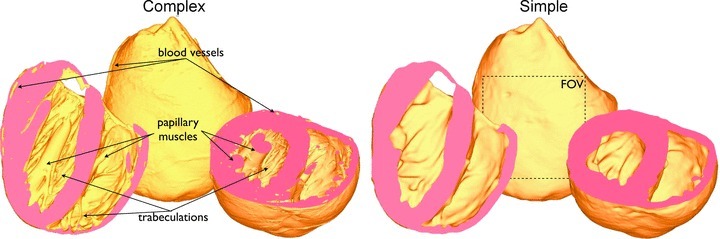
Complex model (left) containing fine-scale anatomical features such as blood vessels, papillary muscles and trabeculations, and simple model (right) with such fine-scale features removed. Also shown in simplified model is the square epicardial field-of-view (FOV) used to count wavefront numbers.

Simulating electrical activation

Electrical activation throughout the ventricular model was simulated using the bidomain equations (Henriquez, 1993), the implementations of which have been described previously (Vigmond et al. 2008). During certain protocols it was preferable to represent the cardiac tissue as a single conducting domain, whereby the bidomain equations are reduced to the monodomain equation and the harmonic mean conductivity tensor used to match bidomain conduction velocities (Bishop & Plank, 2010).

Cellular ionic dynamics, defining the total membrane current, were represented by a recent rabbit ventricular cell model (Mahajan et al. 2008b). Ionic model parameters were initially left at their default values for arrhythmia simulation which led to the induction of arrhythmias with tachycardia-like complexity. Such arrhythmias were characterised by visually less disorganisation in the spatio-temporal wavefront dynamics and will be referred to here as tachyarrhythmias.

In addition, action potential duration (APD) was decreased in the ventricular cell model through a slight modification of the parameter controlling the recovery from inactivation of the L-type calcium channel, which controls restitution and spiral-wave stability without significantly impacting action potential morphology (Mahajan et al. 2008a). The parameter, termed R(V) in the Mahajan et al. (2008) model, was multiplied by a factor of 5. Such a modification resulted in wavefronts which were characterised by visually higher disorganisation in their spatio-temporal dynamics than during tachyarrhythmias (for example a higher number of smaller, isolated wavefronts which broke up more frequently and showed less repeatable pathways), and will be referred to here as fibrillatory arrhythmias. Intra- and extracellular conductivities were based on those of Roberts & Scher (1982), adjusted to reduce conduction velocity in all directions by 25% to replicate the slowed conduction during heart failure (Akar et al. 2004, 2007; Tomaselli, 2004; Nattel et al. 2007; Stevenson & Sweeney, 2007), which in the rabbit has been attributed to down-regulation of connexin-43 (Ai & Pogwidz, 2004). Such a reduction in activation wavelength is also commonly used in experimental studies through either the use of pharmacological uncoupling agents (such as 2,3-butanedione monoxime (BDM); Lou et al. 2012) or the use of flecainide to slow conduction (Li et al. 2009) due to the widely reported difficulties in successfully sustaining reentrant activity in otherwise healthy rabbit ventricles (Manoach et al. 1980; Cheng et al. 2004; Lou et al. 2012). Such a reduction in CV thus not only allowed simulation of more clinically relevant arrhythmia behaviour during heart failure, but also allowed sustained arrhythmias to be induced, and facilitated comparison with previous experimental studies. Conductivity of the extracellular bath was 1.0 S m⁻¹ (isotropic).

The bidomain and monodomain equations above were solved with the finite element method within the Cardiac Arrhythmia Research Package (CARP) (Vigmond et al. 2003), the underlying numerical details of which have been described extensively elsewhere (Plank et al. 2007, 2009; Vigmond et al. 2008).

Simulation protocol

Episodes of arrhythmias were induced within both complex and simplified models using an S1–S2 stimulation protocol. Prior to arrhythmia induction, both models underwent a preconditioning phase constituting eight pacing stimuli applied to a site on the right ventricle (RV) free wall close to the apex (of strength 0.005 μA cm⁻³, duration 1 ms) at a basic cycle length of 240 ms to ensure steady-state. At a variable coupling interval (CI) following the final pacing stimulus (when the recovery isoline was approximately mid-way between apex and base) the S2 shock (of strength <2 V cm⁻¹, 5 ms duration) was applied via a plate-electrode set-up at the edges of the surrounding bath, as used previously (Bishop et al. 2010b, 2011). Post-shock activity was simulated for a total of 2500 ms for each episode. In all, 13 different episodes of arrhythmias were induced in both models through using CIs between 180 and 240 ms in 5 ms increments. A monodomain representation was used for preconditioning and post-shock simulation, with a full bidomain representation used for simulation of S2 shock delivery and the 5 ms of activity immediately following the shock. Simulation states were check-pointed and restarted to switch between monodomain and bidomain simulation environments, as used previously (Bishop et al. 2011).

Quantitative arrhythmia analysis

Arrhythmia durations

Total durations of arrhythmias were defined as the time from shock induction (shock-end) to that time at which all wavefront activity within the model was eliminated, i.e. all nodes having transmembrane voltage (V_m) levels <−80 mV. Only the first 1.5 s of activity was quantitatively analysed; the following 1 s was simulated only to obtain a more accurate measure of arrhythmia durations.

Filament analysis

Filaments are the organising centres of reentrant activity and can be thought of as the 3D analogue of the centre of spiral waves (phase singularities). The algorithm used for filament detection and the methods for identifying individual filaments in space and tracking their dynamics in time were based upon previous studies (Fenton & Karma, 1998; Clayton & Holden, 2002; ten Tusscher et al. 2007), adapted for use on unstructured finite element meshes used in this study, as detailed previously (Bishop et al. 2011). Throughout each simulation, all filament interactions (birth, death, division and amalgamation) were recorded along with total filament numbers and mean lengths at each time step. Total filament interaction rate was defined as the sum of the birth, death, division and amalgamation rates. The intersections of filaments with epicardial triangles within the model were identified and counted as unique surface phase singularities.

Wavefront analysis

Images of V_m distributions over the entire posterior epicardial surface were obtained at 1 ms intervals throughout the duration of the arrhythmias. The images, which had an intensity-based colour (grey) scale were then cropped to select only a square region (dimension 1 × 1 cm) representing the typical FOV in an optical mapping experiment, shown in Figure 1B. Intensities of voxels within the image were then translated from V_m to represent phase (θ), using the time-delay method (Clayton et al. 2006) with an optimised delay of 2 ms and a potential reference of −20 mV. A threshold of π/2 –π applied to the phase map selected only points undergoing depolarisation, thus delineating wavefronts within the image. Application of a connected component algorithm to the threshold image was then used to identify the number of individual, connected wavefronts present within each mapped epicardial window at each time step, thus denoting the number of epicardial surface wavefronts.

Electrocardiograms

Pseudo-electrocardiogram (ECG) traces were computed as bipolar extracellular electrograms by subtracting two unipolar electrograms, measured with an Einthoven configuration, approximated by a lead configuration used previously (Bishop & Plank, 2011). Dominant frequencies (DFs) were calculated directly from pseudo-ECG traces following preprocessing with a fast fourier transform. As used here, the DF measure represents the frequency of the largest amplitude peak in the pseudo-ECG signal spectrum.

Activation rate calculation

Activation rates were derived individually for each node in the mesh by calculating the number of full depolarisations of membrane potential occurring during each arrhythmia episode.

Statistical analysis

Throughout, unless otherwise specified, data are presented as means ± standard deviation. Student's t test for unpaired data was used to test statistical significance between quantitative arrhythmia dynamics of anatomically complex and simplified models. Throughout individual arrhythmia episodes, maximum numbers of filaments, surface phase singularities and wavefronts occurring at any one time frame (1 ms) were also recorded. Average maximum values over all 13 episodes were then calculated, in addition to the average mean numbers for each episode.

Results

Dynamics of simulated tachyarrhythmias

Post-shock activity was simulated following 13 different shock-induction episodes with CIs between 180 and 240 ms for both anatomically complex and simplified models. Cellular ionic dynamics within the rabbit ionic model (Mahajan et al. 2008b) were initially left unaltered at the default values. This allowed successfully induced episodes of arrhythmias to be obtained for all 13 cases, with characteristic visual complexity of that of tachyarrhythmias.

Qualitative analysis of wavefront dynamics

Figure 2 shows qualitative analysis of the evolution of simulated activation wavefronts over a 1000 ms period for an arrhythmia with CI = 210 ms in both the anatomically complex (top panel) and simplified (bottom panel) models. As can be seen from the figure, the fundamental patterns and dynamics of the arrhythmias are very similar between both models, in terms of the number of wavefronts present, and their respective activation wavelengths and trajectories. In each case, the arrhythmias appear to be driven by a large rotor on the posterior epicardial surface rotating in a clockwise direction and causing successive sweeping wavefronts to wrap around the RV free wall in the posterior–anterior direction. The septum is also seen to play an important role here, depending on the relative state of the arrhythmia and the respective refractoriness of the septum: either two wavefronts (originating from the anterior and posterior sides of the ventricles) propagate down the septum towards one another and collide (complex panel image 1000 ms, simple panel 400 ms image), or else unidirectional propagation occurs, with the septal wavefront breaking out onto the anterior/posterior walls in advance of the main propagating epicardial wavefront, causing collision and at times wavebreak upon interaction (see Supplemental Movies of arrhythmias). Importantly, as evidenced in both Figure 2 and the Supplemental Movies, the additional anatomical complexity of the complex model is not visually seen to significantly alter the model's behaviour during arrhythmias; no anchoring or pinning of reentrant cores is apparent. Although each arrhythmia episode was very different due to their inherent chaotic nature, corresponding similarities to those described above between complex and simplified models were seen through all episodes, each of which can be viewed as a movie in the Supplemental Material.

Figure 2. Wavefront dynamics during an arrhythmia episode (CI = 210 ms) in the anatomically complex (top) and simplified (bottom) models.

Posterior (upper) and anterior (lower) epicardial views are shown, with clipping planes exposing intramural and endocardial activation in an inclined posterior view (centre).

Quantitative analysis of global metrics

Overall, there was no significant difference in the duration of the sustained simulated arrhythmias between each model. The mean arrhythmia duration was 1248 ± 430 ms in the complex model, compared to 1288 ± 547 ms – all episodes self-terminated within <2500 ms. Furthermore, both models had the same numbers of short-lived (<750 ms, 3 each) and long-lived (>1750 ms, 3 each) arrhythmia episodes.

The bipolar pseudo-ECG recordings also appeared very similar between models, as demonstrated in Fig. 3, which plots the lead I pseudo-ECG trace for the complex (red) and simplified (blue) models over the duration of the arrhythmia episodes with CI = 185 ms. Although the complex model pseudo-ECG does appear to be slightly less smooth in places than the simplified model, overall the morphology of the traces are very similar indeed and produced similar DFs, both being 5.33 Hz. Such a similarity in DFs between models was also witnessed throughout all induced arrhythmia episodes with the mean DFs of lead I traces over all episodes being 4.84 ± 0.65 Hz for the complex model, compared to 5.06 ± 0.28 Hz for the simplified model.

Figure 3.

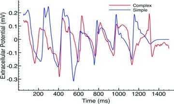
Bipolar pseudo-ECG recordings from lead I during arrhythmia episode with CI = 185 ms for complex (red) and simple (blue) models.

Quantitative analysis of 3D intramural metrics of complexity

Although qualitative analysis of the wavefront dynamics and global metrics revealed little differences between anatomically complex and simplified models, a detailed quantitative analysis of metrics relating to localised 3D intramural activity highlighted a number of distinct and important differences.

Filament numbers. Figure 4A, top, plots the variation in the total number of filaments over the duration of simulated arrhythmia episodes with CI = 185 ms in the complex (red line) and simple (blue line) models. Note, the complex model episode was sustained for >1500 ms, whereas the simple model episode terminated after approximately 1300 ms. Here, we can clearly see that the complex model episode consistently produces a larger number of individual filaments over the duration of the arrhythmia than the simplified model. The mean number of filaments at each time frame during which the arrhythmia was sustained was 5.95 (with a maximum at any one frame of 17) in the complex model, compared to 4.04 (max 10) in the simple model. This difference was even more noticeable when averaging over all 13 episodes, shown in the lower panel of Fig. 4A, with the complex model having an average number of filaments of 5.09 ± 1.15 (with an average number of maximum filaments occurring in any one frame over all episodes being 16.9 ± 2.00), compared to that of the simple model being 3.09 ± 0.70 (max 9.77 ± 1.83), a statistically significant difference for both mean and max (P < 0.0001).

Figure 4. Quantitative analysis of 3D complexity metrics.

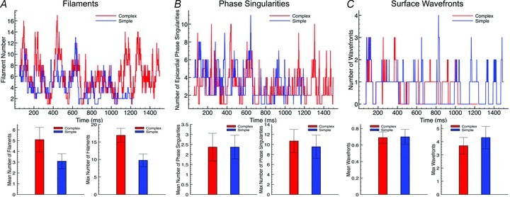
Top panels, total number of filaments for episode CI = 185 ms (A), epicardial surface phase singularities for episode CI = 185 ms (B), and surface wavefronts within selected FOV (shown in Fig. 1) for episode CI = 195 ms (C), plotted over entire arrhythmia duration for complex (red) and simple (blue) models. Bottom panels, mean (left) and max (right) numbers of above plotted quantities averaged over all 13 arrhythmia episodes.

As the anatomically complex model has a larger tissue volume (represented chiefly by the papillary muscles), we also quantified (for the complex model) the mean number of filaments over all episodes which had more than 50% of their total length within a papillary muscle: over all episodes the mean number of such papillary filaments was 0.26 (max 4.08). This thus suggests that, although they represent a contributing factor, the additional endocardial structures were not the main source of the additional filament numbers seen in the complex model.

Filament interactions. The large difference in filaments numbers between models seen above was also paralleled by statistically significant differences in other metrics which quantify filament dynamics and interactions. For example, over all 13 arrhythmia episodes, the complex model showed a significantly higher total interaction rate (1.11 ± 0.26 ms⁻¹) than the simple model (0.30 ± 0.05 ms⁻¹, P < 0.001), with a larger total filament production rate being 0.53 ± 0.13 ms⁻¹ compared to 0.14 ± 0.03 ms⁻¹ (P < 0.001), respectively. Consequently, the mean lifetimes of filaments was also significantly smaller in the complex model (9.11 ± 0.76 ms) compared to the simple model (20.0 ± 2.0 ms, P < 0.0001). However, importantly, the average maximum filament lifetime of any filament during each arrhythmia episode was similar between models, being 223 ± 76 ms and 254 ± 92 ms in the complex and simplified models, respectively.

Filament lengths. The mean length of all filaments existing within the models at each time frame, averaged over all episodes, was consistently significantly shorter in the complex (109.6 ± 17.8 elements) compared to the simple (151.9 ± 22.1) model (P < 0.001). However, the average maximum length of filament at each time frame over all episodes was similar in both models, being 244 ± 52 and 247 ± 38 elements in the complex and simplified models, respectively.

Quantitative analysis of 2D surface metrics of complexity

Although the above analysis of intramural filament dynamics appeared to suggest significant differences between the two models, this is at odds with the global analysis in the first section, which showed very close similarities in wavefront patterns and pseudo-ECG frequencies. To further investigate this, in Fig. 4B and C top panels we plot the variation in the number of total epicardial surface phase singularities and the number of individual wavefronts within an epicardial window over the duration of the simulated arrhythmia episodes with CI = 185 ms and CI = 195 ms, respectively, for the two models. The two plots show that both models maintain very similar numbers of surface phase singularities and wavefronts throughout the duration of the arrhythmias: the complex model had an average (over the arrhythmia duration) of 2.89 phase singularities (max 10) and 0.77 individual wavefronts (max 4), compared to 3.18 (max 11) and 0.52 (max 4), respectively in the simplified model. This similarity is further witnessed when observing the averages of these quantities over all 13 episodes, shown in the lower panels of Fig. 4B and C, suggesting that the underlying arrhythmia complexity is indeed similar in both models.

Correlation with anatomical structures

In order to investigate the potential interaction between anatomical structures and the individual wavefronts during simulated arrhythmias (which were not evident visually in Fig. 2 or the Supplemental Movies), Fig. 5 plots the spatial variation in mean activation rate (see the section Activation rate calculation), averaged over all 13 arrhythmia episodes, of each node point within the finite element models. Although minor differences are apparent between models, over all, both models produce similar spatial distributions of activation rates, with higher rates being concentrated in the basal left ventricle (LV), perhaps due to the higher tissue volume in this region, with the apical RV showing lower rates.

Figure 5. Spatial distribution of mean nodal activation rate (activations s⁻¹), averaged over all 13 arrhythmia episodes, within the entire volume of the ventricles.

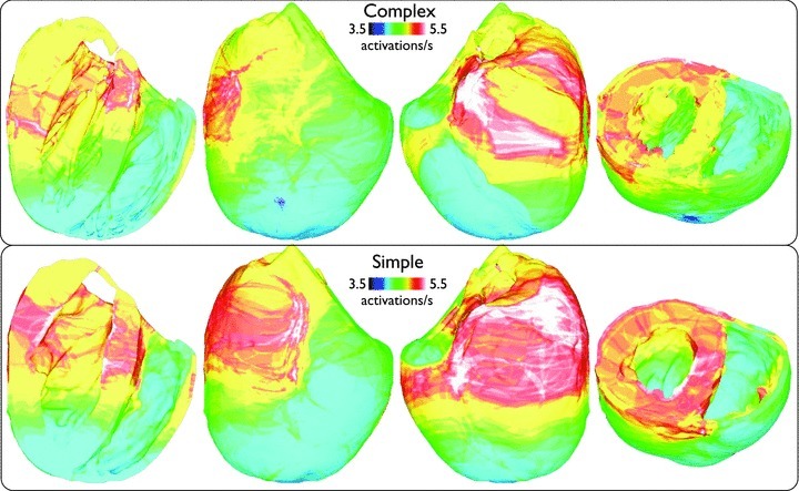
Plots are shown on anterior/posterior epicardial surfaces and posterior views where longitudinal/transverse clipping planes have been used to allow endocardial surfaces to be viewed.

To investigate how the filaments themselves interact with the model anatomy, Fig. 6 now plots the spatial distribution of all filament trajectories over the total duration of all simulated arrhythmia episodes. Here, the cumulative number of milliseconds in which a given element within the finite element model was associated with part of a filament is summed up for all 13 episodes and plotted, allowing localisation of filaments within particular regions throughout the volume of the ventricles to be assessed.

Figure 6. Spatial distribution of the cumulative temporal filament count, within the entire volume of the ventricles, accumulated over all 13 arrhythmia episodes for complex (top) and simple (bottom) models.

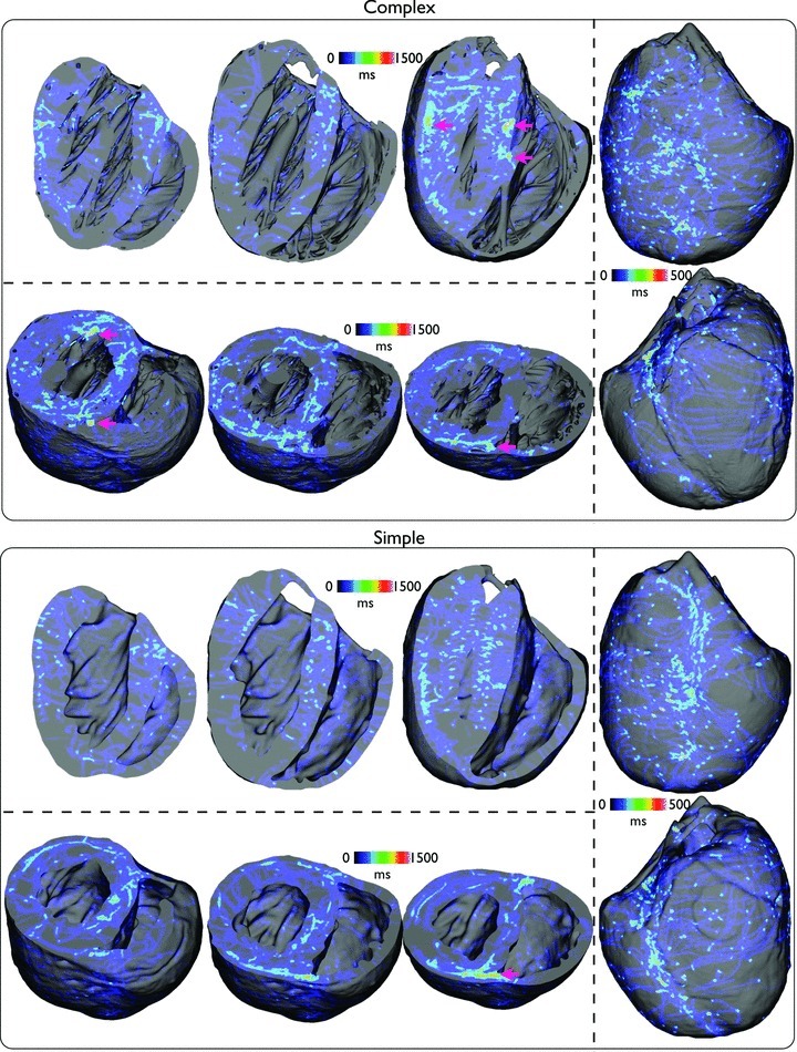
Plots are shown on anterior/posterior epicardial surfaces (right panel) and posterior views where longitudinal (top panel) and short-axis (bottom panel) clipping planes have been used to allow endocardial surfaces and intramural distributions to be viewed at different clipping locations through the ventricles.

Figure 6 shows that, in both models, the filaments take a variety of trajectories, although, in line with the findings in Fig. 5, much of the activity preferentially takes place in the LV. One important difference is the appearance of slight ‘hot spots’ of filament activity, highlighted by pink arrows in the figure, which are seen more frequently in the complex model, primarily close to the endocardial surface in the neighbourhood of papillary muscle and large trabeculae insertion sites. However, an additional occurrence of such a hot spot is also seen close to the septal junction with the posterior free-ventricular wall which is also present in the simplified model (visible in short-axis clipping-plane images).

Dynamics of simulated fibrillatory arrhythmias

Cellular ionic dynamics were then altered, as described in the section Simulating electrical activation, to induce more sustained spiral-wave break-up and arrhythmias with a more complex, VF-like visual appearance. Overall, this led to arrhythmias being sustained for significantly longer durations than in the case of tachyarrhythmias.

Qualitative analysis of wavefront dynamics

Figure 7 analyses the activation wavefront dynamics of the simulated arrhythmias with CI = 225 ms over 1300 ms duration in both models. Firstly, in both models, the wavefront patterns during fibrillatory activity shown in Fig. 7 appear qualitatively more disorganised than those in Fig. 2 for tachyarrhythmia activity. Many more individual wavefronts are seen to exist throughout the volume of the ventricles, which have a higher instance of wavebreak and move with shorter wavelengths in less repeatable trajectories. Despite this increased complexity, though, as is particularly evident by the Supplemental Movies, a degree of periodicity and organisation still exists in the wavefront patterns.

Figure 7. Wavefront dynamics in the complex (top) and simplified (bottom) models during an arrhythmia episode (CI = 225 ms) with fibrillatory dynamics.

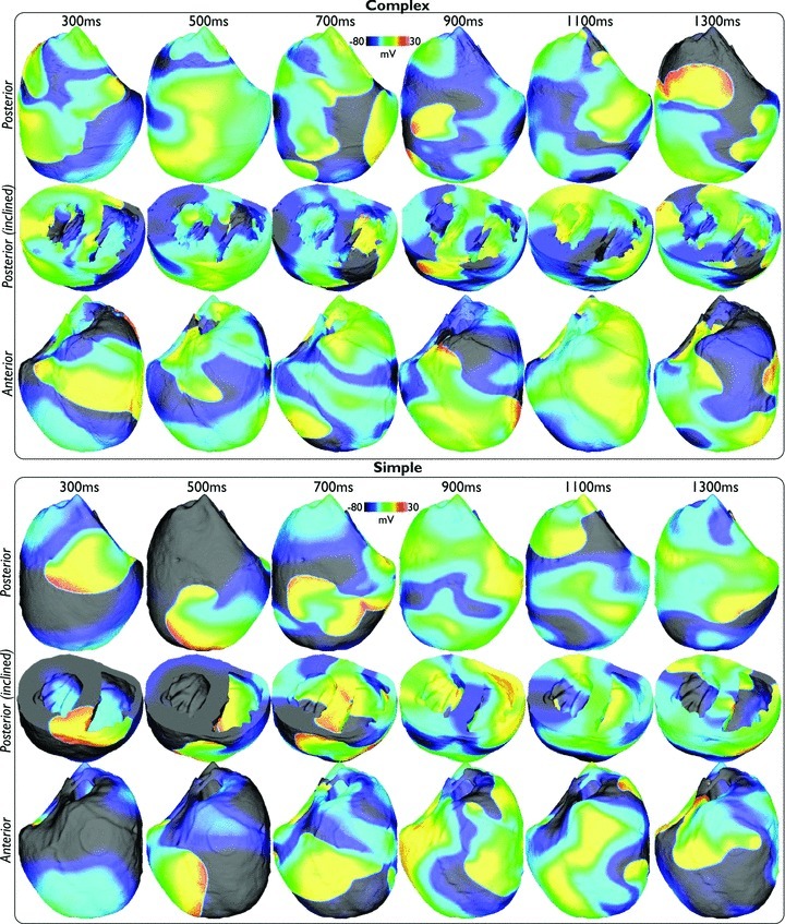
Posterior (upper) and anterior (lower) epicardial views, with intramural and endocardial activation exposed in an inclined posterior view (centre).

During tachyarrhythmia activity the wavefront dynamics in Fig. 2 appeared visually very similar between complex and simplified models. However, during fibrillatory activity there appears subtle differences between the wavefront dynamics shown in the snap-shots of Fig. 7 between models, specifically the number of individual wavefronts and the instances of wavebreak appearing marginally higher in the complex model. Again, this trend for this episode pair, as well as others, is also visible in Supplemental Movies.

Quantitative analysis of global metrics

Overall, the simulated arrhythmias within the complex model were sustained for slightly longer durations than in the simplified model; eight episodes were fully sustained (did not self-terminate within the full 2500 ms simulation time) in the complex model, compared to five in the simplified case, whilst the simplified model had a larger number (seven) of short-lived episodes <750 ms, compared to three in the complex model case. As a result of many episodes in both models being fully sustained, calculating mean arrhythmia durations was not possible.

However, as during tachyarrhythmias, the bipolar pseudo-ECG recordings appeared very similar between models, as demonstrated in Fig. 8, which plots the lead II pseudo-ECG traces over the duration of the arrhythmia episodes with CI = 200 ms. Although, in places the complex model pseudo-ECG does again appear slightly less smooth than the simple model pseudo-ECG, the two traces have similar DFs, being 8.67 Hz and 7.33 Hz. For all 13 arrhythmia episodes, mean DFs were also similar between models, being 6.36 ± 2.11 Hz and 6.05 ± 2.24 Hz, respectively.

Figure 8.

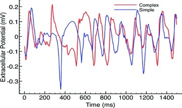
Bipolar pseudo-ECG recordings from lead II during arrhythmia episode with CI = 200 ms for complex (red) and simple (blue) models.

Quantitative analysis of 3D intramural metrics of complexity

Here, as in the section Quantitative analysis of 3D intramural metrics of complexity, we now conducted a detailed quantitative analysis of metrics relating to localised 3D intramural activity to further investigate differences in arrhythmia dynamics between models.

Filament numbers. Figure 9A shows how the total number of filaments varies over the duration of arrhythmia episodes with CI = 225 ms in the complex (red line) and simple (blue line) models. As in the case of the tachyarrhythmias in Fig. 4A, the complex model episode consistently produces a larger number of individual filaments, although this appears now to be further amplified in this fibrillatory state. Such a significant trend was witnessed throughout all 13 episodes, with the mean filament number per episode being 9.96 ± 2.60 (max 26.40 ± 5.42) in the complex model, compared to 4.85 ± 2.95 (max 12.15 ± 6.73) in the simplified model (P < 0.0001). As before, the mean number of filaments per episode that had 50% or more of their length within a papillary muscle was also quantified, here found to be 0.49 (max 4.62), again demonstrating that the increased number of filaments in the complex model was not due to the increased tissue volume represented by the papillaries.

Figure 9. Quantitative analysis of 3D complexity metrics during fibrillatory activity.

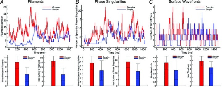
Top panels, total number of filaments for episode CI = 225 ms (A), epicardial surface phase singularities for episode CI = 220 ms (B), and surface wavefronts within selected FOV (shown in Fig. 1) for episode CI = 225 ms (C) plotted over entire arrhythmia duration for complex (red) and simple (blue) models. Bottom panels, mean (left) and max (right) numbers of above plotted quantities averaged over all 13 arrhythmia episodes.

Filament interactions. The significant difference in filaments numbers between models seen above was again also witnessed in large differences in other filament dynamics metrics, with the complex model showing significantly higher total interaction rates (1.65 ± 0.39 ms⁻¹ versus 0.31 ± 0.19 ms⁻¹, P < 0.0001), higher filament production rates (0.79 ± 0.19 ms⁻¹ versus 0.14 ± 0.09 ms⁻¹, P < 0.0001), and shorter filament lifetimes (11.94 ± 0.63 ms versus 28.20 ± 7.57 ms, P < 0.0001). However, as was found during the tachyarrhythmia episodes, the average maximum filament lifetime of any filament during each arrhythmia episode was similar, being 303 ± 75 ms and 278 ± 152 ms in the complex and simplified models, respectively.

Filament lengths. As in the case of tachyarrhythmias, the complex model is again seen to produce filaments with a significantly smaller mean length than the simple model. Over all episodes, however, this difference is even greater than for tachyarrhythmias with the complex model filaments having less than half the mean length of those of the simple model (95.3 ± 14.8 versus 202.2 ± 59.1, P < 0.0001) and a smaller average maximum filament length (255.6 ± 45.3 versus 355.6 ± 69.4, P < 0.0005).

Quantitative analysis of 2D surface metrics of complexity

Analysis of epicardial wavefront and phase singularity numbers during simulated tachyarrhythmias above revealed close similarities between the two models, despite significant differences in intramural filament numbers and dynamics. In the case of fibrillatory activity, however, Fig. 9B and C, which plot the number of epicardial phase singularities and wavefronts during arrhythmia episodes with CI = 220 ms and CI = 225 ms, respectively, shows the arrhythmia dynamics of the epicardial surface appearing slightly more disorganised in the complex model, with more phase singularities and wavefronts over the duration of the arrhythmia than the simplified model. This trend is emphasised in the lower panels of Fig. 9B and C, which show that over all 13 episodes the complex model appears to produce arrhythmias with significantly higher numbers of epicardial phase singularities (mean 5.65 ± 1.66, average maximum number at any one time 18.54 ± 4.40) and epicardial surface wavefronts (mean 1.14 ± 0.32, average maximum number at any one time 5.85 ± 1.14) compared to the simple model (phase singularities: 3.79 ± 2.95 (P < 0.05), max 11.23 ± 5.86 (P < 0.002); epicardial wavefronts 0.77 ± 0.45 (P < 0.05), max 4.31 ± 1.44 (P < 0.01)). Note, though, that the higher P values here indicate less strong statistical significance than elsewhere in the study. In addition, due to the fact that a large number of arrhythmia episodes in the simplified model (7) were sustained for <750 ms, the above analysis was repeated, this time excluding such short-lived episodes in both models. Although the complex model still showed a larger number of phase singularities (5.95 ± 1.72 versus 5.41 ± 2.68) and surface wavefronts (1.24 ± 0.28 versus 1.04 ± 0.50) than the simplified model, this difference was no longer statistically significant at the 5% level.

Correlation with anatomical structures

Figure 10 plots the spatial variation in mean activation rate (averaged over all 13 arrhythmia episodes) at each node within the finite element models. Here, we can see that both models again show similar activation rate maps, as witnessed previously during tachyarrhythmias. However, importantly here, such a close match was only obtained through using a colour-bar scale with slightly higher limits in the complex model (5.5 − 8 s⁻¹) to those used in the simple model (4 − 7 s⁻¹), indicating an overall marginal increase in activation rate of all regions of the ventricles in the anatomically complex model.

Figure 10.

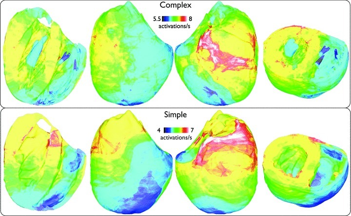
Spatial distribution of mean nodal activation rate (activations s⁻¹), averaged over all 13 arrhythmia episodes, within the entire volume of the ventricles for fibrillatory activity with similar viewing angles to Fig. 5.

Figure 11 now plots the spatial distribution of all filament trajectories over the total duration of all arrhythmia episodes. Note that in this case, due to the fact that the arrhythmias of the simple models were typically sustained for shorter durations than the complex model episodes, the time scales on the colour bars have also been adjusted between the two models. Firstly, we notice the existence of far more filament trajectories, particularly on the epicardium in both models, relative to the case of tachyarrhythmias. Similarly to Fig. 6, however, the complex model shows the existence of a larger number of ‘hot-spots’ where the filaments have spent a relatively large amount of time, clustered primarily close to endocardial insertion sites of papillary muscles and larger trabeculations (highlighted by pink arrows). Comparing directly with the analogous plot of Fig. 6, however, these clustering hot-spots appear to be slightly more numerous and brighter than during tachyarrhythmias. However, we note again that, despite the existence of these slight ‘hot-spots’, no such anchoring of rotors was visibly identifiable in the arrhythmia movies in Supplemental Material. Furthermore, here we additionally see a large amount of filament clustering on the posterior epicardial surface close to the apex of the complex model near to where the septum joins the free wall. Finally, a similar clustering is seen intramurally, close to the intersection of the septum with the posterior wall witnessed in both models, as in the case of tachyarrhythmias.

Figure 11.

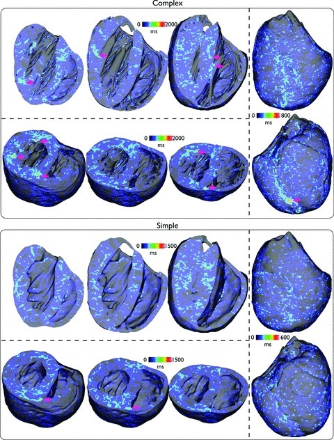
Spatial distribution of the cumulative temporal filament count, within the entire volume of the ventricles, accumulated over all 13 arrhythmia episodes for complex (top) and simple (bottom) models during fibrillatory activity with similar viewing angles as used in Fig. 6.

Comparison and validation with experimental data

Finally, in this section we bring together the simulated results presented above and provide a detailed comparison with previously reported experimental measurements of arrhythmia dynamics in the rabbit ventricles in order to validate the findings presented. All studies are optical mapping recordings from Langenndorff-perfused rabbit hearts.

Shock-induction of arrhythmias

The CIs (180–240 ms) used in this study to successfully induce arrhythmias within the computational models fall within the vulnerable window of 80–140% APD reported in a very recent experimental study by Lou et al. 2012 (for APD < 170 ms) in addition to other earlier experimental shock-induced arrhythmogenesis investigations which successfully induced arrhythmias with CIs of 130–230 ms (Banville et al. 1999). A further means of experimental validation of our results is also shown in the study by Lou et al., who report the difficulty in sustaining ventricular arrhythmias in the young healthy rabbit heart without the use of pharmacological interventions, as has also been stated elsewhere in the literature (Manoach et al. 1980). Less than 30% of shocks induced any form of arrhythmia, and of those <2% were sustained for more than six beats. The inclusion of the electromechanical uncoupling agent BDM (which the authors show produces an approximate 25% shortening of activation wavelength) increased the inducability and sustainability of the arrhythmias with 30% of induced arrhythmias sustained for more than six beats with BDM (a previous study by the same group showed 37%; Cheng et al. 2004). These figures closely match our findings: following a 25% reduction in activation wavelength (brought about through reducing CV), we found that 4/13 (30.8%) and 6/13 (46.1%) in complex/simple models were sustained for more than six beats during tachyarrhythmias. Similar to the experimental findings (Lou et al. 2012), without such a reduction in CV/activation wavelength, no arrhythmias could be sustained for more than six beats.

Dynamics of tachyarrhythmias

Little experimental data can be found detailing the dynamics of tachyarrhythmias without the use of any form of pharmacological agent due to the above noted difficulties in sustenance. The study by Cheng et al. (2004) showed that, when BDM is used the number of phase singularities recorded from the anterior epicardial surface was 1.5 ± 0.5 during sustained episodes of ventricular tachycardia (VT); extrapolating to the entire epicardial surface suggests approximately three phase singularities were present in total. An earlier study by Gray et al. (1995) using the uncoupler diacetyl monoxime (DAM) concluded that one to two surface rotors in total were thought to sustain VT in the rabbit ventricles. Our findings compare favourably with these experimental results as we showed 2.37 ± 0.62/2.37 ± 0.59 epicardial phase singularities occurred during tachyarrhythmia episodes in complex/simple models.

Dynamics of fibrillatory arrhythmias

As is the case with tachyarrhythmias, little experimental data exists on the dynamics of VF in healthy rabbit hearts, and for those studies which do exist, experimental recordings are limited at measuring only surface activity and thus cannot track or analyse full 3D filament information, which is the main metric used in this study to quantify complexity. Nonetheless, below we have drawn close comparison with the available data.

Phase singularity numbers. Chen et al. 2000 recorded the dynamics of VF in healthy rabbit hearts without the use of any pharmacological uncoupling agent (although it is not clear how this was achieved given the failure of such attempts without pharmacological intervention from other accomplished experimentalists). Interpretation of their results suggests a total of approximately 1.8 surface phase singularities were recorded within their mapping window (stated to be <40% of the total epicardium), giving a total of approximately 4.5 phase singularities over the total epicardial surface. A later study by Liu et al. 2003 using the uncoupler Cyto-D reported slightly higher phase singularity counts, seeming to centre around 5 phase singularities within the mapped window (suggesting <10 over the total epicardium), whilst another study using Cyto-D by Hayashi et al. 2007 reported phase singularity counts of close to 1 during short VF (<10 s) and close to 3 during long VF (>1 min), suggesting total epicardial counts in the region of 2–6. In all, the phase singularity counts found in our study during fibrillatory activity of 5.65 ± 1.66 and 3.79 ± 2.42 in complex/simplified models, respectively, lie within these experimental ranges. However, we also note that if we restrict our analysis to only those episodes of VF which were fully sustained (>2.5 s), the mean number of phase singularities found in the two respective models were slightly higher at 6.53 ± 1.04/6.58 ± 1.14 demonstrating a similar increase in VF complexity with duration seen in Hayashi et al. (2007). Finally, the computational modelling study by Clayton (2008) simulated VF dynamics in a histologically derived rabbit ventricular model, and reported a mean number of 6.3 filaments, which is within the range of mean filament numbers reported here in the complex/simplified models. This result demonstrates the similarity in simulated VF dynamics between histologically and MR-derived rabbit ventricular models.

Rotor lifetimes. The study by Chen et al. (2000) also recorded the lifetimes of surface phase singularities, reporting the mean phase singularity lifetime to be 14.7 ms with 51% lasting <8 ms and 98% lasting <1 rotation. Although we did not explicitly record phase singularity lifetimes here, the lifetimes of filaments within the simplified model (without intramural structures to alter the dynamics) will be closely correlated to phase singularity lifetimes: we find 54.3% of filaments were sustained <8 ms with 97.4% lasting less than 1 rotation, which shows a very close agreement with the experimental results of Chen et al. (2000).

DF of pseudo-ECGs. The mean DFs during fibrillatory activity in both models are slightly lower than those reported experimentally where 11.5 ± 3.5 Hz has been considered average (Panfilov, 2006) and 12.6 ± 4.0 was reported in Chen et al. (2000). However, other studies have reported much lower DFs in the rabbit of <8 Hz (Gray et al. 1998). The lower values in our study could be partially explained by the reduced CV used in our study, reducing activation rate, relative to Chen et al. (2000), for example. Furthermore, the electrodes used to record the pseudo-ECGs in our set-up were positioned a few millimetres from the epicardial surface, which would act to smooth out the recorded spatial distribution of extracellular potential. This could then be expected to cause a shift in the spectrum to lower frequencies relative to the situation where signals are recorded directly from the epicardial surface as more common experimentally. Finally, in contrast to many experimental reports, we included in our analysis episodes which were not fully sustained which could have acted to lower the mean DFs in both models; we did not have the luxury to induce numerous episodes until a statistically significant number were fully sustained due to the huge computational burden required by each simulation run (as discussed below). For example, in those episodes of fibrillatory activity which were fully sustained, DFs (obtained from the full 2.5 s of activity) of 8–10 Hz were common (in 6/13 fully sustained episodes were in this range), which are within the experimental range above.

Discussion

Our results suggest that the overall dynamics of simulated tachyarrhythmias are very similar in both an anatomically complex computational rabbit ventricular model (containing fine-scale representations of endocardial structures and blood vessels) and in a simplified model lacking such features, as quantified by induced arrhythmia durations, epicardial wavefront/phase singularity counts, pseudo-ECG DFs, local tissue activation rates and importantly visual inspection of surface/intramural wavefront dynamics. During simulated fibrillatory arrhythmias, as activation wavelength was shortened reducing reentrant rotor core size, small differences in such arrhythmia dynamic metrics which quantified arrhythmia maintenance became apparent between models, with the anatomically complex model appearing to exhibit marginally more sustained, complex dynamics. Such conclusions regarding similarities or small differences in arrhythmia dynamics between models, however, are taken in the context of the apparent significantly larger numbers of filaments (and their interaction statistics) witnessed in the complex model, during both tachy- and fibrillatory arrhythmias. We attribute these differences to the interactions of filaments with intramural structures in the complex model. However, due to the closeness of other arrhythmia metrics between models, this does not appear to significantly affect overall dynamics and maintenance. Finally, although in both cases there was some evidence of filament clustering around papillary muscles and trabeculae ridges on the endocardium in the complex model (more so during fibrillation), this was not at all visually apparent in our simulations and much less so than has been witnessed in previous experimental studies performed mainly on larger animal models (Pertsov et al. 1993; Kim et al. 1999; Valderrabano et al. 2003).

Insight into reentrant arrhythmia dynamics in rabbit and other species

Recent computational modelling (Panfilov, 2006; Clayton, 2008; ten Tusscher et al. 2009) and experimental optical mapping (Jalife & Gray, 1996; Chen et al. 2000) findings have shown that VF is characterised by a smaller number of reentrant sources in the rabbit heart, showing strong periodicity, relative to the more complex excitation patterns seen in larger animal hearts such as the pig or dog (Valderrabano et al. 2003; Huang et al. 2005; ten Tusscher et al. 2009). Our study closely agrees with these findings, demonstrating that even when cellular ionic dynamics were altered during fibrillatory activity, full 3D analysis of wavefronts and filaments within the volume of the ventricles showed the mean number of reentrant sources driving the arrhythmic activity is still limited at approximately less than 10. We believe that the long total arrhythmia times simulated here, in terms of both the number of different episodes and their duration (2.5 s), further adds significant weight behind these particular findings. Furthermore, despite its apparent complexity, many of the episodes during fibrillatory-like arrhythmias were still seen to show strong elements of organisation, with large wavefronts propagating around repeatable pathways, not witnessed before.

Overall, during simulated tachyarrhythmias, the anatomically complex and simplified models showed remarkably similar arrhythmia dynamics, in terms of both their visual appearance of wavefronts and the quantitative analysis of filament behaviour. In simulations of fibrillatory activity, small differences became noticeable, but still many qualitative and quantitative features which measured arrhythmia maintenance remained similar. Although Figs 6 and 11 did appear to show a small degree of filament clustering around endocardial structures such as papillary muscles and trabeculations in the complex model (which was increased slightly during fibrillatory activity), there was little qualitative visual evidence of anchoring or pinning of reentry around such structures both from the still images of Figs 2 and 7 and the Supplemental Movies. The overall bi-ventricular geometry of the ventricles seemed to play the most important role in providing reentrant pathways for activation to support reentry. Our simulation results appear to suggest, therefore, that fine-scale anatomical structures may not provide such an important means of stabilising of rotors during arrhythmias in the rabbit heart, as has been reported in previous experimental mapping recordings of swine (Kim et al. 1999; Valderrabano et al. 2001, 2003; Nielsen et al. 2009) and dog (Pertsov et al. 1993) preparations. However, our results are in-line with the vast majority of previous experimental recordings from rabbit preparations (Jalife & Gray, 1996; Gray et al. 1998; Chen et al. 2000; Wu et al. 2002), which also did not report any apparent anchoring of rotors to anatomical structures. In a very recent study by Lou et al. (2012), however, a degree of anchoring was seen at the insertion site of the RV and septum, as also witnessed to an extent in our simulations (Figs 6 and 11), although no anchoring to other structures (papillary insertions, vessels, etc.) was reported. Of particular interest are the studies by Pak et al. (2003) and Wu et al. (2004) which demonstrate that VF can show anchoring to the papillary muscle insertion site in rabbit ventricles, but only under conditions of reduced excitability. Such a slowing of conduction would correspondingly reduce activation wavelength, similar to that achieved in our study through altering the cellular ionic dynamics to reduce APD, which saw a corresponding slight increase in anchoring (Fig. 11).

We suggest that the differing evidence for anchoring of rotors during reentrant arrhythmias to assist their sustainment is explained by considering the relative dimension of the rotor itself compared with that of the anatomical obstacle around which it may anchor; the smaller the reentrant rotor source relative to the size of the anatomical structure (papillary muscles, vessels, etc.), the more likely the structure is to act as a stabilising anchor. For example, in the case of larger animal hearts (pigs and dogs), the rotor size is small (they can sustain high numbers of reentrant sources within their volume; Panfilov, 2006; ten Tusscher et al. 2009) and the anatomical structure large, and thus anchoring occurs frequently, as reported (Pertsov et al. 1993; Kim et al. 1999; Valderrabano et al. 2001, 2003; Nielsen et al. 2009). Rabbit hearts, however, can contain fewer reentrant sources (Clayton, 2008; ten Tusscher et al. 2009), and thus the rotors are relatively large compared to the (relatively physically smaller) anatomical structures. However, when activation wavelength is reduced (through changes in conduction as shown experimentally (Wu et al. 2002; Pak et al. 2003), or APD as shown here), the rotor dimension is reduced, reducing the relative size of the rotor to the obstacle, and anchoring becomes more likely. Finally, it is also interesting to note that such reductions in excitability (which correspondingly reduce rotor size) can also be the result of pathological changes (Wu et al. 1998), in which case anchoring may be thought to play an increasingly important role in the rabbit ventricles.

Validation with previous experimental studies

We have demonstrated in the section Comparison and validation with experimental data that the fundamental arrhythmia induction protocols and dynamical behaviour during the induced simulated arrhythmias match closely to previous experimental reports during both ventricular tachy- and fibrillatory arrhythmias. Given that our computational model(s) was also constructed directly from high-resolution (25 μm resolution) MR data (Bishop et al. 2010b) and a highly biophysically detailed experimentally derived rabbit ventricular myocyte model of cellular dynamics (Mahajan et al. 2008b) was embedded within it, we can have a degree of confidence in the conclusions drawn from this study regarding the dynamics of arrhythmia maintenance in the rabbit ventricles and their relation to anatomical features. However, it is important to note that arrhythmia dynamics are known to vary with specific pharmacological interventions, an interesting issue which we suggest as an avenue of future study.

Utility of anatomically detailed models for studying reentrant dynamics

Throughout the analysis of both the simulated tachy- and fibrillatory arrhythmias, one anomaly existed in the quantification of filaments between the two models. Even during tachyarrhythmias, where no significant differences were witnessed in almost all other metrics, the complex model consistently gave significantly higher number of filaments, with shorter lengths and higher interaction rates. Importantly, however, in both arrhythmia cases the maximum filament lifetimes were similar in both models. We believe that the existence of intramural ‘holes’ represented by vessels and extracellular cleft spaces within the anatomically complex model may have caused filaments to temporarily ‘break-up’ as they pass over these discontinuities, causing the filament detection algorithm to record higher numbers of shorter filaments which interact more frequently.

However, this did not appear to affect the overall complexity of the arrhythmia, as defined by all other metrics similar in both models, which appears to be governed more by overall bi-ventricular geometry/size and activation wavelength. We thus suggest a level of caution in the sole use and interpretation of filament detection algorithms in similar models with high levels of intramural complexity in future studies.

An important consequence of the suggestion from our simulations that fine-scale anatomical details generally may not play a significant role in the maintenance of arrhythmias in the healthy rabbit heart is in relation to the necessary level of detail required in experimental imaging and model generation endeavours used for mechanistic enquiry regarding arrhythmia maintenance. For arrhythmia investigations in the rabbit, our conclusions suggest that the main requirement of imaging modalities used for model generation is that they faithfully resolve the overall bi-ventricular geometry. Finer-scale, more detailed structures appear to be of lesser importance to resolve in images and incorporate in subsequent models. This knowledge may then, in turn, guide the resolution of imaging data required from experimentalists, minimising both imaging time and equipment requirements, in addition to post-processing model generation and computational simulation demands (Plank et al. 2009). This is particularly important in the analysis of cardiac arrhythmias as the need to perform simulations of significantly long durations means that any increase in computational load from more detailed models must be justified.

Implications for future clinical modelling investigations

Despite known similarities in electrophysiological ‘effective size’ (which quantifies the ratio of electrical activation wavelength to physical ventricle size; Panfilov, 2006) between the rabbit and human, significant inter-species differences, particularly at the single cell level in action potential morphology, still exist. Consequently, the findings from this particular study cannot be directly extrapolated to shed light on human arrhythmia mechanisms. However, our study does describe a detailed computational modelling approach which could, in future investigations, be applied to high resolution human data to probe a similar question in clinical arrhythmia mechanisms. Specifically, a similar approach could be used to assess whether the relatively lower resolution standard clinical imaging data-sets (MR, CT), which on-the-whole cannot fully resolve fine-scale endocardial and intramural features, are adequate for model generation geared towards human arrhythmia investigations (Niederer et al. 2011a,b). This is a very important question, as maintaining fine-scale heterogeneities would be in keeping with the ‘personalisation’ of models and importantly will remove the simplification problem (i.e. where to define the ‘endocardial surface’) which can introduce significant bias. On the other hand, keeping such a high level of detail would also require higher-resolution imaging than is currently available in current standard clinical settings as well as significantly increase computational demands associated with model construction and simulation, meaning that using such detailed models within a clinical work-flow would be significantly more challenging.

Study limitations

Despite the use of HPC facilities and leading cardiac electrophysiology simulation environments, the simulations of arrhythmia episodes in this study represented an immense computational challenge. Although 2.5 s of activity took approximately 10 h to compute on 32 cores, the most significant challenge was the analysis, storage and curation of the resulting data files each of which occupied up to 50 Gb of storage. We were therefore not able to fully explore all of the parameter space relating to parameters which may alter the complexity and dynamics of the simulated arrhythmias, but instead chose just two sets which were used to produce tachy- and fibrillatory arrhythmias. In addition, the method of shock induction of arrhythmias was limited to the S1S2 protocol described in the Methods and thus, again due to computational considerations, it was not feasible to explore a variety of different arrhythmia initiation protocols. This may have been of more importance during tachyarrhythmias, as during fibrillatory arrhythmias the activity rapidly became less organised and so the means of initiation might play less of a role.

Although the anatomically complex model does represent an unprecedented amount of fine-scale structural detail (Bishop et al. 2010b), it does not currently represent electrophysiological heterogeneities, electromechanical coupling, histologically based microscopic structure or the Phase singularity, which may indeed impact the dynamics of the simulated arrhythmias. Recent simulation studies which incorporated the Phase singularity suggested that the Phase singularity does play an important role in prolonged post-shock VT, but is of lesser importance in shock-induced arrhythmogenesis and during the early phases of VT (Deo et al. 2009). In addition, we have only assigned myocardial cell types to the tissue represented within the model. In certain structures, for example some endocardial structures, the existence of non-myocytes could impact conduction in these regions; future investigation could therefore involve fully characterising these non-myocyte distributions throughout the ventricles and assessing their impact on electrical dynamics in light of the findings presented here. Furthermore, although the myocardial fibre orientation has been assigned within the model using a rule-based method based upon histologically and DTMRI-derived knowledge of fibre structure (Bishop et al. 2010b), its microscopic representation of fibre architecture around blood vessels (Bishop et al. 2010a) may not be entirely faithful, which could explain the complete lack of anchoring around vessels seen here. However, a recent study showed that the presence of fibre negotiation around vessels in fact attenuates conduction slowing around the obstacle (Gibb et al. 2009), suggesting anchoring would be less likely with smooth fibre negotiation. Although a specific feature of the rule-based approach for fibre direction assignment was the representation of an abrupt change in fibre angle at the insertion site of papillary muscles, it is possible that this change was too heavily smoothed by the algorithm, meaning conduction slowing in this region of our model is less pronounced and anchoring of filaments is not as likely as perhaps expected.

Glossary

APD

action potential duration

CI

coupling interval

DF

dominant frequency

ECG

electrocardiogram

FOV

field-of-view

HPC

high performance computing

LV

left ventricle

PS

Purkinje system

RV

right ventricle

VF

ventricular fibrillation

VT

ventricular tachycardia

Author contributions

M.J.B. and G.P. both made significant contributions to (1) the conception and design of experiments, (2) the collection, analysis and interpretation of data, and (3) the drafting of the article and revising it for important intellectual content.

Supplemental Data

Supplemental Movies

References

- Ai X, Pogwidz SM. Connexin 43 downregulation and dephosphorylation in nonischemic heart failure is associated with enhanced colocalized protein phosphatase type 2a. Circ Res. 2004;96:54–63. doi: 10.1161/01.RES.0000152325.07495.5a. [DOI] [PubMed] [Google Scholar]
- Akar F, Nass R, Hahn S, Cingolani E, Shah M, Hesketh G, Disilvestre D, Tunin R, Kass D, Tomaselli G. Dynamic changes in conduction velocity and gap junction properties during development of pacing-induced heart failure. Am J Physiol Heart Circ Physiol. 2007;293:H1223–H1230. doi: 10.1152/ajpheart.00079.2007. [DOI] [PubMed] [Google Scholar]
- Akar F, Spragg D, Tunin R, Kass D, Tomaselli G. Mechanisms underlying conduction slowing and arrhythmogenesis in nonischemic dilated cardiomyopathy. Circ Res. 2004;95:717–725. doi: 10.1161/01.RES.0000144125.61927.1c. [DOI] [PubMed] [Google Scholar]
- Banville I, Gray RA, Ideker RE, Smith WM. Shock-induced figure-of-eight reentry in the isolated rabbit heart. Circ Res. 1999;85:742–752. doi: 10.1161/01.res.85.8.742. [DOI] [PubMed] [Google Scholar]
- Beaumont J, Davidenko N, Davidenko JM, Jalife J. Spiral waves in two-dimensional models of ventricular muscle: formation of a stationary core. Biophys J. 1998;75:1–14. doi: 10.1016/S0006-3495(98)77490-9. [DOI] [PMC free article] [PubMed] [Google Scholar]
- Bishop MJ, Boyle P, Plank G, Welsch D, Vigmond E. Modeling the role of the coronary vasculature during external field stimulation. IEEE Trans Biomed Eng. 2010a;57:2335–2345. doi: 10.1109/TBME.2010.2051227. [DOI] [PMC free article] [PubMed] [Google Scholar]
- Bishop MJ, Plank G. Representing cardiac bidomain bath-loading effects by an augmented monodomain approach: application to complex ventricular models. IEEE Trans Biomed Eng. 2010;58:1066–1075. doi: 10.1109/TBME.2010.2096425. [DOI] [PMC free article] [PubMed] [Google Scholar]
- Bishop MJ, Plank G. Bidomain ECG simulations using an augmented monodomain model for the cardiac source. IEEE Trans Biomed Imag. 2011;58:2297–2307. doi: 10.1109/TBME.2011.2148718. [DOI] [PMC free article] [PubMed] [Google Scholar]
- Bishop MJ, Vigmond EJ, Plank G. Cardiac bidomain bath-loading effects during arrhythmias: Interaction with anatomical heterogeneity. Biophys J. 2011;101:2871–2881. doi: 10.1016/j.bpj.2011.10.052. [DOI] [PMC free article] [PubMed] [Google Scholar]
- Bishop MJ, Plank G, Burton R, Schneider J, Gavaghan D, Grau V, Kohl P. Development of an anatomically-detailed MRI-derived rabbit ventricular model and assessment of its impact on simulation of electrophysiological function. Am J Physiol Heart Circ Physiol. 2010b;298:H699–H718. doi: 10.1152/ajpheart.00606.2009. [DOI] [PMC free article] [PubMed] [Google Scholar]
- Chen J, Mandapati R, Berenfeld O, Skanes AC, Jalife J. High-frequency periodic sources underlie ventricular fibrillation in the isolated rabbit heart. Circ Res. 2000;86:86–93. doi: 10.1161/01.res.86.1.86. [DOI] [PubMed] [Google Scholar]
- Cheng Y, Li L, Nikolski V, Wallick DW, Efimov IR. Shock-induced arrhythmogenesis is enhanced by 2,3-butanedione monoxime compared with cytochalasin D. Am J Physiol Heart Circ Physiol. 2004;286:H310–H318. doi: 10.1152/ajpheart.00092.2003. [DOI] [PubMed] [Google Scholar]
- Clayton RH, Holden AV. A method to quantify the dynamics and complexity of re-entry in computational models of ventricular fibrillation. Phys Med Biol. 2002;47:225–238. doi: 10.1088/0031-9155/47/2/304. [DOI] [PubMed] [Google Scholar]
- Clayton RH, Zhuchkova EA, Panfilov AV. Phase singularities and filaments: simplifying complexity in computational models of ventricular fibrillation. Prog Biophys Mol Biol. 2006;90:378–398. doi: 10.1016/j.pbiomolbio.2005.06.011. [DOI] [PubMed] [Google Scholar]
- Clayton RH. Vortex filament dynamics in computational models of ventricular fibrillation in the heart. Chaos. 2008;18:043127. doi: 10.1063/1.3043805. [DOI] [PubMed] [Google Scholar]
- Deo M, Boyle P, Plank G, Vigmond E. Arrhythmogenic mechanisms of the purkinje system during electric shocks: a modeling study. Heart Rhythm. 2009;6:1782–1789. doi: 10.1016/j.hrthm.2009.08.023. [DOI] [PMC free article] [PubMed] [Google Scholar]
- Fenton F, Karma A. Vortex dynamics in three-dimensional continuous myocardium with fiber rotation: filament instability and fibrillation. Chaos. 1998;8:20–47. doi: 10.1063/1.166311. [DOI] [PubMed] [Google Scholar]
- Gibb M, Bishop M, Burton R, Kohl P, Grau V, Plank G, Rodriguez B. The role of blood vessels in rabbit propagation dynamics and cardiac arrhythmias. LNCS. 2009;5528:268–276. [Google Scholar]
- Gray RA, Pertsov AM, Jalife J. Spatial and temporal organization during cardiac fibrillation. Nature. 1998;392:75–78. doi: 10.1038/32164. [DOI] [PubMed] [Google Scholar]
- Gray R, Jalife J, Panfilov A, Baxter W, Cabo C, Davidenko J, Pertsov A. Nonstationary vortex like reentrant activity as a mechanism of polymorphic ventricular tachycardia in the isolated rabbit heart. Circ Res. 1995;91:2454–2469. doi: 10.1161/01.cir.91.9.2454. [DOI] [PubMed] [Google Scholar]
- Hayashi H, Lin SF, Chen PS. Preshock phase singularity and the outcome of ventricular defibrillation. Heart Rhythm. 2007;4:927–934. doi: 10.1016/j.hrthm.2007.02.028. [DOI] [PubMed] [Google Scholar]
- Henriquez C. Simulating the electrical behavior of cardiac tissue using the bidomain model. Crit Rev Biomed Eng. 1993;21:1–77. [PubMed] [Google Scholar]
- Hooks D, Trew M, Caldwell B, Sands G, LeGrice I, Smaill B. Laminar arrangement of ventricular myocytes influences electrical behavior of the heart. Circ Res. 2007;101:e103–112. doi: 10.1161/CIRCRESAHA.107.161075. [DOI] [PubMed] [Google Scholar]
- Huang J, Walcott GP, Killingsworth CR, Melnick SB, Rogers JM, Ideker RE. Quantification of activation patterns during ventricular fibrillation in open-chest porcine left ventricle and septum. Heart Rhythm. 2005;2:720–728. doi: 10.1016/j.hrthm.2005.03.025. [DOI] [PubMed] [Google Scholar]
- Jalife J, Gray R. Drifting vortices of electrical waves underlie ventricular fibrillation in the rabbit heart. Acta Physiol Scand. 1996;157:123–131. doi: 10.1046/j.1365-201X.1996.505249000.x. [DOI] [PubMed] [Google Scholar]
- Kim YH, Xie F, Yashima M, Wu TJ, Valderrabano M, Lee MH, Ohara T, Voroshilovsky O, Doshi RN, Fishbein MC, Qu Z, Garfinkel A, Weiss JN, Karagueuzian HS, Chen PS. Role of papillary muscle in the generation and maintenance of reentry during ventricular tachycardia and fibrillation in isolated swine right ventricle. Circulation. 1999;100:1450–1459. doi: 10.1161/01.cir.100.13.1450. [DOI] [PubMed] [Google Scholar]
- Li W, Ripplinger C, Lou Q, Efimov IR. Multiple monophasic shocks improve electrotherapy of ventricular tachycardia in a rabbit model of chronic infarction. Heart Rhythm. 2009;6:1020–1027. doi: 10.1016/j.hrthm.2009.03.015. [DOI] [PMC free article] [PubMed] [Google Scholar]
- Lim ZY, Maskara B, Aguel F, Emokpae R, Tung L. Spiral wave attachment to millimeter-sized obstacles. Circulation. 2006;114:2113–2121. doi: 10.1161/CIRCULATIONAHA.105.598631. [DOI] [PubMed] [Google Scholar]
- Liu YB, Peter A, Lamp ST, Weiss JN, Chen PS, Lin SF. Spatiotemporal correlation between phase singularities and wavebreaks during ventricular fibrillation. J Cardiovasc Electrophysiol. 2003;14:1103–1109. doi: 10.1046/j.1540-8167.2003.03218.x. [DOI] [PubMed] [Google Scholar]
- Lou Q, Li W, Efimov IR. The role of dynamic instability and wavelength in arrhythmia maintenance as revealed by panoramic imaging with blebbistatin vs. 2,3-butanedione monoxime. Am J Physiol Heart Circ Physiol. 2012;302:H262–H269. doi: 10.1152/ajpheart.00711.2011. [DOI] [PMC free article] [PubMed] [Google Scholar]
- Mahajan A, Sato D, Shiferaw Y, Baher A, Xie LH, Peralta R, Olcese R, Garfinkel A, Qu Z, Weiss JN. Modifying L-type calcium current kinetics: consequences for cardiac excitation and arrhythmia dynamics. Biophys J. 2008a;94:411–423. doi: 10.1529/biophysj.106.98590. [DOI] [PMC free article] [PubMed] [Google Scholar]
- Mahajan A, Shiferaw Y, Sato D, Baher A, Olcese R, Xie LH, Yang MJ, Chen PS, Restrepo JG, Karma A, Garfinkel A, Qu Z, Weiss JN. A rabbit ventricular action potential model replicating cardiac dynamics at rapid heart rates. Biophys J. 2008b;94:392–410. doi: 10.1529/biophysj.106.98160. [DOI] [PMC free article] [PubMed] [Google Scholar]
- Manoach M, Netz H, Erez M, Weinstock M. Ventricular self-defibrillation in mammals: Age and drug dependence. Age Aging. 1980;9:112–116. doi: 10.1093/ageing/9.2.112. [DOI] [PubMed] [Google Scholar]
- Nanthakumar K, Walcott G, Melnick S, Rogers J, Kay M, Smith W, Ideker R, Holman W. Epicardial organization of human ventricular fibrillation. Heart Rhythm. 2004;1:14–23. doi: 10.1016/j.hrthm.2004.01.007. [DOI] [PubMed] [Google Scholar]
- Nash MP, Mourad A, Clayton RH, Sutton PM, Bradley CP, Hayward M, Paterson DJ, Taggart P. Evidence for multiple mechanisms in human ventricular fibrillation. Circulation. 2006;114:536–542. doi: 10.1161/CIRCULATIONAHA.105.602870. [DOI] [PubMed] [Google Scholar]
- Nattel S, Maguy A, Bouter SL, Yeh YH. Arrhythmogenic ion-channel remodeling in the heart: Heart failure, myocardial infarction, and atrial fibrillation. Physiol Rev. 2007;87:425–456. doi: 10.1152/physrev.00014.2006. [DOI] [PubMed] [Google Scholar]
- Niederer SA, Plank G, Chinchapatnam P, Ginks M, Lamata P, Rhode KS, Rinaldi CA, Razavi R, Smith NP. Length-dependent tension in the failing heart and the efficacy of cardiac resynchronization therapy. Cardiovasc Res. 2011a;89:336–343. doi: 10.1093/cvr/cvq318. [DOI] [PubMed] [Google Scholar]
- Niederer SA, Mitchell L, Smith N, Plank G. Simulating human cardiac electrophysiology on clinical time-scales. Front Physiol. 2011b;2:14. doi: 10.3389/fphys.2011.00014. [DOI] [PMC free article] [PubMed] [Google Scholar]
- Nielsen TD, Huang J, Rogers JM, Killingsworth CR, Ideker RE. Epicardial mapping of ventricular fibrillation over the posterior descending artery and left posterior papillary muscle of the swine heart. J Interv Card Electrophysiol. 2009;24:11–17. doi: 10.1007/s10840-008-9310-6. [DOI] [PMC free article] [PubMed] [Google Scholar]
- Pak HN, Oh YS, Liu YB, Wu TJ, Karagueuzian HS, Lin SF, Chen PS. Catheter ablation of ventricular fibrillation in rabbit ventricles treated with β-blockers. Circulation. 2003;108:3149–3156. doi: 10.1161/01.CIR.0000104563.12408.12. [DOI] [PubMed] [Google Scholar]
- Panfilov AV, Keener JP. Re-entry in an anatomical model of the heart. Chaos Solitons Fract. 1995;5:681–689. [Google Scholar]
- Panfilov AV. Is heart size a factor in ventricular fibrillation? Or how close are rabbit and human hearts? Heart Rhythm. 2006;3:862–864. doi: 10.1016/j.hrthm.2005.12.022. [DOI] [PubMed] [Google Scholar]
- Panfilov A. Three dimensional organisation of electrical turbulence in the heart. Phys Rev E. 1999;59:R6251–R6254. doi: 10.1103/physreve.59.r6251. [DOI] [PubMed] [Google Scholar]
- Panfilov A, Holden A. Computer simulation of re-entry sources in myocardium in two and three dimensions. J Theor Biol. 1993;161:271–285. doi: 10.1006/jtbi.1993.1055. [DOI] [PubMed] [Google Scholar]
- Pazo D, Kramer L, Pumir A, Kanani S, Efimov I, Krinsky V. Pinning force in active media. Phys Rev Lett. 2004;93:168303. doi: 10.1103/PhysRevLett.93.168303. [DOI] [PubMed] [Google Scholar]
- Pertsov AM, Davidenko JM, Salomonsz R, Baxter WT, Jalife J. Spiral waves of excitation underlie reentrant activity in isolated cardiac muscle. Circ Res. 1993;72:631–650. doi: 10.1161/01.res.72.3.631. [DOI] [PubMed] [Google Scholar]
- Plank G, Burton R, Hales P, Bishop MJ, Mansoori T, Bernabeu M, Garny A, Prassl A, Bollensdorff C, Mason F, Mahmood F, Rodriguez B, Grau V, Schneider J, Gavaghan D, Kohl P. Generation of histo-anatomically representative models of the individual heart: tools and application. Phil Trans Roy Soc A. 2009;367:2257–2292. doi: 10.1098/rsta.2009.0056. [DOI] [PMC free article] [PubMed] [Google Scholar]
- Plank G, Liebmann M, Weber dos Santos R, Vigmond EJ, Haase G. Algebraic multigrid preconditioner for the cardiac bidomain model. IEEE Trans Biomed Eng. 2007;54:585–596. doi: 10.1109/TBME.2006.889181. [DOI] [PMC free article] [PubMed] [Google Scholar]
- Prassl AJ, Kickinger F, Ahammer H, Grau V, Schneider JE, Hofer E, Vigmond EJ, Trayanova NA, Plank G. Automatically generated, anatomically accurate meshes for cardiac electrophysiology problems. IEEE Trans Biomed Eng. 2009;56:1318–1330. doi: 10.1109/TBME.2009.2014243. [DOI] [PMC free article] [PubMed] [Google Scholar]
- Roberts D, Scher A. Effect of tissue anisotropy on extracellular potential fields in canine myocardium in situ. Circ Res. 1982;50:342–351. doi: 10.1161/01.res.50.3.342. [DOI] [PubMed] [Google Scholar]
- Stevenson W, Sweeney MO. Arrhythmias and sudden death in heart failure. Jpn Circ J. 2007;61:727–740. doi: 10.1253/jcj.61.727. [DOI] [PubMed] [Google Scholar]
- ten Tusscher K, Hren R, Panfilov A. Organization of ventricular fibrillation in the human heart. Circ Res. 2007;100:e87–101. doi: 10.1161/CIRCRESAHA.107.150730. [DOI] [PubMed] [Google Scholar]
- ten Tusscher K, Mourad A, Nash MP, Clayton RH, Bradley CP, Paterson DJ, Hren R, Hayward M, Panfilov AV, Taggart P. Organization of ventricular fibrillation in the human heart: experiments and models. Exp Physiol. 2009;94:553–562. doi: 10.1113/expphysiol.2008.044065. [DOI] [PubMed] [Google Scholar]
- Tomaselli GF. What causes sudden death in heart failure? Circ Res. 2004;95:754–763. doi: 10.1161/01.RES.0000145047.14691.db. [DOI] [PubMed] [Google Scholar]
- Valderrabano M, Lee MH, Ohara T, Lai AC, Fishbein MC, Lin SF, Karagueuzian HS, Chen PS. Dynamics of intramural and transmural reentry during ventricular fibrillation in isolated swine ventricles. Circ Res. 2001;88:839–848. doi: 10.1161/hh0801.089259. [DOI] [PubMed] [Google Scholar]
- Valderrabano M, Chen PS, Lin SF. Spatial distribution of phase singularities in ventricular fibrillation. Circulation. 2003;108:354–359. doi: 10.1161/01.CIR.0000080322.67408.B4. [DOI] [PubMed] [Google Scholar]
- Vigmond EJ, Weber dos Santos R, Prassl AJ, Deo M, Plank G. Solvers for the cardiac bidomain equations. Prog Biophys Mol Biol. 2008;96:3–18. doi: 10.1016/j.pbiomolbio.2007.07.012. [DOI] [PMC free article] [PubMed] [Google Scholar]
- Vigmond E, Hughes M, Plank G, Leon L. Computational tools for modeling electrical activity in cardiac tissue. J Electrocardiol. 2003;36:69–74. doi: 10.1016/j.jelectrocard.2003.09.017. [DOI] [PubMed] [Google Scholar]
- Wu T, Ong J, Hwang C, Lee J, Fishbein M, Czer L, Trento A, Blanche C, Kass R, Mandel W, Karagueuzian H, Chen P. Characteristics of wave fronts during ventricular fibrillation in human hearts with dilated cardiomyopathy: role of increased fibrosis in the generation of reentry. J Am Coll Cardiol. 1998;32:187–196. doi: 10.1016/s0735-1097(98)00184-3. [DOI] [PubMed] [Google Scholar]
- Wu TJ, Lin SF, Baher A, Qu Z, Garfinkel A, Weiss JN, Ting CT, Chen PS. Mother rotors and the mechanisms of d600-induced type 2 ventricular fibrillation. Circulation. 2004;110:2110–2118. doi: 10.1161/01.CIR.0000143834.51102.91. [DOI] [PubMed] [Google Scholar]
- Wu TJ, Lin SF, Weiss JN, Ting CT, Chen PS. Two types of ventricular fibrillation in isolated rabbit hearts: importance of excitability and action potential duration restitution. Circulation. 2002;106:1859–1866. doi: 10.1161/01.cir.0000031334.49170.fb. [DOI] [PubMed] [Google Scholar]
- Xie F, Qu Z, Yang J, Baher A, Weiss JN, Garfinkel A. A simulation study of the effects of cardiac anatomy in ventricular fibrillation. J Clin Invest. 2004;113:686–693. doi: 10.1172/JCI17341. [DOI] [PMC free article] [PubMed] [Google Scholar]
Associated Data
This section collects any data citations, data availability statements, or supplementary materials included in this article.