Generation of Spike Latency Tuning by Thalamocortical Circuits in Auditory Cortex

Abstract

In many sensory systems, the latency of spike responses of individual neurons is found to be tuned for stimulus features and proposed to be used as a coding strategy. Whether the spike latency tuning is simply relayed along sensory ascending pathways or generated by local circuits remains unclear. Here, in vivo whole-cell recordings from rat auditory cortical neurons in layer 4 revealed that the onset latency of their aggregate thalamic input exhibited nearly flat tuning for sound frequency, whereas their spike latency tuning was much sharper with a broadly expanded dynamic range. This suggests that the spike latency tuning is not simply inherited from the thalamus, but can be largely reconstructed by local circuits in the cortex. Dissecting of thalamocortical circuits and neural modeling further revealed that broadly tuned intracortical inhibition prolongs the integration time for spike generation preferentially at off-optimal frequencies, while sharply tuned intracortical excitation shortens it selectively at the optimal frequency. Such push and pull mechanisms mediated likely by feedforward excitatory and inhibitory inputs respectively greatly sharpen the spike latency tuning and expand its dynamic range. The modulation of integration time by thalamocortical-like circuits may represent an efficient strategy for converting information spatially coded in synaptic strength to temporal representation.

Introduction

In many sensory systems, latency of neuronal spike responses is found to be tuned for sensory features. Stimulus attributes, such as location and direction of touch (Panzeri et al. 2001; Johansson and Birznieks, 2004), location of sound (Brugge et al., 2001; Furukawa and Middlebrooks, 2002; Chase and Young 2007), contrast of light (Gollisch and Meister, 2008), and identity of odors (Junek et al., 2010) are thought to be represented by the timing/latency of the first evoked spike [first spike latency (FSL)]. Particularly in the central auditory system, neurons at nearly every stage of the ascending pathway exhibit clear tuning for sound frequency, with the shortest spike latency evoked by tones of optimal frequency (Heil, 1997, 2004; Tan et al., 2008; Hackett et al., 2011). Despite some modeling studies (Liang et al., 2011), how the spike latency tuning is generated remains largely unclear. Intuitively, once spikes are generated in peripheral organs, their latency information can simply be carried over along the ascending pathway. However, this scenario can only apply if projections from one processing stage to the next are highly specific, i.e., neurons projecting to a local area in the downstream target have identical properties. In reality, neural circuits usually consist of highly convergent and divergent connections. A cortical neuron in the input layer of the sensory cortex receives a large number of thalamic (TH) inputs (Bruno and Sakmann, 2006; Liu et al., 2007). On one hand, the large convergence of relatively weak thalamocortical inputs improves the reliability and signal/noise ratio of cortical responses (Bruno and Sakmann, 2006; H. P. Wang et al., 2010). On the other hand, it may result in a degradation of latency tuning inherent in individual thalamocortical axons. Taking frequency representation as an example, because auditory cortical neurons receive individual excitatory inputs tuned to different frequencies (Chen et al., 2011; Hackett et al., 2011), although the spike latency of individual thalamic neurons exhibit a sharp tuning for frequency, the latency of the subthreshold response of the cortical neuron likely exhibit a “flat” tuning because the latter is determined exclusively by the shortest latency among multiple convergent thalamocortical inputs (see Fig. 1A). Under such circumstance, a sharp tuning of spike (output) latency may have to be recreated from a flat tuning of input latency.

Figure 1.

Frequency tuning of spike rate and first spike latency in layer 4 pyramidal neurons of the rat A1. A, A schematic demonstration of a potential degradation of latency tuning when multiple thalamic inputs with diverse CFs converge onto a layer 4 (L4) neuron. Bottom, Each colored dashed curve represents spike latency tuning of the corresponding thalamic neuron. The solid gray curve represents the latency tuning of the summed input. B, Tone-evoked spike responses in an example neuron examined by the cell-attached recording. Each small trace (100 ms) represents the recorded trace to a tone of a particular frequency and intensity. Vertical deflections are spikes. C, Color map of the cell's first spike latency within the frequency-intensity space. The space outside the determined tonal receptive field is colored with gray. D, Raster plot of spike timing for the responses at 60 dB intensity. For each testing frequency, five trials are presented. E, The frequency tuning curve of average responses (solid black) and that of responses in a single trial (no spike or 1 spike within a 62.5 ms analysis window; crosses). Left, Spike rate. Right, Spike latency. F, BF determined by spike rate tuning versus that by spike latency tuning. Each symbol represents data from the same cell (n = 34 cells). The red line is the best-fit linear regression line.

We investigated layer 4 pyramidal neurons in rat primary auditory cortex (A1) to understand the synaptic circuitry mechanisms underlying the spike latency tuning for sound frequency. We found that the latency tuning of the aggregate thalamic input was fairly weak with a small dynamic range for frequency representation, while that of spike output was strengthened and endowed with a much broadened dynamic range. Dissecting of thalamocortical circuits and neural modeling further suggested that the sharpening of spike latency tuning was achieved through a specific modulation of the integration time for spike generation, which is dependent on the amplitude tuning of different synaptic input components of the thalamocortical circuit. Thus, our results suggest an effective strategy for converting information spatially coded in synaptic strength into temporal representation.

Materials and Methods

Animal preparation and tone stimulation

All experimental procedures used in this study were approved by the Animal Care and Use Committee at the University of Southern California. Experiments were performed in a sound-attenuating booth (Acoustic Systems) as described previously (Zhang et al., 2003; Tan et al., 2004; Wu et al., 2006). Female Sprague Dawley rats (∼3 months old, weighing 250–300 g) were anesthetized with ketamine and xylazine (ketamine, 45 mg/kg; xylazine, 6.4 mg/kg, i.p.). The auditory cortex was exposed and the ear canal on the same side was plugged. Pure tones (0.5–64 kHz at 0.1 octave intervals, 25 ms duration, 3 ms ramp) at eight sound intensities (0–70 dB SPL, 10 dB interval) were delivered through a calibrated free-field speaker facing the contralateral ear. To map the A1, multiunit spikes were recorded with parylene-coated tungsten microelectrodes (2 MΩ; FHC) at 500–600 μm below the pia. A1 was identified as described previously (Zhang et al., 2003; Tan et al., 2004; Wu et al., 2006). During mapping procedure, the cortical surface was slowly perfused with prewarmed artificial CSF [ACSF; containing (in mm) 124 NaCl, 1.2 NaH₂PO4, 2.5 KCl, 25 NaHCO₃, 20 glucose, 2 CaCl₂, and 1MgCl₂] to prevent it from drying.

In vivo whole-cell and cell-attached loose-patch recordings

After mapping of the A1, whole-cell recordings were obtained from neurons located at 500–650 μm below the pia, corresponding to layer 4 of the auditory cortex. Agar (4%) was applied to minimize cortical pulsation. The micropipettes were made from borosilicate glass capillaries (Kimax) with an impedance of 4–7 MΩ. For voltage-clamp recordings, the pipette solution contained the following (in mm): 125 Cs-gluconate, 5 tetraethylammonium-Cl, 4 MgATP, 0.3 GTP, 10 phosphocreatine, 10 HEPES, 1 EGTA, 2 CsCl, and 1.5 QX-314, pH 7.2. Recordings were made with an Axopatch 200B amplifier (Molecular Devices). The whole-cell and pipette capacitance (30–50 pF) were completely compensated, and the initial series resistance (20–50MΩ) was compensated for 50–60% to achieve an effective series resistance of 10–25 MΩ. Signals were filtered at 5 kHz and sampled at 10 kHz. To obtain tone-evoked excitatory and inhibitory synaptic responses, neurons were clamped at −70 and 0 mV, respectively. A 10 mV junction potential was corrected. For current-clamp recordings, the internal solution contained the following (in mm): 125 K-gluconate, 4 MgATP, 0.3 GTP, 10 phosphocreatine, 10 HEPES, and 1 EGTA, pH 7.2. As reported and discussed previously (Wu et al., 2008; Zhou et al., 2010), the whole-cell recordings under our recording conditions (with relatively large tip size) targeted exclusively pyramidal neurons. For cell-attached loose-patch recordings, the same intrapipette solution as that in current-clamp recordings was used. Recordings were performed in a similar way as whole-cell recordings, except that a loose seal (0.1–0.5 GΩ) was made from neurons, allowing spikes only from the patched cell to be recorded. Recording was under voltage-clamp mode, and holding voltage was adjusted to obtain a zero baseline current. Signals were filtered at 10 kHz. Spikes were detected by custom-developed LabView software.

Cortical silencing

The cortex was pharmacologically silenced following the method established in our previous studies (Liu et al., 2007; Zhou et al., 2010). A mixture of 2-[(2S)-5,5-dimethylmorpholin-2-yl]acetic acid (SCH50911) (6 mm; a selective antagonist of GABA_B receptors) and muscimol (4 mm; an agonist of GABA_A receptor) was used to effectively silence a relatively large cortical region. The mixture (dissolved in ACSF containing fast green) were injected through a glass micropipette with a tip opening of 2–3 μm in diameter. The pipette was inserted to a depth of 600 μm below the cortical surface. Solutions were injected under a pressure of 3–4 psi for 5 min. This method effectively silenced neuronal spiking across layers within a range of ∼500 μm (Liu et al., 2007; Zhou et al., 2010).

Data analysis

Latency tuning curve.

The onset of recorded synaptic responses was determined as the time point at which the amplitude exceeded 3 SDs of the baseline. The onset timings were confirmed by visually examining the response traces. Latency was calculated as the interval between the stimulus onset and the response onset. Only synaptic responses with onset latencies within 7–30 ms were considered as evoked. The onset of recorded spike responses was determined as the timing of the first action potential peak (negative peak in loose-patch recording and positive peak in current-clamp recording) occurring within a 10–72.5 ms time window after the stimulus onset. Failures were ignored when averaging spike latencies. The spike receptive field was determined as the frequency-intensity space containing evoked spike responses, identified according to two criteria: (1) the average spike rate exceeded 2 SDs of the baseline firing, and (2) the separation from the neighboring tone within the receptive field was not more than two pixels (Wu et al., 2008). Spike responses outside the determined receptive field were ignored in measuring spike latencies. For the derived spike responses, the onset was set at the time point when the membrane potential reached the spike threshold. Dynamic range was calculated as the difference between the shortest and longest latencies of any given latency tuning curve. To smooth the tuning curves, the fitting method “Bayesian adaptive regression splines” was used (DiMatteo et al., 2001).

Derive spike responses.

We first derived tone-evoked excitatory and inhibitory synaptic conductances according to (Borg-Graham et al., 1998; Zhang et al., 2003; Wehr and Zador 2003; Tan et al., 2004) I(t) = G_r * [V_m(t) − E_r] + G_e(t) * [V_m(t) − E_e] + G_i(t) * [V_m(t) − E_i]. I is the amplitude of synaptic current at any time point. G_r and E_r are the resting conductance and resting membrane potential which were derived from the baseline current of each recording. G_e and G_i are the excitatory and inhibitory synaptic conductance, respectively. V is the holding voltage, and E_e (0 mV) and E_i (−80 mV) are the reversal potentials. In this study, a corrected clamping voltage was used, instead of the holding voltage applied (V_h). V(t) is corrected by V(t) = V_h – Rs * I(t), where Rs was the effective series resistance. By holding the recorded cell at two different voltages, G_e and G_i were calculated from the equation. G_e and G_i reflect the strength of pure excitatory and inhibitory synaptic inputs, respectively.

Membrane potential and spike responses were then derived from the determined excitatory and inhibitory conductances based on a single-compartment integrate-and-fire model (Wehr and Zador, 2003; Wu et al., 2008; Zhou et al., 2010):

where V_m(t) is the membrane potential at time t, C is the whole-cell capacitance, G_r is the resting leakage conductance, and E_r is the resting membrane potential (−65 mV). C was measured during experiments, and G_r was calculated based on the equation G_r = C * G_m/C_m, where G_m, the specific membrane conductance, is 2e⁻⁵ S/cm², and C_m, the specific membrane capacitance, is 1e⁻⁶ F/cm² (Hines, 1993). To simulate spike responses, a spike threshold of 20 mV above the resting membrane potential was applied. Each spike was followed by 5 ms refractory period, after which the voltage was reset to E_r.

In the cortical silencing experiments, to simplify the experiment and improve the success rate, inhibitory responses were not recorded. It is worth noting that without inhibitory inputs, the derived spike responses would exhibit a larger receptive field than in normal conditions. Nonetheless, we could estimate the closer-to-reality frequency range for spiking response based on our current-clamp recording data, which showed that the frequency range for spiking response covered ∼55% of all the excitatory responses (see Fig. 4I) and that the variation of this ratio was relatively small (Fig. 4I). We thus thresholded the tuning curve of excitatory input strength at a level of 55% to determine the putative frequency range for spiking response.

Figure 4.

Comparison of derived and recorded spike responses. A, B, Excitatory and inhibitory synaptic responses of an example cell. The cell's spike responses were first recorded in cell-attached mode. Whole-cell was then formed to record excitatory and inhibitory responses. Each small trace (100 ms) in the frequency-intensity space represents the average response to a particular frequency and intensity. The color map depicts the tonal receptive field of peak response amplitude. C, Derived spike responses by integrating the synaptic inputs shown in A and B. D, The spike responses of the same cell recorded initially in the cell-attached mode. E, Latency tuning of recorded (black) and derived (red) spikes at 70 dB intensity for the example cell. F, Latency of spikes derived versus that of spikes recorded for the example cell. The red line is the best-fit linear regression line (slope, 1.16; r² = 0.70). G, Best frequency (at the shortest latency) of the derived spike latency tuning curve at 70 dB versus that recorded (slope = 1.03; r² = 0.98). Each data point represents one cell. H, Dynamic range of the derived spike latency tuning curve and that recorded. Data points for the same cell are connected with a line. I, Fraction of spiking frequency range relative to that of subthreshold depolarization response. Each cross represents one cell. For Recorded, data were from current-clamp recordings (n = 15; mean, 0.56; SD, 0.05). For Derived, data were from voltage-clamp recordings (n = 14; mean, 0.56; SD, 0.03). There is no difference between the two groups (p = 0.78, t test).

Single-neuron model.

The synaptic inputs to a layer 4 pyramidal neuron were simulated by the following equation (Zhang et al., 2003):

G(t) is the modeled synaptic conductance, a is the amplitude factor, H(t) is the Heaviside step function, and t₀ is the onset delay of the synaptic input; τ defines the shape of the rising phase and decay of the synaptic conductance and was chosen by fitting the average shape of the recorded inhibitory response (τ = 148 ms), pure thalamic responses (τ = 112 ms), as well as the derived intracortical excitatory response (τ = 116 ms) with the above function. The latency tuning curve of thalamocortical inputs was fitted by a linear function such that at 0.5 octave away from the neuron's best frequency (BF) the input latency was delayed by 0.5 ms. The delays of inhibitory and intracortical excitatory conductances relative to the thalamocortical conductance were set at 2 ms. The amplitude tuning curves for the three types of synaptic input used in the modeling study were fits of experimentally determined tuning curves (see Fig. 6A,B, with values on both sides of the BF averaged) with power functions y = y₀ + (x − x₀)ⁿ. The tuning curves for synaptic strength were set as symmetric centered on the best frequency. The synaptic inputs were fed into the integrate-and-fire neuron model described above to derive spike latencies.

Figure 6.

Modeling the impacts of different tuning patterns of synaptic input strengths on spike latency tuning. A, Average tuning curves of peak excitatory responses before (red) and after (black) cortical silencing, and of peak intracortical excitatory responses (blue) derived by subtracting the thalamic response from the total excitatory response. Individual tuning curves were normalized before averaging. Whiskers indicate SE. n = 10. B, Average tuning curves of peak excitatory (black) and inhibitory (red) responses. Whiskers indicate SE. n = 14. C, Temporal profiles of synaptic inputs applied in the simulation: thalamocortical input (blue), total excitatory input (red), inhibitory input (black). Calibration: 1 nS, 10 ms. D, Change of integration time with the increase of strength of intracortical excitatory or inhibitory input. The thalamic input was fixed at 2.86 nS, while intracortical excitatory and inhibitory inputs were included separately. Inhibitory input above 5.21 nS eliminated spikes. E, Top, Tuning curves of integration time resulting from thalamic input only (black), from thalamic input plus cotuned excitatory intracortical input (blue), and from thalamic input plus sharply tuned excitatory intracortical input (red). The synaptic strengths at the BF are as follows: thalamic input, 2.86 nS; intracortical excitatory input, 2.86 nS. Bottom, Tuning curves of relative spike latency. F, Top, Tuning curves of integration time resulting from excitatory input only (black), from excitatory input plus cotuned inhibitory input (red), and from excitatory input plus broadly tuned inhibitory input (blue). The synaptic strengths at the BF are as follows: excitatory input, 5.72 nS; inhibitory input, 6.86 nS. Bottom, Tuning curves of relative spike latency. The dashed curve depicts the latency tuning of thalamic input. *p < 0.01; **p < 0.001 (paired t test).

Thalamocortical network model.

The basic framework for our thalamocortical model was inspired by de la Rocha et al. (2008), although we used spiking neurons to allow investigation of spike latencies. Our network consisted of four layers, each containing 800 cells: thalamic neurons, inhibitory interneurons, excitatory interneurons, and pyramidal neurons. Each layer was tonotopically organized with a characteristic frequency (CF) spacing of 200 neurons per octave. For practical purposes, tone was always presented at the “middle ” frequency, which was denoted 0, and all frequencies were reported relative to it (i.e., presenting the tone at different frequencies would just shift the whole response pattern without qualitatively changing it, except near boundaries). All connections were feedforward, and each neuron was restricted to spike at most once. This is reasonable since we were only interested in the first spike latency. Presynaptic spikes in layer α induced postsynaptic conductances in layer β with amplitudes and temporal profiles depending on the identity of the layers and on separation of neurons' CFs:

Here G_αβ is the connection strength between the two layers, θ_αβ is the connectivity shape, ĝ_αβ is the conductance shape, and t_α(f) is the timing of most recent spike in layer α of neuron corresponding to frequency f. Connections between layers were modeled as Gaussians. They were normalized to have a sum of 1 and then multiplied by weight G_αβ to yield synaptic strength G_αβ · θ(Δf). This way, if all presynaptic cells fired synchronously, the maximum postsynaptic conductance was G. Individual postsynaptic conductance shapes were modeled as g̃(t) = (1 − e^−t/τ_rise) · e^−t/τ_fall, where t is the time since most recent spike, initially ∞. For convenience, conductance shapes were normalized by amplitude (ĝ(t) = g̃(t)/max[g̃(t⃗)]). In pyramidal neurons we used τ_rise = 1.5 ms and τ_fall = 15 ms for thalamic excitation, τ_rise = 0.8 ms and τ_fall = 4 ms for intracortical excitation, and τ_rise = 1 ms and τ_fall = 30 ms for inhibition. In the excitatory interneurons, we used τ_rise = 0.4 ms and τ_fall = 4 ms for excitation, and τ_rise = 0.4 ms and τ_fall = 30 ms for inhibition.

Thalamic spike patterns in response to pure tones of frequency f were modeled as having the following probability so that the response range was ∼1.4 octaves: P_firing = ${\left[1-{\left(\frac{\text{cell}\text{CF}-f}{0.7}\right)}^4\right]}_{+}$.

The latency of these spikes was set to

making it 3 ms for the worst stimuli-eliciting response.

All the cortical cells were modeled as single-compartment integrate-and-fire neurons defined by their leak conductance g_l (in nanosiemens), resting potential E_r (in millivolts), capacitance (in picofarads), and voltage threshold V_thr (in millivolts). The excitatory and inhibitory reversal potentials were set to 0 and −80 mV, respectively. The layer specific parameters were g_l = 6, E_r = −60, V_thr = −50, σ_TH = 0.4, C = 15, and G_TH = 6 for inhibitory neurons; g_l = 6, E_r = −60, V_thr = −50, σ_TH = 0.2, G_TH = 4, σ_I = 0.2, C = 20, and G_I = 7 for excitatory interneurons; and g_l = 1, E_r = −60, V_thr = −45, σ_TH = 0.5, G_TH = 4.5, σ_I = 0.5, G_I = 3.5, σ_X = 0.2, C = 30, and G_X = 2.5 for pyramidal neurons.

We modeled background activity as a train of events occurring randomly at 20 Hz (Poisson process), each event consisting of excitatory conductance followed 2 ms later by inhibitory conductance both with τ_rise = 0.4 ms and τ_fall = 8 ms. The excitatory conductance peaked at 6 nS, and the inhibitory conductance at 9 nS, making the event strong enough to cause a spike without additional inputs. This balanced setting of excitation and inhibition followed the previous observation of spontaneous excitatory and inhibitory synaptic events in the cortex in vivo (Butts et al., 2007; Okun and Lampl, 2008). Each spike was followed by 5 ms refractory period after which the voltage was reset to E_r.

Results

Cortical onset latency tuning: input vs output

It was reported previously that onset latency of the first evoked spike varies with frequency changes, and thus may be used by neural circuits to represent sound frequency (Kitzes et al., 1978; Elhilali et al., 2004; Tan et al., 2008; Wang et al., 2008). With in vivo cell-attached recordings, we first examined spike responses of excitatory A1 neurons in the input layer 4 to brief tone pips of various frequencies (Fig. 1B). Consistent with previous reports, the spike latency was clearly tuned for tone frequency, with the shortest latency occurring at the preferred frequency and longest latency at the receptive field periphery (Fig. 1C,D). We compared the frequency tuning of spike rate and spike latency for the same neuron. A rather smooth tuning curve of FSL appeared to be established with a single trial, whereas that of spike rate relied on averaging of multiple trials (Fig. 1E). This is largely due to the fact that many A1 excitatory neurons fire transient and sparse spikes (normally one) in response to the tone onset, as reported previously (DeWeese et al., 2003; Tan et al., 2004; Wu et al., 2008). Considering such sparse spiking of excitatory A1 neurons, it has been proposed that FSL can be more efficient in coding information than spike rate (Furukawa and Middlebrooks, 2002; Johansson and Birznieks, 2004). Consistent with this notion, FSL exhibited similar tuning and preferred frequency as spike rate (Fig. 1F).

By simultaneously recording spike and subthreshold membrane potential responses with whole-cell current-clamp recordings (see Materials and Methods), we next examined whether the frequency tuning of spike latency of A1 neurons was inherited from that of auditory thalamic neurons, which provide direct feedforward input to the A1. The onset latency of the membrane depolarization response (i.e., the latency of the earliest excitatory input, referred to as input latency) would reflect the fastest excitatory synaptic input from the thalamic neurons innervating the recorded A1 cell. As shown in an example A1 neuron (Fig. 2A), synaptic input latency and spike latency were tuned to similar frequencies. However, the tuning sharpness was noticeably different (Fig. 2B). For a better comparison, we superimposed the two tuning curves specifically within the frequency range for suprathreshold responses (Fig. 2B, right). With the frequency range the same for the two tuning curves, the sharpness of tuning was largely determined by the dynamic range of latency, i.e., the difference between the shortest and longest latencies. For the example cell shown in Figure 2A, the synaptic input latency varied within a narrow range of ∼1 ms, while the spike latency varied within a much broader range (2.5 ms), indicating that the latter was more sharply tuned (Fig. 2B, top right). This tuning difference can be attributed to a frequency-dependent variation of integration time (Fig. 2B, bottom right), which was defined as the time interval between the onset of synaptic response and the peak the of spike. Noticeably, the occurrence of the first evoked spike was delayed by >4 ms relative to the onset of input (Fig. 2B, bottom right).

Figure 2.

Frequency tuning of latency of synaptic input and spike output. A, Example current-clamp recording of a L4 pyramidal neuron. Left, Recorded voltage traces (100 ms each) in response to tones of various frequencies and intensities. Calibration: 50 mV, 100 ms. Middle, An enlarged voltage response. Gray arrows indicate how the spike latency and input latency are determined. Right, Color maps depict the frequency-intensity tonal receptive fields of input latency (bottom) and spike latency (top) for the cell. Latencies were averaged from six trials, with spike failures excluded. B, Left, Tuning curves of input (red) and spike (black) latencies at 70 dB intensity for the cell. Whiskers indicate SD. Solid gray and pink curves are the smoothed tuning curves. The blue arrow indicates the integration time at the best frequency. Dashed vertical lines mark the frequency range for spike response. Right, Tuning curves of relative latency (top, relative to the shortest latency) and integration time (bottom) within the spiking frequency range. Integration time is defined as the difference between the input and spike latencies. C, Average tuning curves of relative latency for synaptic input and spike output. Before averaging, tuning curves of individual cells were aligned according to the BF (determined as the frequency with the shortest spike latency), which was set as zero. Whiskers indicate SE. D, Average dynamic range of input and spike latency tuning. Error bars indicate SD. *p < 0.01; **p < 0.001 (paired t test; n = 15 cells). E, Average tuning curve of integration time.

Similar observations were made in all the recorded neurons. Synaptic latency and spike latency were tuned to the same optimal/best frequency, but the tuning of spike latency became significantly sharper than that of input latency (Fig. 2C). Concurrently, the dynamic range of spike latency was broadened by a factor of three compared to that of input latency (Fig. 2D). By definition, the dynamic range of spike latency was a sum of the dynamic range of synaptic input and that of integration time. The integration time also exhibited a clear frequency tuning, with the shortest integration time occurring at the optimal frequency (Fig. 2E). The dynamic range of integration time is larger than that of input latency (∼2 ms, from ∼4 to 6 ms). This result indicates that the expansion of dynamic range of spike latency tuning relative to input latency can be attributed to a frequency-dependent modulation of the integration time for spike generation.

Excitatory and inhibitory mechanisms underlying spike latency tuning

The integration time is not only determined by the intrinsic membrane properties of the neuron, but also by the amplitudes and temporal interplay of excitatory and inhibitory synaptic inputs evoked by sound stimuli. To examine how the excitatory–inhibitory interplay contributes to the frequency dependency of integration time, we performed in vivo whole-cell voltage-clamp recordings from layer 4 pyramidal neurons. Excitatory and inhibitory responses evoked by tone stimuli at various frequencies and at an intensity of 70 dB sound pressure level were isolated by clamping the cell's membrane potential at −70 and 0 mV, respectively (Fig. 3A). The frequency tuning curve of synaptic inputs was determined by the envelope of their peak amplitudes across different frequencies. The tuning curve of inhibitory inputs appeared broader than that of excitatory inputs to the same cell (Fig. 3A), consistent with previous reports (Wu et al., 2008; Sun et al., 2010). The onset latency of both excitation and inhibition exhibited weak frequency tuning (Fig. 3B). In addition, the latency of inhibition covaried with that of excitation, so that a more or less stable delay of inhibition relative to excitation (∼2–3 ms) was observed across different frequencies (Fig. 3B, triangle). Since the onset of inhibition was ∼2 ms earlier than that of spiking of pyramidal neurons (Fig. 3B, right), the inhibitory input was most likely feedforward, i.e., being relayed disynaptically from the thalamus (Wehr and Zador 2003; Zhang et al. 2003; Tan et al., 2004; Rose and Metherate 2005; Wu et al., 2008; Zhou et al., 2010). Due to the use of QX-314 in the intrapipette solution to improve the recording quality, we were unable to examine the bona fide spike responses of the same neuron. Nonetheless, we derived the expected spike latency by using an integrate-and-fire neuron model, feeding the model with experimentally observed excitatory and inhibitory synaptic responses and membrane parameters (see Materials and Methods). Within the putative frequency range for spike responses, the onset latency tuning of excitation (and inhibition) was noticeably blunt (Fig. 3B), consistent with the weakly tuned input latency revealed by current-clamp recordings (Fig. 2B). To understand the role of inhibitory inputs, we also derived spike latencies with inhibition removed (see Materials and Methods). As shown in Figure 3C (black and blue curves), spike latency derived when there was only excitatory input already exhibited a sharper frequency tuning compared to input latency. This was due to the relatively well-tuned excitatory input strength (Fig. 3A, bottom), which introduced a range of integration time for spike generation. The inclusion of inhibition generally prolonged spike latency, as shown by the shifting up of the tuning curve (Fig. 3C, red). This effect was most prominent at the tails of the tuning curve (i.e., at off-optimal frequencies), resulting in an apparently expanded dynamic range and sharpened spike latency tuning curve compared to the condition of without inhibition.

Figure 3.

Contribution of cortical inhibition to spike latency tuning. A, Average inhibitory (top) and excitatory (bottom) responses to 70 dB tones of various frequencies recorded in an example neuron. Each small trace represents the response to a tone. The gray curve is the fitted envelope of peak response amplitudes (i.e., tuning curve of synaptic strength). Calibration: 50 pA, 100 ms. Inset, Enlarged sample inhibitory and excitatory responses to the BF tone. Arrow points to the onset of the tone. Calibration: 50 pA and 25 ms. B, Frequency tuning of excitatory input latency (black), inhibitory input latency (red), as well as their difference (gray) for the same cell. Blue dashed vertical lines mark the frequency range for spike response. Right inset, Schematic depiction of the feedforward inhibitory circuit (black circle represents an inhibitory neuron) connecting to a L4 pyramidal neuron (triangle), and comparison of onset latency of the first spike and inhibition relative to the onset of excitation (ΔLatency). C, Smoothed frequency tuning curves of synaptic input latency (blue), spike latency derived from the excitatory input only (black), and that from the total synaptic input (red) within the spiking frequency range. D, Average dynamic range of excitatory input latency and of spike latency in the presence of excitatory input only (E) and in the presence of both excitatory and inhibitory inputs (E+I). Error bars indicate SD. **p < 0.01 (paired t test, n = 14 cells). E, Average tuning curves of integration time derived from the excitatory input only (black) and total synaptic input (red). Whiskers indicate SE. *p < 0.01, **p < 0.001 (paired t test, n = 14).

As summarized from a total of 14 cells (Fig. 3D), the dynamic range of input latency was quite narrow (∼1.5 ms). The dynamic range of spike latency was significantly broadened through two synaptic mechanisms. First, excitatory inputs with frequency-dependent differential amplitudes led to differential integration times, with the strongest input resulting in the shortest integration time. This would result in a doubling of dynamic range of spike latency (Fig. 3D). Second, as the inhibitory input reduced the level (or slope) of the membrane depolarization caused by excitation, it in general prolonged the integration time (Fig. 3E). Possibly due to the fact that the inhibitory input tuning was broader than that of excitation, the inhibition caused a greater increase of integration time at off-optimal frequencies than at the optimal frequency (Fig. 3E), since the amplitude ratio between excitation and inhibition was lower at optimal frequencies. This further expands the dynamic range of spike latency tuning, making it tripled relative to the input latency (Fig. 3D).

To estimate how precise the derived integration time was, we performed sequential cell-attached recording and whole-cell voltage-clamp recording from the same neuron. As shown by an example experiment (Fig. 4A–D), spike responses (Fig. 4C) were derived from integrating the excitatory and inhibitory inputs (Fig. 4A,B) determined in the voltage-clamp recording and compared to those identified in the cell-attached recording (Fig. 4D). The derived spike receptive field matched fairly well with the recorded spike receptive field (Fig. 4C,D), indicating that the derivation of spike responses was reasonably accurate. In addition, the spike latency tuning curves of recorded and derived spike responses largely matched with each other, with the shortest latencies observed at a similar preferred frequency (Fig. 4E). Overall, the spike latency derived was strongly correlated with that recorded under the same stimulus (Fig. 4F). In a total of five successfully recorded neurons, the best frequency based on the derived spikes matched with that of recorded spikes (Fig. 4G), and the dynamic range of derived spike latency was also similar to that of recorded (Fig. 4H). Furthermore, at a population level, the frequency ranges of spike output relative to that of input as observed in our current-clamp recording data were not different from those when spikes were derived from excitation and inhibition observed in our voltage-clamp recordings (Fig. 4I). Together, these comparisons indicate that deriving spike responses with the integrate-and-fire neuron model in our current study can largely replicate the examined properties of bona fide spike responses.

Contribution of intracortical excitatory inputs to latency tuning

The pyramidal neurons in input layers of the cortex receive excitatory synaptic input from two sources: direct excitatory input from the thalamus and intracortical excitatory input from cortical excitatory neurons (Chung and Ferster, 1998; Douglas and Martin, 2004). Considering the relatively broad integration window for spike generation (4–6 ms), it might be possible for the later arriving excitatory inputs to modulate spike timing. To understand the thalamic and cortical contributions to spike latency tuning, we isolated the thalamic input by silencing the cortex with a mixture of muscimol and SCH50911 (Liu et al., 2007; Zhou et al., 2010) (see Materials and Methods) and compared the spike latency tuning resulting from the thalamic input alone and from the total excitatory input received by the cell. As shown in an example neuron, the excitatory responses after cortical silencing (i.e., the pure thalamocortical input) exhibited a much flattened tuning compared to the responses before silencing (Fig. 5A), consistent with the previous study (Liu et al., 2007). This indicates that the intracortical excitatory input would contribute most to the evoked excitatory response at near-optimal frequencies. According to the experimentally determined relationship between frequency ranges for spike output and synaptic input (Fig. 4I), a frequency range was chosen to cover the top 55% of all the excitatory responses. Within this estimated spiking frequency range, we derived spike latencies with the integrate-and-fire neuron model when feeding the total excitatory input (thalamocortical plus intracortical) and the isolated thalamocortical input, respectively. As shown in Figure 5B (black and blue curves), the spike latency tuning derived from the thalamocortical input alone looked sharper than the input latency tuning. However, near the optimal frequency, the black tuning curve was rather blunt. This is likely attributed to the flat tuning of thalamocortical input strength at near-optimal frequencies (Fig. 5A, bottom). In comparison, the spike latency tuning derived from the total excitatory input (Fig. 5B, red curve) shifted downward, indicating that the inclusion of the intracortical excitatory input shortened the integration time. Noticeably, it was most shortened at the optimal frequency. As a result, the spike latency tuning resulting from the total excitatory input became sharper compared to that without the intracortical excitatory input.

Figure 5.

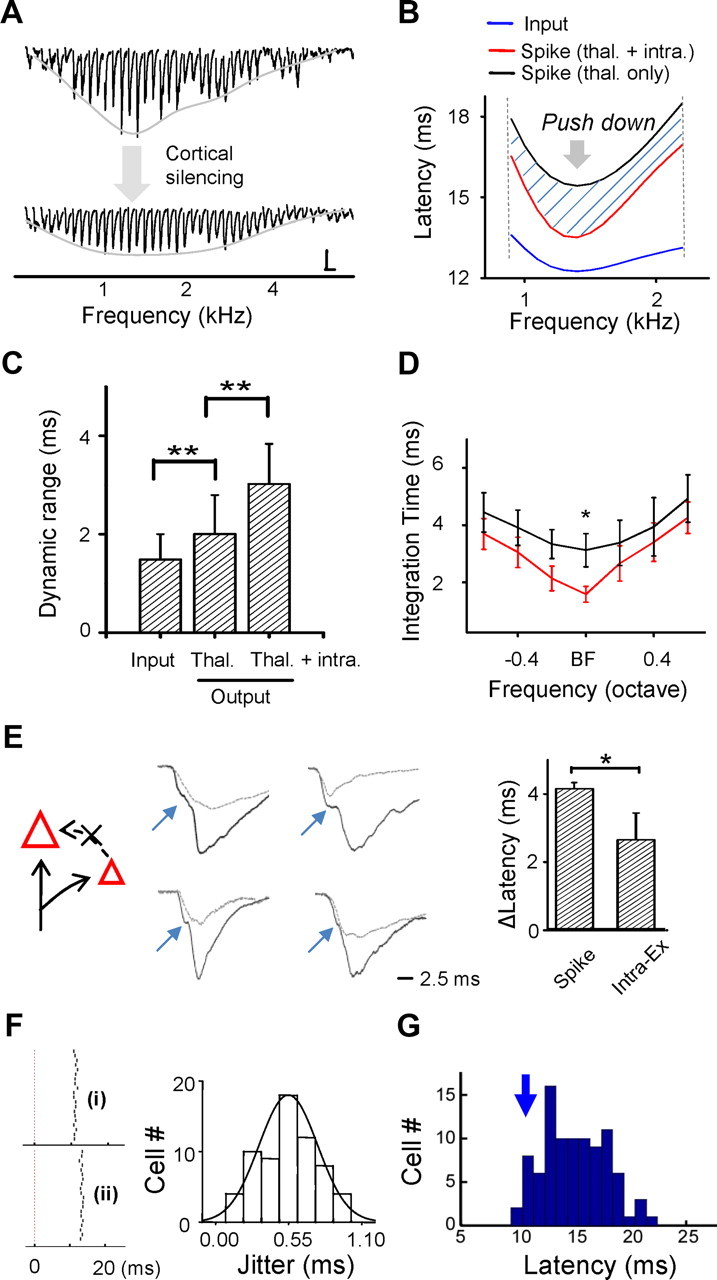
Contribution of thalamocortical and intracortical excitatory inputs to spike latency tuning. A, Excitatory responses to 70 dB tones of various frequencies before and after cortical silencing in an example neuron. The gray curve depicts the tuning curve of synaptic strength. Calibration: 100 pA, 100 ms. B, Smoothed tuning curves of thalamocortical input latency (blue) and spike latency derived from the thalamocortical input alone (black) and that from the total excitatory input (red) within the estimated spiking frequency range. C, Average dynamic range of input latency and of spike latency based on the thalamocortical input only and that based on the total excitatory input. D, Average tuning curves of integration time derived from the total excitatory input (red) and from the thalamocortical input only (black). Whiskers indicate SE. E, Left, Schematic drawing shows that input from other cortical excitatory neurons (represented by the smaller triangle) is eliminated after cortical silencing. Middle, Average excitatory responses to BF tones before (black) and after (gray) cortical silencing in four example cells. Blue arrow points to the “kink” in the response trace before cortical silencing, which indicates the arrival of a fast intracortical excitatory input. Right, Latency of the first spike and of the second excitatory component relative to the onset of excitation. Error bars indicate SD. *p < 0.01; **p < 0.001 (paired t test, n = 10). F, Left, Raster plot of spike time in response to repeated 70 dB BF tones (20 trials) for two example cells. Right, Distribution of jitters of first spike latency for neurons tested. G, Distribution of first spike latencies within 93 neurons recorded in the middle layers with cell-attached recordings.

Results from a total of 10 cells were summarized. We found that the dynamic range of thalamocortical input latency was quite narrow (1.5 ± 0.5 ms, mean ± SD) (Fig. 5C). When spikes were generated from thalamocortical inputs alone, the dynamic range of spike latency was slightly broader than that of input latency (2.0 ± 0.8 ms). When the intracortical excitation was included, the dynamic range of spike latency was further broadened to 3.1 ± 0.8 ms (Fig. 5C), doubling the dynamic range of input latency. Again, this can be attributed to a frequency-dependent modulation of integration time. Comparing tuning curves of integration time resulting from the thalamocortical input alone and from the total excitatory input (Fig. 5D, black and red curves, respectively), it is clear that the intracortical excitatory input generally reduced the integration time, but the effect was most prominent at the optimal frequency. Thus, by selectively shortening the integration time at/near the optimal frequency, the intracortical excitatory input expands the dynamic range of spike latency and sharpens its frequency tuning.

Since intracortical excitatory inputs rely on firing of cortical excitatory neurons, some of these neurons have to spike very fast for their outputs to affect other cells' spiking. We then carefully examined excitatory response traces before and after cortical silencing. As shown in Figure 5E, the excitatory response traces often exhibited a “kink” in the rising phase, which disappeared after cortical silencing. This suggests that the earliest excitatory component can be attributed to the direct thalamic input, whereas the second excitatory component that generates the kink is likely due to intracortical input. On average, the onset of this second component is 2.6 ± 0.7 ms (mean ± SD) after the initial onset of the excitatory response, while that of the first evoked spike is 4.2 ± 0.3 ms (p < 0.05, t test). Therefore the intracortical excitatory input (at least the earliest part) to the recorded cells arrived significantly earlier than their spike onset, and was able to contribute to the modulation of spike timing. The second excitatory component is unlikely attributed to random early firing of some cortical neurons due to membrane fluctuations, since spike timing of individual neurons was fairly precise, with jitters mostly around half a millisecond (Fig. 5F) (Wehr and Zador, 2003). In our intracellularly recorded neurons, the average spike latency was 14.34 ± 0.42 ms (mean ± SD, n = 15). However, loose-patch recordings from a much larger population of middle layer neurons with regular-spiking properties showed that a small portion of neurons did spike significantly earlier (Fig. 5G, arrow). It is possible that this population of early spiking neurons provide fast feedforward excitation to pyramidal neurons, which are more commonly encountered in our blind whole-cell recordings.

Impacts of tuning pattern of synaptic inputs on integration time

Both intracortical excitatory and inhibitory inputs enhance spike latency tuning through a frequency-dependent differential modulation of integration time. We next examined how such differential modulation is determined by the tuning properties of intracortical excitatory and inhibitory inputs. We derived the intracortical excitatory input by subtracting the isolated thalamocortical input from the total excitatory input. Comparing the average tuning curves of synaptic strength, we found that the intracortical excitatory input shared the same optimal frequency as the thalamocortical input, but was much more sharply tuned (Fig. 6A), consistent with the previous report (Liu et al., 2007). As the intracortical excitatory input was strongest at the optimal frequency, it would shorten spike latency significantly more at the optimal frequency than at off-optimal frequencies. In addition, as reported previously (Wu et al., 2008; Sun et al., 2010), the inhibitory input was significantly more broadly than the excitatory input (Fig. 6B). As such, inhibition as relative to excitation was stronger at off-optimal than the optimal frequency. This would result in a greater increase of integration time at off-optimal frequencies.

We next simulated the generation of spike latency tuning with the neuron model when manipulating the tuning patterns of intracortical excitatory and inhibitory inputs. The temporal profiles of simulated excitatory and inhibitory inputs (Fig. 6C) and the tuning patterns of synaptic strength were fits of our experimental data (see Materials and Methods). We first examined separate effects of intracortical excitation and inhibition on integration time. As shown by Figure 6D, with a fixed thalamocortical input, integration time changed monotonically as the intracortical excitation or inhibition increased in strength: it shortened with the increase of intracortical excitation and prolonged with the increase of cortical inhibition. In other words, any frequency-dependent variation of strength of intracortical excitatory or inhibitory inputs would result in a differential impact on integration time across different frequencies. We next examined the impact of intracortical excitation of two possible tuning patterns: similarly tuned as the thalamocortical input (“cotuned”) and more sharply tuned than the thalamocortical input (“sharp”) as observed experimentally. While the cotuned and sharply tuned intracortical excitation equally shortened integration time at the optimal frequency, at off-optimal frequencies the sharply tuned intracortical excitation affected the integration time much less effectively than the cotuned intracortical excitation (Fig. 6E, top). Compared to the spike latency tuning generated by the thalamocortical input alone, the sharply tuned intracortical excitation increased the dynamic range of spike latency, whereas the cotuned intracortical excitation decreased it (Fig. 6E, bottom). Additionally, we tested two inhibitory tuning patterns: similarly tuned as excitation (“cotuned”) and more broadly tuned than excitation (“broad”), as observed experimentally. Both the cotuned and broadly tuned inhibition significantly prolonged integration time at off-optimal frequencies, with the broadly tuned inhibition more effective in exerting this effect (Fig. 6F). The broadly tuned inhibition together with the sharply tuned intracortical excitation profoundly broadened the dynamic range of latency tuning by a factor of ∼3 (Fig. 6F, bottom, compare blue curve, gray dashed curve). These simulation results demonstrate that sharply tuned intracortical excitatory inputs and broadly tuned inhibitory inputs can be two effective strategies for increasing dynamic range of integration time.

A circuit model for generating latency tuning

The synaptic integration in the single-neuron model does not address how the spike latency tuning is generated in a large thalamocortical network or whether latency tuning of thalamic inputs is absolutely required. In addition, whether the spike latency tuning can be preserved under relatively high levels of background activity is unknown. To address these issues, we used a thalamocortical network model (see Materials and Methods). The model contained four layers of neurons (Fig. 7A). The layers of pyramidal neurons, excitatory interneurons, and inhibitory interneurons all receive direct thalamic inputs. The excitatory interneurons and inhibitory interneurons provide feedforward excitation and feedforward inhibition to the pyramidal neurons, respectively. With this circuit model, we correctly produced the sequence of events in the pyramidal neurons: the broadly tuned thalamic input arrived first, and the sharply tuned intracortical excitatory input and broadly tuned inhibitory input followed by ∼2 ms (Fig. 7B). The model also largely replicated the contribution of each synaptic component to the generation of spike latency tuning. The thalamic input alone resulted in weak spike latency tuning with a dynamic range of ∼1 ms over one octave (Fig. 7C, green). The sharply tuned input from excitatory interneurons slightly increased the sharpness of spike latency tuning by shortening the integration time at the optimal frequency more than at far away frequencies (Fig. 7C, red). The broadly tuned inhibition then profoundly sharpened the spike latency tuning by prolonging the integration time preferably at frequencies far away from the optimal frequency (Fig. 7C, blue). Together, the intracortical inputs expand the dynamic range of spike latency to >3 ms over 1 octave (Fig. 7C, bottom).

Figure 7.

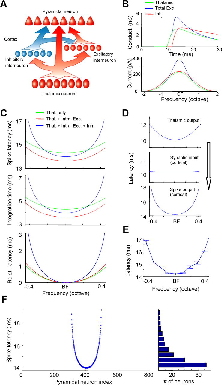
A thalamocortical network model. A, Schematic drawing of the network configuration. The pyramidal neurons in layer 4 receive input from three sources: direct input from thalamic neurons and feedforward intracortical excitation and inhibition from cortical excitatory and inhibitory interneurons driven by thalamic afferents. B, Top, Temporal profiles of synaptic conductances in the pyramidal neuron. The amplitudes are for the responses to the BF tone. Bottom, Tuning curves of peak synaptic currents evoked under simulated voltage-clamp conditions (at −70mV for excitatory currents and 0 mV for inhibitory currents). C, Top, Spike latency tuning for the pyramidal neuron under three conditions: with the thalamic input only (green), with combined thalamic and intracortical excitatory inputs (red), and with all inputs including inhibition (blue). Middle, Tuning of integration time under the three conditions. Bottom, Tuning of relative spike latency. D, Relay of latency tuning from the thalamus to the cortex. Top, Spike latency tuning for individual thalamic neurons defined in the model. Middle, Latency tuning of the aggregate thalamic input received by individual pyramidal neurons in layer 4. Bottom, Spike latency tuning of individual pyramidal neurons. E, Spike latency tuning of a pyramidal neuron with 20 Hz background activity added to all cortical neurons. Data are averaged from 100 running trials. Whiskers indicate SE. F, Spike latencies of all pyramidal neurons (800 neurons) in response to a middle-frequency tone in the network model. Neurons are indexed according to their characteristic frequency. Right, Histogram for the distribution of first spike latencies. Bin size, 0.5ms.

We next examined whether the latency tuning of thalamic inputs was necessary for the generation of cortical spike latency tuning. As shown in Figure 7D, although outputs of individual thalamic neurons exhibited a clear latency tuning, the aggregate input to each pyramidal neuron had a flat latency tuning. This result supports our original hypothesis that the convergence of thalamic inputs can lead to a degradation of input latency tuning (Fig. 1A). Even though the input latency tuning was flat, the output of the pyramidal neurons exhibited sharp latency tuning. This result strongly suggests that a significant part of spike latency tuning can be created by local cortical circuits.

Finally, we examined the impact of spontaneous firing activity (noise) on the generation of latency tuning with the network model. Random background firing of various levels was added to cortical neurons (Materials and Methods). As shown in Figure 7E as an example, in the presence of 20 Hz background activity, which is above the level of typical background activity of A1 neurons (Wu et al., 2008), latency tuning of an individual neuron could be largely preserved, although the jitter of spike timing did increase especially at off-optimal frequencies. Previous studies suggest that in the absence of an external synch signal indicating the stimulus onset, the brain network may pool spike times carried by individual neurons to generate an internal time reference (Stecker and Middlebrooks, 2003; Chase and Young 2007). Here in our network model, we observed that for a given tone stimulus, the distribution of spike latencies of pyramidal neurons was skewed, with a large population of neurons responding almost synchronously with a short delay (Fig. 7F). The detection of such synchronous firing can produce an internal synch signal, which may alleviate the deleterious effect of spontaneous spikes not related to the stimulus onset.

Discussion

First spike latency has been thought as a potential effective coding strategy, for which a sufficiently broad dynamic range should be essential for a sensitive and precise representation of stimulus attributes such as sound frequency. In this study, we demonstrate in layer 4 pyramidal neurons that within the frequency range for spiking response, the dynamic range of latency tuning is ∼1 ms for the input, while it is increased to ∼4 ms for the spike output.

We propose a simple model for the generation of sharp spike latency tuning (Fig. 8). The spike latency tuning of auditory cortical pyramidal neurons is not simply inherited from the latency information carried by convergent thalamocortical afferents, but is mainly generated de novo by local synaptic circuits. This is achieved through a fine-tuning of the integration time for spike generation. Due to the differential tuning of input strength between thalamocortical and intracortical excitatory inputs as well as between inhibitory and total excitatory inputs, two antagonistic effects are generated concurrently: the sharply tuned intracortical excitation shortens the integration time most robustly at the optimal frequency, while the broadly tuned inhibition prolongs it most powerfully at off-optimal frequencies. This “push-and-pull” modulation establishes spike latency tuning by greatly expanding its dynamic range. Under these mechanisms an initial tuning of input latency is not absolutely required for the creation of spike latency tuning.

Figure 8.

A schematic model for generating spike latency tuning in layer 4. A, Top, Tuning of onset latency for the summed thalamocortical input. Bottom, Circuit diagram showing the convergence of thalamic inputs. B, Left, Integration time is shortened and prolonged by intracortical excitation and inhibition, respectively. The red dashed line represents the spike threshold. Right, Impacts of intracortical excitation and inhibition on spike latencies (black curves). The dashed curve depicts the spike latency tuning resulting from the thalamocortical input alone. C, Top, The final output latency tuning (solid) compared to that generated by the thalamic input alone (dashed). Bottom, Circuit diagram. CX, Cortex.

Contribution of feedforward inhibition to latency tuning

Our results strongly support a significant contribution of feedforward inhibition to spike latency tuning of pyramidal neurons. The onset of inhibition is at ∼2 ms following the onset of excitation, but before the occurrence of the first evoked spike, which is at least 4 ms after the excitatory onset. Thus, the early inhibitory input is feedforward and can only come from inhibitory neurons that spike earlier than pyramidal neurons. We reported previously that fast-spiking neurons, the major type of inhibitory neurons in layer 4 (Kawaguchi and Kubota, 1997), spike significantly earlier than pyramidal neurons (Wu et al., 2008). They likely receive direct thalamic input since the onset of depolarizing responses in these neurons is as early as pyramidal cells (Wu et al., 2008). These fast-spiking neurons are the most likely inhibitory neurons that provide feedforward inhibition to pyramidal cells (Schiff and Reyes, 2012). The frequency tuning of inhibitory input strength is broader than that of excitation. Besides sharpening the tuning of spike rate response through an analogous lateral inhibition effect (Wu et al., 2008), the more broadly tuned inhibition sharpens spike latency tuning by imposing larger E/I ratios at receptive field peripheries. There the already long integration time will be further prolonged, resulting in a large expansion of dynamic range of spike latency. The more broadly tuned inhibition has an advantage over cotuned inhibition in sharpening spike latency tuning, as shown by our modeling results (Fig. 6F).

The potential sources of intracortical excitation

In this study we have intended to isolate the intracortical excitatory input using our previously established cortical silencing method (Liu et al., 2007). The effectiveness and specificity of this method have been further verified by two more recent studies (Khibnik et al., 2010; Zhang et al., 2011) demonstrating that the presynaptic transmission can be well preserved after the mixture application. The comparison of temporal profiles of evoked excitatory responses before and after the cortical silencing revealed a distinct excitatory component starting at ∼2 ms after the initial onset of excitation. Although nonspecific effects of the mixture application [e.g., increased membrane leakage, discussed by Liu et al. (2007), supplemental information] cannot be totally excluded, the specific changes in excitatory responses after the mixture application in both the temporal (Fig. 5E) and frequency (Fig. 6A) domains support a specific elimination of excitation of intracortical sources. Application of the mixture will also disrupt intracortical oscillatory activity reported to govern cellular excitability (Barth and MacDonald, 1996; Metherate and Cruikshank, 1999; Sukov and Barth, 2001; Oswald et al., 2009) and inputs associated with oscillations. Although this may contribute to the reduction of the delayed excitatory response, the temporal feature of the response (with an ∼2 ms delay relative to the initial excitatory onset) is difficult to be explained by the known frequency of oscillations (i.e., 30–80 Hz gamma oscillations).

The tone-evoked intracortical excitatory inputs can be attributed to feedforward, feedback, or recurrent connections. In principle, feedback and recurrent inputs would arrive later than the occurrence of the first spike of layer 4 pyramidal neurons, and would be unable to affect its timing. If recurrent connections are prominent among pyramidal neurons, we would expect to see a distinct excitatory component occurring at ∼4 ms after the initial onset of excitation, when the majority of pyramidal neurons are expected to fire. This was not evident. In addition, the small jitter of spike timing of individual pyramidal neurons (Fig. 5F) reduces the possibility that a random subgroup of pyramidal neurons fire early, due to fluctuations, to modulate spiking of other pyramidal neurons through recurrent connections. Based on the above reasoning, we raise a possibility that the early excitatory intracortical component is due to a disynaptic relay from some excitatory neurons that spike stereotypically earlier than the recorded pyramidal cells (i.e., feedforward circuit).

Although blind loose-patch recordings suggested a small population of early spiking neurons (Fig. 5G), the identities of these presumptive excitatory relay neurons are elusive. Besides well characterized pyramidal neurons in layer 4 of the auditory cortex, previous studies have also observed a small number of spiny stellate cells (Winer, 1984; Rose and Metherate, 2005; Richardson et al., 2009). Their number could be underestimated since they are reported to be resistant to Golgi impregnation and difficult to sample with intracellular recordings (Y. Wang et al., 2010). Can these stellate cells provide feedforward excitation to pyramidal neurons? The auditory response properties of these neurons have not been characterized. Current-patch recording methods (in vivo and ex vivo) all show sampling bias toward large pyramidal neurons (Tan et al., 2004; Wu et al., 2008; Richardson et al., 2009). Future technical improvements are needed to identify and record from spiny stellate neurons in vivo as to test whether they can serve as the postulated excitatory interneurons.

Issues on latency coding

It remains under debate whether and how spike latency is used by the nervous system to code for stimulus attributes (deCharms and Zador 2000; Laurent et al., 2001; Chase and Young 2007). Spike latency has its unique advantage of carrying information, but there are challenges to extracting the information. A major challenge is that the brain has no access to the external stimulus onset (i.e., the external synch signal) to determine latency, and thus an internally generated time reference is necessary. Several sources of internal time reference have been proposed, including large-scale oscillations (Hopfield, 1995), local field potentials (Eggermont, 1998), and population onsets (Stecker and Middlebrooks, 2003; Chase and Young, 2007). In our modeling study, we found that for any given tone stimulus, a large fraction of responding pyramidal neurons can fire almost simultaneously (Fig. 7E). The detection of synchronous firing of a large number of neurons may provide a population onset to which spike times of individual neurons are referenced (Chase and Young, 2007). Whether this strategy is indeed implemented by the cortical circuits remains an open question. Another issue is that the noise is often seen as being destructive to latency coding more than to rate coding. This is partly because the information in rate codes is assumed to be extracted by pooling a large number of neurons together, while with latency codes, single spikes are often expected to provide sufficient information. In fact, latency codes can benefit just as much from pooling from a population of neurons (Chase and Young, 2007; Quian Quiroga and Panzeri, 2009). In addition, in the presence of a highly correlated population of neurons, the noise may be less destructive than expected, because the jitter of spike timing relative to that of other neurons may be lower than that referenced to the stimulus onset.

Finally, for spike latency to serve the coding purpose two prerequisites have to be met: (1) relatively precise spike timing upon each stimulus presentation and (2) a broad dynamic range of spike latency to represent parameter values with sufficient resolution. Previous studies have demonstrated that the precision of spike timing is ensured by inhibition that follows excitation with a brief delay (Wehr and Zador, 2003). The current study further reveals the synaptic mechanisms for expanding the dynamic range of spike latency. The submillisecond precision (Fig. 5F) combined with a 4 ms dynamic range may be sufficient for implementing latency codes. As the revealed synaptic mechanisms highly depend on the tuning properties of synaptic strength, our study suggests an efficient strategy for converting information spatially coded in the distribution of synaptic strength into temporal representation. The thalamocortical-like circuit may be an elementary circuit that can fulfill this function.

References

- Barth DS, MacDonald KD. Thalamic modulation of high-frequency oscillating potentials in auditory cortex. Nature. 1996;383:78–81. doi: 10.1038/383078a0. [DOI] [PubMed] [Google Scholar]
- Borg-Graham LJ, Monier C, Frégnac Y. Visual input evokes transient and strong shunting inhibition in visual cortical neurons. Nature. 1998;393:369–373. doi: 10.1038/30735. [DOI] [PubMed] [Google Scholar]
- Brugge JF, Reale RA, Jenison RL, Schnupp J. Auditory cortical spatial receptive fields. Audiol Neurootol. 2001;6:173–177. doi: 10.1159/000046827. [DOI] [PubMed] [Google Scholar]
- Bruno RM, Sakmann B. Cortex is driven by weak but synchronously active thalamocortical synapses. Science. 2006;312:1622–1627. doi: 10.1126/science.1124593. [DOI] [PubMed] [Google Scholar]
- Butts DA, Weng C, Jin J, Yeh CI, Lesica NA, Alonso JM, Stanley GB. Temporal precision in the neural code and the time scales of natural vision. Nature. 2007;449:92–95. doi: 10.1038/nature06105. [DOI] [PubMed] [Google Scholar]
- Chase SM, Young ED. First-spike latency information in single neurons increases when referenced to population onset. Proc Natl Acad Sci U S A. 2007;104:5175–5180. doi: 10.1073/pnas.0610368104. [DOI] [PMC free article] [PubMed] [Google Scholar]
- Chen X, Leischner U, Rochefort NL, Nelken I, Konnerth A. Functional mapping of single spines in cortical neurons in vivo. Nature. 2011;475:501–505. doi: 10.1038/nature10193. [DOI] [PubMed] [Google Scholar]
- Chung S, Ferster D. Strength and orientation tuning of the thalamic input to simple cells revealed by electrically evoked cortical suppression. Neuron. 1998;20:1177–1189. doi: 10.1016/s0896-6273(00)80498-5. [DOI] [PubMed] [Google Scholar]
- deCharms RC, Zador A. Neural representation and the cortical code. Annu Rev Neurosci. 2000;23:613–647. doi: 10.1146/annurev.neuro.23.1.613. [DOI] [PubMed] [Google Scholar]
- de la Rocha J, Marchetti C, Schiff M, Reyes AD. Linking the response properties of cells in auditory cortex with network architecture: cotuning versus lateral inhibition. J Neurosci. 2008;28:9151–9163. doi: 10.1523/JNEUROSCI.1789-08.2008. [DOI] [PMC free article] [PubMed] [Google Scholar]
- DeWeese MR, Wehr M, Zador AM. Binary spiking in auditory cortex. J Neurosci. 2003;23:7940–7949. doi: 10.1523/JNEUROSCI.23-21-07940.2003. [DOI] [PMC free article] [PubMed] [Google Scholar]
- DiMatteo I, Genovese C, Kass R. Bayesian curve-fitting with free-knot splines. Biometrika. 2001;88:1055–1071. [Google Scholar]
- Douglas RJ, Martin KA. Neuronal circuits of the neocortex. Annu Rev Neurosci. 2004;27:419–451. doi: 10.1146/annurev.neuro.27.070203.144152. [DOI] [PubMed] [Google Scholar]
- Eggermont JJ. Azimuth coding in primary auditory cortex of the cat. II. Relative latency and interspike interval representation. J Neurophysiol. 1998;80:2151–2161. doi: 10.1152/jn.1998.80.4.2151. [DOI] [PubMed] [Google Scholar]
- Elhilali M, Fritz JB, Klein DJ, Simon JZ, Shamma SA. Dynamics of precise spike timing in primary auditory cortex. J Neurosci. 2004;24:1159–1172. doi: 10.1523/JNEUROSCI.3825-03.2004. [DOI] [PMC free article] [PubMed] [Google Scholar]
- Furukawa S, Middlebrooks JC. Cortical representation of auditory space: information-bearing features of spike patterns. J Neurophysiol. 2002;87:1749–1762. doi: 10.1152/jn.00491.2001. [DOI] [PubMed] [Google Scholar]
- Gollisch T, Meister M. Rapid neural coding in the retina with relative spike latencies. Science. 2008;319:1108–1111. doi: 10.1126/science.1149639. [DOI] [PubMed] [Google Scholar]
- Hackett TA, Barkat TR, O'Brien BM, Hensch TK, Polley DB. Linking topography to tonotopy in the mouse auditory thalamocortical circuit. J Neurosci. 2011;31:2983–2995. doi: 10.1523/JNEUROSCI.5333-10.2011. [DOI] [PMC free article] [PubMed] [Google Scholar]
- Heil P. Auditory cortical onset responses revisited. I. First-spike timing. J Neurophysiol. 1997;77:2616–2641. doi: 10.1152/jn.1997.77.5.2616. [DOI] [PubMed] [Google Scholar]
- Heil P. First-spike latency of auditory neurons revisited. Curr Opin Neurobiol. 2004;14:461–467. doi: 10.1016/j.conb.2004.07.002. [DOI] [PubMed] [Google Scholar]
- Hines M. In: In neural systems: analysis and modeling. Eeckman F, editor. Norwell, MA: Kluwer; 1993. pp. 127–136. [Google Scholar]
- Hopfield JJ. Pattern recognition computation using action potential timing for stimulus representation. Nature. 1995;376:33–36. doi: 10.1038/376033a0. [DOI] [PubMed] [Google Scholar]
- Johansson RS, Birznieks I. First spikes in ensembles of human tactile afferents code complex spatial fingertip events. Nat Neurosci. 2004;7:170–177. doi: 10.1038/nn1177. [DOI] [PubMed] [Google Scholar]
- Junek S, Kludt E, Wolf F, Schild D. Olfactory coding with patterns of response latencies. Neuron. 2010;67:872–884. doi: 10.1016/j.neuron.2010.08.005. [DOI] [PubMed] [Google Scholar]
- Kawaguchi Y, Kubota Y. GABAergic cell subtypes and their synaptic connections in rat frontal cortex. Cereb Cortex. 1997;7:476–486. doi: 10.1093/cercor/7.6.476. [DOI] [PubMed] [Google Scholar]
- Khibnik LA, Cho KK, Bear MF. Relative contribution of feedforward excitatory connections to expression of ocular dominance plasticity in layer 4 of visual cortex. Neuron. 2010;66:493–500. doi: 10.1016/j.neuron.2010.04.012. [DOI] [PMC free article] [PubMed] [Google Scholar]
- Kitzes LM, Gibson MM, Rose JE, Hind JE. Initial discharge latency and threshold considerations for some neurons in cochlear nuclear complex of the cat. J Neurophysiol. 1978;41:1165–1182. doi: 10.1152/jn.1978.41.5.1165. [DOI] [PubMed] [Google Scholar]
- Laurent G, Stopfer M, Friedrich RW, Rabinovich MI, Volkovskii A, Abarbanel HD. Odor encoding as an active, dynamical process: experiments, computation, and theory. Annu Rev Neurosci. 2001;24:263–297. doi: 10.1146/annurev.neuro.24.1.263. [DOI] [PubMed] [Google Scholar]
- Liang F, Yang W, Zheng X, Wang X, Tan X, Zhang F, Xiao Z. Response property of inferior collicular neurons inherited from peripheral origin in mouse. Brain Res. 2011;1369:46–59. doi: 10.1016/j.brainres.2010.11.011. [DOI] [PubMed] [Google Scholar]
- Liu BH, Wu GK, Arbuckle R, Tao HW, Zhang LI. Defining cortical frequency tuning with recurrent excitatory circuitry. Nat Neurosci. 2007;10:1594–1600. doi: 10.1038/nn2012. [DOI] [PMC free article] [PubMed] [Google Scholar]
- Metherate R, Cruikshank SJ. Thalamocortical inputs trigger a propagating envelope of gamma-band activity in auditory cortex in vitro. Exp Brain Res. 1999;126:160–174. doi: 10.1007/s002210050726. [DOI] [PubMed] [Google Scholar]
- Okun M, Lampl I. Instantaneous correlation of excitation and inhibition during ongoing and sensory-evoked activities. Nat Neurosci. 2008;11:535–537. doi: 10.1038/nn.2105. [DOI] [PubMed] [Google Scholar]
- Oswald AM, Doiron B, Rinzel J, Reyes AD. Spatial profile and differential recruitment of GABAB modulate oscillatory activity in auditory cortex. J Neurosci. 2009;29:10321–10334. doi: 10.1523/JNEUROSCI.1703-09.2009. [DOI] [PMC free article] [PubMed] [Google Scholar]
- Panzeri S, Petersen RS, Schultz SR, Lebedev M, Diamond ME. The role of spike timing in the coding of stimulus location in rat somatosensory cortex. Neuron. 2001;29:769–777. doi: 10.1016/s0896-6273(01)00251-3. [DOI] [PubMed] [Google Scholar]
- Quian Quiroga R, Panzeri S. Extracting information from neuronal populations: information theory and decoding approaches. Nat Rev Neurosci. 2009;10:173–185. doi: 10.1038/nrn2578. [DOI] [PubMed] [Google Scholar]
- Richardson RJ, Blundon JA, Bayazitov IT, Zakharenko SS. Connectivity patterns revealed by mapping of active inputs on dendrites of thalamorecipient neurons in the auditory cortex. J Neurosci. 2009;29:6406–6417. doi: 10.1523/JNEUROSCI.0258-09.2009. [DOI] [PMC free article] [PubMed] [Google Scholar]
- Rose HJ, Metherate R. Auditory thalamocortical transmission is reliable and temporally precise. J Neurophysiol. 2005;94:2019–2030. doi: 10.1152/jn.00860.2004. [DOI] [PubMed] [Google Scholar]
- Schiff ML, Reyes AD. Characterization of thalamocortical responses of regular-spiking and fast-spiking neurons of the mouse auditory cortex in vitro and in silico. J Neurophysiol. 2012;107:1476–1488. doi: 10.1152/jn.00208.2011. [DOI] [PMC free article] [PubMed] [Google Scholar]
- Stecker GC, Middlebrooks JC. Distributed coding of sound locations in the auditory cortex. Biol Cybern. 2003;89:341–349. doi: 10.1007/s00422-003-0439-1. [DOI] [PubMed] [Google Scholar]
- Sukov W, Barth DS. Cellular mechanisms of thalamically evoked gamma oscillations in auditory cortex. J Neurophysiol. 2001;85:1235–1245. doi: 10.1152/jn.2001.85.3.1235. [DOI] [PubMed] [Google Scholar]
- Sun YJ, Wu GK, Liu BH, Li P, Zhou M, Xiao Z, Tao HW, Zhang LI. Fine-tuning of pre-balanced excitation and inhibition during auditory cortical development. Nature. 2010;465:927–931. doi: 10.1038/nature09079. [DOI] [PMC free article] [PubMed] [Google Scholar]
- Tan AY, Zhang LI, Merzenich MM, Schreiner CE. Tone-evoked excitatory and inhibitory synaptic conductances of primary auditory cortex neurons. J Neurophysiol. 2004;92:630–643. doi: 10.1152/jn.01020.2003. [DOI] [PubMed] [Google Scholar]
- Tan X, Wang X, Yang W, Xiao Z. First spike latency and spike count as functions of tone amplitude and frequency in the inferior colliculus of mice. Hear Res. 2008;235:90–104. doi: 10.1016/j.heares.2007.10.002. [DOI] [PubMed] [Google Scholar]
- Wang HP, Spencer D, Fellous JM, Sejnowski TJ. Synchrony of thalamocortical inputs maximizes cortical reliability. Science. 2010;328:106–109. doi: 10.1126/science.1183108. [DOI] [PMC free article] [PubMed] [Google Scholar]
- Wang X, Lu T, Bendor D, Bartlett E. Neural coding of temporal information in auditory thalamus and cortex. Neuroscience. 2008;157:484–494. doi: 10.1016/j.neuroscience.2008.07.050. [DOI] [PubMed] [Google Scholar]
- Wang Y, Brzozowska-Prechtl A, Karten HJ. Laminar and columnar auditory cortex in avian brain. Proc Natl Acad Sci U S A. 2010;107:12676–12681. doi: 10.1073/pnas.1006645107. [DOI] [PMC free article] [PubMed] [Google Scholar]
- Wehr M, Zador AM. Balanced inhibition underlies tuning and sharpens spike timing in auditory cortex. Nature. 2003;426:442–446. doi: 10.1038/nature02116. [DOI] [PubMed] [Google Scholar]
- Winer JA. Anatomy of layer IV in cat primary auditory cortex (AI) J Comp Neurol. 1984;224:535–567. doi: 10.1002/cne.902240405. [DOI] [PubMed] [Google Scholar]
- Wu GK, Li P, Tao HW, Zhang LI. Nonmonotonic synaptic excitation and imbalanced inhibition underlying cortical intensity tuning. Neuron. 2006;52:705–715. doi: 10.1016/j.neuron.2006.10.009. [DOI] [PMC free article] [PubMed] [Google Scholar]
- Wu GK, Arbuckle R, Liu BH, Tao HW, Zhang LI. Lateral sharpening of cortical frequency tuning by approximately balanced Inhibition. Neuron. 2008;58:132–143. doi: 10.1016/j.neuron.2008.01.035. [DOI] [PMC free article] [PubMed] [Google Scholar]
- Zhang LI, Tan AY, Schreiner CE, Merzenich MM. Topography and synaptic shaping of direction selectivity in primary auditory cortex. Nature. 2003;424:201–205. doi: 10.1038/nature01796. [DOI] [PubMed] [Google Scholar]
- Zhang M, Liu Y, Wang SZ, Zhong W, Liu BH, Tao HW. Functional elimination of excitatory feedforward inputs underlies developmental refinement of visual receptive fields in zebrafish. J Neurosci. 2011;31:5460–5469. doi: 10.1523/JNEUROSCI.6220-10.2011. [DOI] [PMC free article] [PubMed] [Google Scholar]
- Zhou Y, Liu BH, Wu GK, Kim YJ, Xiao Z, Tao HW, Zhang LI. Preceding inhibition silences layer 6 neurons in auditory cortex. Neuron. 2010;65:706–717. doi: 10.1016/j.neuron.2010.02.021. [DOI] [PMC free article] [PubMed] [Google Scholar]