Interfacial thermodynamics of confined water near molecularly rough surfaces

Abstract

We study the effects of nanoscopic roughness on the interfacial free energy of water confined between solid surfaces. SPC/E water is simulated in confinement between two infinite planar surfaces that differ in their physical topology: one is smooth and the other one is physically rough on a nanometer length scale. The two thermodynamic ensembles considered, with constant pressure either normal or parallel to the walls, correspond to different experimental conditions. We find that molecular-scale surface roughness significantly increases the solid-liquid interfacial free energy compared to the smooth surface. For our surfaces with a water-wall interaction energy minimum of −1.2 kcal/mol, we observe a transition from a hydrophilic surface to a hydrophobic surface at a roughness amplitude of about 3 Å and a wave length of 11.6 Å, with the interfacial free energy changing sign from negative to positive. In agreement with previous studies of water near hydrophobic surfaces, we find an increase in the isothermal compressibility of water with increasing surface roughness. Interestingly, average measures of the water density and hydrogen-bond number do not contain distinct signatures of increased hydrophobicity. In contrast, a local analysis indicates transient dewetting of water in the valleys of the rough surface, together with a significant loss of hydrogen bonds, and a change in the dipole orientation toward the surface. These microscopic changes in the density, hydrogen bonding, and water orientation contribute to the large increase in the interfacial free energy, and the change from a hydrophilic to a hydrophobic character of the surface.

1 Introduction

Water plays a central role in many of the biomolecular self-assembly processes, including the folding of proteins and the formation of lipid membranes.^1–10 In key steps of these biomolecular processes, water is often highly confined,¹¹ reduced for instance to a few layers of water molecules between the extended surfaces of large macromolecules. Considering the diversity in the chemical and physical topology of these surfaces, the interfacial behavior of water in a cellular environment will depend sensitively on the details of the confining surfaces. The wetting behavior of surfaces and its dependence on the physical and chemical nanostructure are also technologically relevant, for instance in the development of low-friction fluid flow channels.^11–13

Quantitative experimental studies of water at interfaces are highly challenging,^14–17 and roughness can be a relevant parameter.¹⁸ Recent advances in both theory and experiments⁹ have re-invigorated the interest in the molecular underpinning of the hyydrophobic effect and the behavior of water near surfaces. Water confined between a “Janus interface” of adjoining hydrophobic and hydrophilic surfaces was found to fluctuate significantly during shear deformations.¹⁹ This observation raises several interesting questions about water near heterogeneous surfaces and how local patchiness (wetting versus nonwetting) may affect hydrophobicity and microscopic density fluctuations.²⁰ To find answers to at least some of these questions, molecular simulations can complement the laboratory experiments because in the simulations surface details can be controlled precisely and molecular information can be obtained directly.

Previous theoretical and simulation studies have typically focused on the structure, thermodynamics, and dynamics of water confined between idealized smooth surfaces,^21–32 between atomistic surfaces,^33–37 within carbon nanotubes,¹² and between realistic protein-like surfaces.^38,39 These studies have vastly improved our molecular-level understanding of the expected changes in the water behavior due to confinement and the presence of hydrophilic versus hydrophobic surfaces.

In a laboratory experiment, one way to characterize surfaces as hydrophilic or hydrophobic is to measure the macroscopic contact angle of small water droplets on these surfaces. Recent molecular simulation studies have used a microscopic analog of the macroscopic contact angle to define the hydrophobicity of surfaces.^40–42 Giovambattista et al.⁴¹ used contact angle data to show that that water behavior can be a non-trivial function of the surface polarity. Godawat et al.⁴² studied the behavior of water near self-assembled monolayer structures with a wide range of chemistries and showed that the hydrophobicities of such surfaces as measured by contact angles can be characterized well by measures related to the water density fluctuations. We similarly saw enhanced water-density fluctuations near extended non-polar surfaces,⁴³ associated with transitions between locally wet and dry regions and resulting in a broadened liquid-vapor like interfacial density profile.

It is well known in the surface wetting literature that the physical roughness of the surface can cause the contact angle to change significantly.⁴⁴ This change is typically described by either the Cassie⁴⁵ or the Wenzel⁴⁶ model depending on the wetting properties of the smooth surface. These models are widely used to describe the effects of the mesoscopic (micron-scale) roughness of superhydrophobic surfaces, such as Lotus leafs. Much less is known on how surface roughness of the order of few molecular diameters,^47–49 which is relevant for instance to characterize protein surfaces, will affect the interfacial behavior of water.

This poor understanding of surface roughness effects on the interfacial thermodynamics also severely limits the applicability of surface-area based solvation models. Many widely used models for ligand binding and self-assembly rely on the interfacial free energy of surfaces to predict their solvation free energy.⁵⁰ However, at the molecular scale corrections should be made to the interfacial free energy to account for curvature and physical roughness.^51,52 Examples of such curvature corrections rely on the macroscopic concept of the Tolman length,⁵³ or on the microscopic observation of curvature dependent “cavity expulsion” of water.⁵⁴

To explore how molecular-scale physical roughness affects the interfacial free energy, we perform molecular dynamics simulations of water confined between walls. One of the major difficulties in performing simulations of confined water is to define the thermodynamic state of the system and to make sure that water is present in a thermodynamically stable equilibrium. Here, we consider two thermodynamic ensembles, defined by constant normal and parallel pressures (Fig. 1) at a constant temperature and with a constant number of particles. We also monitor individual components of the pressure tensor to make sure that the system is in a stable state during the entire simulation time.

Figure 1.

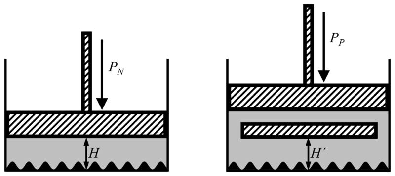
Thermodynamic ensembles. We simulate water confined between a lower rough wall and an upper smooth wall with two different constraints. (Left) Constant normal pressure P_N. Experimentally, the position of the upper surface would be controlled by a piston under constant pressure P_N. (Right) Constant parallel pressure P_P. Here the confined fluid is in equilibrium with bulk fluid at a constant pressure P_P. Note that in the two ensembles, the densities and thus the heights H and H′ will be different in general for a given number of water molecules in a box of given projected area in the xy-plane.

In our model system, the wall roughness can be changed in a controlled manner by modulating the local wall position with periodic functions of given amplitudes and wavelengths (see Fig. 2). We find that increasing wall roughness, as characterized by increasing roughness amplitude or decreasing roughness wavelength, can significantly increase the solid-liquid interfacial free energy. Roughness can even change the sign of the interfacial free energy from negative (hydrophilic) to positive (hydrophobic). We examine the microscopic origins of this change in wetting behavior in the context of hydration structure near rough walls and associated density and hydrogen bond distributions.

Figure 2.

Model system. The two confining walls are placed normal to the z-direction and a distance H apart. The physical roughness is represented by a cosine function, eqs. 1 and 2, which gives rise to the wall pattern with peaks and valleys shown on the right hand side. The panel on the left shows a simplified one-dimensional cut through the peaks along the x direction. λ is the roughness wavelength, and a is the amplitude of the roughness so that the lower wall position will vary from z = 0 to 2a.

2 Models and Methods

We use a system of N_w = 1500 SPC/E water⁵⁵ molecules in a rectangular box with periodic boundary conditions applied in two directions x and y, and fixed boundary condition applied in the z-direction. The walls are represented by a coarse-grained 9-3 Lennard-Jones potential,

$$V(z)=\epsilon \left[\frac{2}{15}{\left(\frac{\sigma }{z}\right)}^9-{\left(\frac{\sigma }{z}\right)}^3\right],$$ (1)

which is frequently used to represent interactions between a fluid particle and a wall made up of 12-6 Lennard-Jones particles. Here, ε and σ are the water-wall interaction energy and distance parameters, respectively. z is the distance between the water oxygen atom and the wall surface. We use ε = 1.15 kcal/mol and σ = 0.346 nm in this work. The resulting well depth of the wall-water interaction is ≈ −1.21 kcal/mol. To represent a rough wall as shown in Figure 2, we use a periodic function of the following form,

$$z(x,y)=acos\left(\frac{2\pi x}{\lambda }\right)cos\left(\frac{2\pi y}{\lambda }\right),$$ (2)

where z(x, y) represents the wall position as a function of x- and y-coordinates. a is the roughness amplitude, and λ is the roughness wavelength, which is an integer fraction of the simulation box length in the x and y direction. The resulting interaction V [z_i − z(x_i, y_i)] of an oxygen molecule and the wall depends on all three oxygen coordinates (x_i, y_i, z_i).

The equilibrium behavior of our confined water system is obtained from molecular dynamics simulations using LAMMPS⁵⁶ in a canonical ensemble. The temperature is held constant at 300 K by using a Nosé-Hoover thermostat with a time constant of 0.5 ps. The simulation time step is 2 fs. For each state we simulate for a total time of 4 ns. The initial 2 ns are discarded as equilibration time, and the remaining 2 ns of the simulation runs are used for the final analysis. Electrostatic interactions are calculated with particle-particle particle-mesh solver. To account for non-periodicity in the z-direction we extend the simulation box to three times the height H and apply the correction proposed by Yeh and Berkowitz.⁵⁷

We calculate the solid-liquid interfacial free energy between the confined water and confining walls from the difference between normal and parallel pressures,⁵⁸

$$\gamma \equiv {\gamma }_l+{\gamma }_u={\int }_0^H(P_N-p_P(z))dz=(P_N-P_P)H,$$ (3)

where $P_P=H^{-1}{\int }_0^H{p}_P(z)dz$ is the average of the z-dependent parallel pressure p_P (z). γ_l and γ_u are the interfacial free energies per unit area (of the surface projected onto the xy-plane) between confined water and the lower and upper wall, respectively, assuming separability.

3 Results and Discussion

To calculate how the wall roughness may affect the interfacial free energy for the confined water system shown in Fig. 2, we first calculate the pressure equations of state as a function of wall distance H. The equations of state differ for the two ensembles under constant parallel and normal pressures. As our starting smooth wall system (a = 0), we use wall-oxygen interaction parameter ε = 1.15 kcal/mol and confinement length H = 16.75 Å to obtain a system close to a stable thermodynamic equilibrium and with about 4 water layers between the walls. To explore the effects of roughness, we then modulate the wall location of the lower surface according to the periodic function function in eqs. 1 and 2. Results for the interfacial free energy will be compared in states defined by conditions of 1 atm pressure in either the normal direction (P_N) or the parallel direction (P_P) (see Fig. 1).

Figure 3 (left, insets) shows the normal pressure P_N and the parallel pressure P_P as a function of H for roughness amplitudes a between 0 and 10 Å (from left to right) of the lower wall. The simulation pressures are fitted accurately by a cubic polynomial in H. The fitted equations of state allow us to find the H values for which P_N or P_P is equal to 1 atm. We then use the respective H value to evaluate the pressure component that is not kept constant, i.e., P_P (P_N = 1 atm) and P_N (P_P = 1 atm). From the cubic fits, we also calculate the isothermal compressibility κ_T = −H⁻¹(dH/dP) in both the normal and the parallel direction. The results are shown in Fig. 3 (right, bottom) where dP/dH is evaluated at P_N = 1 atm and P_P = 1 atm, respectively. We find that κ_T increases with increasing a for both constant P_N and P_P. The confined water is thus more compressible near rough surfaces. We want to point out that this is the overall behavior of the confined system and not the local behavior near a surface as studied previously by Godawat et al.⁴² and by us.⁴³ A similar increase in κ_T for confined water system was found by Giovambattista et al. ⁴¹ with decreasing surface polarity and therefore increasing surface hydrophobicity. Also, compressibility is higher for a system at constant P_N as compared with at constant P_P for a given a.

Figure 3.

Equations of state. (Left) Normal pressure P_N (top) and parallel pressure P_P (bottom) as a function of the distance H between the walls. The interfacial area A of the simulation box in the xy-plane is kept constant. The water density is thus changing with H, effectively providing us with the pressure as a function of the density. The P (H) data are shown for increasing wall roughness amplitudes a = 0, 1.5, 3, 4.5, 6, 7.5, and 10 Å (from left to right) and for a roughness wavelength λ = 11.59 Å. The symbols are the simulation data and lines are fits to a cubic polynomial. The top and bottom insets show P_P (P_N = 1 atm) and P_N (P_P = 1 atm), respectively, as a function of the wall roughness amplitude a. (Right, top) Distance H between the walls as function of the roughness amplitudes a at 1 atm pressure (squares for P_N = 1 atm, and circles for P_P = 1 atm). (Right, bottom) Isothermal compressibility κ_T as a function of the wall roughness amplitude a at 1 atm pressure (symbols as above).

Thermodynamic stability is a possible concern in simulations of confined systems. For roughness amplitudes a ≥ 7.5 Å, we find that the cubic fits to the P − H data produce multiple roots for P (H) = 1 atm. For a ≥ 7.5 Å, we thus expect phase co-existence (in a large system) between a liquid and vapor phase, or fluctuations (in a small system) between the two “phases.” For these large roughness amplitudes a ≥ 7.5 Å, the systems simulated are thus likely metastable.

The simulation systems can also be subject to mechanical instabilities. With one of the pressure components, P_N or P_P, fixed at 1 atm, the other one can be negative. As shown in Fig. 3 (left panels), P_P (P_N = 1 atm) is negative for a ≥ 3 Å, and P_N (P_P = 1 atm) is negative for a ≤ 1.5 Å. To check whether the system underwent phase separation (through the formation of nanoscale bubbles), we track the full pressure tensor, making sure that the in-plane diagonal pressure components agree, P_xx = P_yy, and that the normal pressures on the lower and upper walls are equal, P_zz,l = P_zz,u. We do not find any signatures of such deviations for all the state points considered in this work, in particular not for conditions close to 1 atm pressure in either normal or parallel direction. Also, the slope of the pressure equations of state (Fig. 3, left) is always negative, ∂P/∂H < 0, which means that the thermodynamic stability condition is satisfied (κ_T > 0; Fig. 3 right bottom). These observations together provide a sufficient reason to believe that our systems of interest are in a thermodynamic equilibrium (or at least in a metastable equilibrium) during the entire simulation times.

Figure 4 shows the interfacial free energy γ as a function of wall roughness amplitude a (left) and wavelength λ (right) under the constraints of P_N or P_P being equal to 1 atm. We find that γ changes sign with increasing wall roughness by either increasing a (with λ = 11.6 Å fixed) or decreasing λ (with a = 3 Å fixed). This change in sign means that the hydrophilic smooth surface (γ < 0) becomes hydrophobic (γ > 0) with increasing molecular scale roughness. We also find that γ has a rather strong dependence on a and this dependence is stronger for systems under the constraint of constant parallel pressure P_P. The dependence of γ on the wavelength λ for a fixed a = 3 Å is weaker than the dependence on the amplitude a (Fig. 4, right). With increasing λ, the calculated γ values drop toward the smooth-wall limit expected for λ → ∞, albeit slowly. Importantly, physical roughness of the surfaces on the length scale of a single water molecule can change the wetting behavior of confined water qualitatively from hydrophilic (γ < 0) to hydrophobic (γ > 0).

Figure 4.

Effect of wall roughness amplitude and wavelength on interfacial properties. The combined solid-liquid interfacial free energy γ between confined water and both the lower and upper walls is shown as a function of lower wall roughness amplitude a for a fixed wavelength λ = 11.6 Å (left panel) and wall roughness wavelength λ for a fixed amplitude a = 3 Å (right panel). The inset in the right panel shows the zoomed in version. The filled symbols are the γ values calculated using eq. 3 and the cubic pressure equation of state fits shown in Fig. 3. The empty symbols are the data generated using additional simulations at H values targeting P_N = 1 atm according to the equations of state.

If we assume that the interfacial free energy of the smooth wall, γ_u, is independent of the roughness of the lower wall, we can evaluate the interfacial free energy for the rough wall by subtracting the value for the smooth wall from the total free energy, γ_l(a) ≈ γ (a) − γ (a = 0)/2. We find that the interfacial free energy for the rough wall calculated in this way varies from −8.1 mN/m to +89.1 mN/m for P_P = 1 atm and from −3.6 mN/m to +41 mN/m for P_N = 1 atm.

By assuming a solid-vapor interfacial free energy of γ_SV ≈ 0 mN/m, we can use Young’s equation based on mechanical equilibrium to find the contact angle θ of SPC/E water on our rough surfaces,

$$cos\theta =\frac{{\gamma }_{SV}-{\gamma }_{SL}}{{\gamma }_{LV}},$$ (4)

where γ_SV, γ_SL, and γ_LV are the solid-vapor, solid-liquid, and liquid-vapor interfacial tensions, respectively. With a liquid-vapor interfacial tension of γ_LV = 61.3 mN/m for SPC/E water at 300 K,⁵⁹ and with γ_l(a) assumed to be equal to γ_SL and γ_SV ≈ 0, we can use eq. 4 to estimate the contact angle. At constant P_N = 1 atm, the contact angle changes from 87° for a flat interface to 132° for a = 10 Å and λ = 11.6 Å. For constant parallel pressure, a contact angle of 180° is reached just above a = 6 Å, starting from θ ≈ 82° for a flat surface. For larger amplitudes a ≥ 7.5 Å, the calculated free energy of the liquid-solid interface exceeds that of the liquid-vapor and vapor-solid interface combined. It is thus thermodynamically favorable to separate the fluid phase from the rough surface by an intervening vapor layer, and eq. 4 does not have a solution for the contact angle θ. This metastability is consistent with the equation of state at P_P = 1 atm having multiple roots for a ≥ 7.5 Å (Fig. 3). We note, however, that in our model these drastic changes in the wetting behavior of microscopically rough surfaces result from the combined effects of wall roughness and confinement.

To understand the origin of the increased interfacial free energy of confined water near rough surfaces, we calculate various structural measures that characterize the spatial and orientational water distribution. We only perform these analyses for systems under the constraint of constant normal pressure, i.e., P_N = 1 atm.

Figure 5(d) shows the water density profiles near the smooth upper and rough lower walls. The water density is plotted as a function of the local (x- and y-dependent) distance from the wall, z_u − z and z_l − z, respectively, averaged over the entire system. Remarkably, neither at the smooth nor at the rough wall do we find any dramatic changes in the average density of the first water shell. Even for the restrictive confinement of our simulation setup, the presence of a rough surface does not appear to affect the density distribution near the opposite surface. However, as we will discuss below, the local changes in the density induced by roughness are pronounced.

Figure 5.

Water ordering between the walls. (a) Distribution of intermolecular pair-energy E_pair between two water molecules for which the distance between the oxygen atoms is less than 6 Å. Two molecules are defined to be hydrogen bonded if this energy is less than −2 kcal/mol, indicated by the vertical dashed line. (b) Distribution of the number of hydrogen bonds per water molecule. (c) Average of cos θ, where θ is the angle between the water dipole and the negative z-axis, shown as a function of the distance z_u − z away from the upper smooth wall position. (d) Water density profile ρ (z′) shown as a function of distance with respect to the upper smooth wall position z_u (left) and the lower rough wall position z_l (right).

To describe the hydrogen bonding behavior of water, we use energetic criteria.⁶⁰ A pair of water molecules is defined to be hydrogen bonded if the intermolecular pair energy, which is the sum of Coulombic and van der Waals energies between all the atoms of the two molecules, is below some minimum value. We compute these pair energies for water molecules whose oxygen atoms are within 6 Å. Figure 5(a) shows the resulting pair energy distributions for several roughness amplitudes a, with fixed λ = 11.6 Å. The peak at the lower energy values is due to molecules that are tightly held together, primarily by hydrogen bonds. All the curves are statistically indistinguishable from each other meaning that, on average, the wall roughness does not change the pair energy distribution. From this distribution, we also construct a histogram of the number N_HB of hydrogen bonds per water molecule. Below an interaction energy cut-off of −2 kcal/mol, a molecule pair is considered to be hydrogen-bonded. As for the energy distribution, we find no major changes in the distributions P (N_HB) of the number of hydrogen bonds, averaged over the entire system, as the roughness amplitude is changed.

The dipolar orientation of water also depends sensitively on the roughness. Figure 5(c) shows the average of cos θ as a function of distance z_u − z normal to the walls (z-direction), where θ is the angle between the water dipole and the negative z-axis, and z_u is the location of the upper smooth wall. Near the upper smooth wall (z_u − z ≈ 0), the dipole-moment vectors are on average lying in the xy-plane, with 〈cos θ 〉 ≈ 0, consistent with the early simulations of Lee, McCammon, and Rossky.⁶¹ In contrast, the dipoles of water molecules inside the rough grooves (z_u − z > 1.5 nm) are on average oriented partially toward the lower rough wall, with 〈cos θ 〉 > 0.

Upon closer inspection of individual structures, we find that the water molecules at the tips of the finger-like protrusions penetrating into the valleys tend to form peculiar hydrogen bonding structures. These water molecules are typically connected to the bulk-like water above by two hydrogen bonds, and have one or both of their OH bonds dangling, pointing toward the rough surface. An example of a water molecule accepting two hydrogen bonds and donating none is shown in Fig. 6 (indicated by a solid circle and a light blue arrow).

Figure 6.

Snapshot of the water structure. A cut through the xz-plane shows water (O, red; H, white) penetrating deep into some of the valleys (solid yellow circle) of the rough surface (energy isocontour surface, blue; the smooth surface on top is not shown) but receding from other valleys (dashed yellow circle). The light blue arrow indicates the orientation of a typical water in a valley, with the dipole pointing toward the surface.

The locally-averaged number of hydrogen bonds per water molecule is consistent with this picture. With our definition, we have on average four hydrogen bonds in the bulk phase at the center of the slab (Fig. 7 right). Near the flat upper wall, the average number 〈N_HB〉 of hydrogen bonds drops to three. In the valleys of the rough interface, 〈N_HB〉 drops even further to about 2.5, 2, 1.5, and 1 for a = 1.5, 3, 4.5, and 6 Å.

Figure 7.

Local water ordering above the valleys of the rough surface. (Left) Local water oxygen density, averaged over cylindrical volumes of radius 0.29 Å above the valley centers and plotted as a function of the distance z′ = z_u − z from the upper smooth wall. The inset shows the zoomed in version near the rough wall surface to highlight the broadening of the interface with increasing a. (Right) Average number of hydrogen bonds per molecule N_HB is shown as a function of z′.

This dramatic loss of hydrogen bonding interactions in the valleys of the rough surface is accompanied by a local depletion in water density. Whereas the average water density as a function of the distance from the rough surface is only weakly dependent on roughness (Fig. 5(d)), the local water-oxygen density at the center of the valleys is low. As shown in Fig. 7 (left), the water density directly above the center of the valleys drops only gradually toward the wall, in sharp contrast to the steep density profiles at the flat wall and at the center of the protrusions of the rough interface (not shown). These broadened density profiles in the valleys are reminiscent of the liquid-vapor interface and the interface near extended hydrophobic solutes.⁴³

Consistent with the capillary-wave fluctuations in the density near extended hydrophobic solutes,⁴³ simulation snapshots show that some of the valleys are transiently filled by locally dense water “fingers” (solid yellow circle in Fig. 6), whereas other valleys are transiently empty (dashed yellow circle in Fig. 6). This analysis suggests that the valleys in the rough interface are fluctuating between locally “wet” and “dry” states. This local “dewetting” appears to be at least partially caused by the loss in hydrogen bonding in the fingerlike water structures able to penetrate into the valleys. Put together, our results suggest that the combination of loss in hydrogen bond energy, and local transient dewetting of the valleys are important factors contributing to the increase in interfacial free energy γ with molecular-scale surface roughness.

4 Concluding Remarks

We performed molecular dynamics simulations of SPC/E water confined between two surfaces, one perfectly flat and the other with sinusoidal roughness. Water has strong attractive interactions with both surfaces (well depth of −1.2 kcal/mol in a 9-3 potential). From the difference between normal and parallel pressures, we determine the interfacial free energies. In the limit of infinite surfaces at infinite separations, these interfacial free energies would correspond to the surface tensions. Here, however, the two surfaces are close on a molecular scale, and we expect our interfacial free energies to be affected also by the confinement.

Despite having equal interaction strengths of water with both surfaces, we find that the interfacial free energy is negative only for smooth surfaces, but becomes positive when the roughness amplitude exceeds 3 Å at a wave length of 11.6 Å. This sign reversal implies that the character of the surface changes from hydrophilic to hydrophobic as a result of relatively modest levels of roughness at molecular scales. In terms of contact angles, we find an increase from 82° to just under 180° upon going from a flat interface to a roughness amplitude of a = 6 Å at constant parallel pressure P_P = 1 atm.

At first sight, our results may seem counterintuitive: we start out with a surface with a favorable (negative) interfacial free energy, γ (a = 0) < 0. By making the surface rough but maintaining the interaction strength with water as a function of the height z, one in effect increases the surface area accessible to water at fixed projected area. With the apparently favorable interactions between water and the surface, γ (a = 0) < 0, and the increased accessible area, one might naively expect the surface free energy to become even more negative with increasing roughness. However, this simplistic argument fails because it does not take into account that the interfacial water has to distort its hydrogen bond network to follow the bumpy surface. In our model system, the free energy penalty of the distorted hydrogen bond network appears to outweigh the energetic gain from the larger accessible area. As a consequence, we observe partial and transient dewetting of the valleys, and the rough surface changes its character from hydrophilic to hydrophobic.

This strong dependence of the interfacial free energy on the roughness may help in the design of superhydrophobic surfaces,⁴⁴ and the coating of high-flux nanofluidic and microfluidic channels.^11–13 Our results also have implications for the solvation thermodynamics and hydration-driven interactions of macromolecules, including proteins. The surfaces of these molecules are inherently rough on the molecular length scale. Improved surface area models of solvation could possibly be obtained by accounting for the strong effects of molecular roughness on the apparent interfacial free energy.

For protein molecules, the chemical heterogeneity of the surface adds another level of complexity to the solvation calculations.³⁹ MD simulations of water between partially hydroxylated silica surfaces (chemical patterning) showed that the boundary between a hydrophobic and a hydrophilic surface may become blurred because of chemical patchiness.³⁴ Willard and Chandler employed a coarse-grained lattice-gas model to investigate the interface between water-like solvent and chemically heterogeneous surfaces.⁶² By varying the overall fraction and size of hydrophilic sites on a surface, they found that the interfacial fluctuations are large and spatially heterogeneous. Further, adding small uniform solvent-surface attractive interactions were found to bring the interface closer to the surface while maintaining large density fluctuations close to the dewetting conditions.⁶²

An important open question is the degree to which confinement affects the interfacial free energies. To explore this question, simulations of larger systems can be performed in which the separation of the two walls is increased. It will also be interesting to see if the contact angle inferred from γ are consistent with simulations of water droplets on the rough surfaces.

References

- 1.Kauzmann W. Adv Protein Chem. 1959;14:1–63. doi: 10.1016/s0065-3233(08)60608-7. [DOI] [PubMed] [Google Scholar]
- 2.Tanford C. The Hydrophobic Effect: Formation of Micelles and Biological Membranes. Wiley; New York: 1973. [Google Scholar]
- 3.Ben-Naim A. Water and Aqueous Solutions. Plenum; New York: 1974. [Google Scholar]
- 4.Stillinger FH. Science. 1980;209:451–457. doi: 10.1126/science.209.4455.451. [DOI] [PubMed] [Google Scholar]
- 5.Dill KA. Biochemistry. 1990;29:7133–7155. doi: 10.1021/bi00483a001. [DOI] [PubMed] [Google Scholar]
- 6.Lum K, Chandler D, Weeks JD. J Phys Chem B. 1999;103:4570–4577. [Google Scholar]
- 7.Pratt LR, Pohorille A. Chem Rev. 2002;102:2671–2692. doi: 10.1021/cr000692+. [DOI] [PubMed] [Google Scholar]
- 8.Widom B, Bhimalapuram P, Koga K. Phys Chem Chem Phys. 2003;5:3085–3093. [Google Scholar]
- 9.Chandler D. Nature. 2005;437:640–647. doi: 10.1038/nature04162. [DOI] [PubMed] [Google Scholar]
- 10.Berne BJ, Weeks JD, Zhou R. Annu Rev Phys Chem. 2009;60:85–103. doi: 10.1146/annurev.physchem.58.032806.104445. [DOI] [PMC free article] [PubMed] [Google Scholar]
- 11.Rasaiah JC, Garde S, Hummer G. Annu Rev Phys Chem. 2008;59:713–740. doi: 10.1146/annurev.physchem.59.032607.093815. [DOI] [PubMed] [Google Scholar]
- 12.Hummer G, Rasaiah JC, Noworyta JP. Nature. 2001;414:188–190. doi: 10.1038/35102535. [DOI] [PubMed] [Google Scholar]
- 13.Cottin-Bizonne C, Barrat JL, Bocquet L, Charlaix E. Nature Materials. 2003;2:237–240. doi: 10.1038/nmat857. [DOI] [PubMed] [Google Scholar]
- 14.Christenson HK, Claesson PM. Adv Colloid Interface Sci. 2001;91:391–436. [Google Scholar]
- 15.Attard P. Adv Colloid Interface Sci. 2003;104:75–91. doi: 10.1016/s0001-8686(03)00037-x. [DOI] [PubMed] [Google Scholar]
- 16.Singh S, Houston J, van Swol F, Brinker CJ. Nature. 2006;442:526. doi: 10.1038/442526a. [DOI] [PubMed] [Google Scholar]
- 17.Meyer EE, Rosenberg KJ, Israelachvili J. Proc Nat Acad Sc. 2006;103:15739–15746. doi: 10.1073/pnas.0606422103. [DOI] [PMC free article] [PubMed] [Google Scholar]
- 18.Netz RR. Curr Opin Coll Interface Sci. 2004;9:192–197. [Google Scholar]
- 19.Zhang X, Zhu Y, Granick S. Science. 2002;295:663–666. doi: 10.1126/science.1066141. [DOI] [PubMed] [Google Scholar]
- 20.Granick S. Science. 2009;322:1477–1478. doi: 10.1126/science.1167219. [DOI] [PubMed] [Google Scholar]
- 21.Wallqvist A, Berne BJ. J Phys Chem. 1995;99:2893–2899. [Google Scholar]
- 22.Forsman J, Jö B, Woodward CE. J Phys Chem. 1996;100:15005–15010. [Google Scholar]
- 23.Truskett TM, Debenedetti PG, Torquato S. J Chem Phys. 2001;114:2401–2418. [Google Scholar]
- 24.Bratko D, Curtis RA, Blanch HW, Prausnitz JM. J Chem Phys. 2001;115:3873–3877. [Google Scholar]
- 25.Huang X, Margulis CJ, Berne BJ. Proc Nat Acad Sc. 2003;100:11953–11958. doi: 10.1073/pnas.1934837100. [DOI] [PMC free article] [PubMed] [Google Scholar]
- 26.Leung K, Luzar A, Bratko D. Phys Rev Lett. 2003;90:065502–1–065502–4. doi: 10.1103/PhysRevLett.90.065502. [DOI] [PubMed] [Google Scholar]
- 27.Jensen MØ, Mouritsen OG, Peters GH. J Chem Phys. 2004;120:9729. doi: 10.1063/1.1697379. [DOI] [PubMed] [Google Scholar]
- 28.Choudhury N, Pettitt BM. J Am Chem Soc. 2005;127:3556–3567. doi: 10.1021/ja0441817. [DOI] [PubMed] [Google Scholar]
- 29.Vaitheeswaran S, Yin H, Rasaiah JC. J Phys Chem B. 2005;109:6629–6635. doi: 10.1021/jp045591k. [DOI] [PubMed] [Google Scholar]
- 30.Kumar P, Buldyrev SV, Starr F, Giovambattista N, Stanley HE. Phys Rev E. 2005;72:051503. doi: 10.1103/PhysRevE.72.051503. [DOI] [PubMed] [Google Scholar]
- 31.Urbic T, Vlachy V, Dill KA. J Phys Chem B. 2006;110:4963–4970. doi: 10.1021/jp055543f. [DOI] [PubMed] [Google Scholar]
- 32.Kumar P, Starr FW, Buldyrev SV, Stanley HE. Phys Rev E. 2007;75:011202. doi: 10.1103/PhysRevE.75.011202. [DOI] [PubMed] [Google Scholar]
- 33.Giovambattista N, Rossky PJ, Debenedetti PG. Phys Rev E. 2006;73:041604–1–041604–14. doi: 10.1103/PhysRevE.73.041604. [DOI] [PubMed] [Google Scholar]
- 34.Giovambattista N, Debenedetti PG, Rossky PJ. J Phys Chem C. 2007;111:1323–1332. doi: 10.1021/jp071957s. [DOI] [PubMed] [Google Scholar]
- 35.Janeček J, Netz RR. Langmuir. 2007;23:8417–8429. doi: 10.1021/la700561q. [DOI] [PubMed] [Google Scholar]
- 36.Stevens MJ, Grest GS. Biointerphases. 2008;3:FC13–FC22. doi: 10.1116/1.2977751. [DOI] [PubMed] [Google Scholar]
- 37.Sendner C, Horinek D, Bocquet L, Netz RR. Langmuir. 2009;25:10768–10781. doi: 10.1021/la901314b. [DOI] [PubMed] [Google Scholar]
- 38.Liu P, Huang X, Zhou R, Berne BJ. Nature. 2005;437:159–162. doi: 10.1038/nature03926. [DOI] [PubMed] [Google Scholar]
- 39.Giovambattista N, Lopez CF, Rossky PJ, Debenedetti PG. Proc Nat Acad Sc. 2008;105:2274–2279. doi: 10.1073/pnas.0708088105. [DOI] [PMC free article] [PubMed] [Google Scholar]
- 40.Werder T, Walther JH, Jaffe RL, Koumoutsakos THP. J Phys Chem B. 2003;107:1345–1352. [Google Scholar]
- 41.Giovambattista N, Debenedetti PG, Rossky PJ. J Phys Chem C. 2007;111:9581–9587. doi: 10.1021/jp071957s. [DOI] [PubMed] [Google Scholar]
- 42.Godawat R, Jamadagni SN, Garde S. Proc Nat Acad Sc. 2009;106:15119–15124. doi: 10.1073/pnas.0902778106. [DOI] [PMC free article] [PubMed] [Google Scholar]
- 43.Mittal J, Hummer G. Proc Nat Acad Sc. 2008;105:20130–20135. doi: 10.1073/pnas.0809029105. [DOI] [PMC free article] [PubMed] [Google Scholar]
- 44.Quéré D. Annu Rev Mat Res. 2008;38:71–99. [Google Scholar]
- 45.Cassie ABD, Baxter S. Trans Faraday Soc. 1944;40:546. [Google Scholar]
- 46.Wenzel RN. Ind Eng Chem. 1936;28:988. [Google Scholar]
- 47.Pal S, Weiss H, Keller H, Müller-Plathe F. Langmuir. 2005;21:3699–3709. doi: 10.1021/la047601e. [DOI] [PubMed] [Google Scholar]
- 48.Hirvi JT, Pakkanen TA. Langmuir. 2007;23:7724–7729. doi: 10.1021/la700558v. [DOI] [PubMed] [Google Scholar]
- 49.Wallqvist A, Gallicchio E, Levy RM. J Phys Chem B. 2001;105:6745–6753. [Google Scholar]
- 50.Chothia C. Nature. 1974;248:338–339. doi: 10.1038/248338a0. [DOI] [PubMed] [Google Scholar]
- 51.Ben-Amotz D. J Chem Phys. 2005;123:184504. doi: 10.1063/1.2121648. [DOI] [PubMed] [Google Scholar]
- 52.Ashbaugh HS, Pratt LR. Rev Mod Phys. 2006;78:159–178. [Google Scholar]
- 53.Sharp KA, Nicholls A, Fine RM, Honig B. Science. 1991;252:106–109. doi: 10.1126/science.2011744. [DOI] [PubMed] [Google Scholar]
- 54.Hummer G, Garde S. Phys Rev Lett. 1998;80:4193–4196. [Google Scholar]
- 55.Berendsen HJC, Grigera JR, Straatsma TP. J Phys Chem. 1987;91:6269–6271. [Google Scholar]
- 56.Plimpton SJ. J Comp Phys. 1995;117:1–19. [Google Scholar]
- 57.Yeh I-C, Berkowitz M. J Chem Phys. 1999;111:3155. [Google Scholar]
- 58.Davis HT. Statistical Mechanics of Phases, Interfaces, and Thin Films. VCH; 1996. [Google Scholar]
- 59.Chen F, Smith PE. J Chem Phys. 2007;126:221101–1–221101–3. doi: 10.1063/1.2745718. [DOI] [PubMed] [Google Scholar]
- 60.Jorgensen WL, Chandrasekhar J, Madura JD, Impey RW, Klein ML. J Chem Phys. 1983;79:926. [Google Scholar]
- 61.Lee C-Y, McCammon JA, Rossky PJ. J Chem Phys. 1984;80:4448–4455. [Google Scholar]
- 62.Willard AP, Chandler D. Faraday Discuss. 2009;141:209–220. doi: 10.1039/b805786a. [DOI] [PubMed] [Google Scholar]