Detection of Rare Genomic Variants from Pooled Sequencing Using SPLINTER

Abstract

As DNA sequencing technology has markedly advanced in recent years², it has become increasingly evident that the amount of genetic variation between any two individuals is greater than previously thought³. In contrast, array-based genotyping has failed to identify a significant contribution of common sequence variants to the phenotypic variability of common disease^4,5. Taken together, these observations have led to the evolution of the Common Disease / Rare Variant hypothesis suggesting that the majority of the "missing heritability" in common and complex phenotypes is instead due to an individual's personal profile of rare or private DNA variants^6-8. However, characterizing how rare variation impacts complex phenotypes requires the analysis of many affected individuals at many genomic loci, and is ideally compared to a similar survey in an unaffected cohort. Despite the sequencing power offered by today's platforms, a population-based survey of many genomic loci and the subsequent computational analysis required remains prohibitive for many investigators.

To address this need, we have developed a pooled sequencing approach^1,9 and a novel software package¹ for highly accurate rare variant detection from the resulting data. The ability to pool genomes from entire populations of affected individuals and survey the degree of genetic variation at multiple targeted regions in a single sequencing library provides excellent cost and time savings to traditional single-sample sequencing methodology. With a mean sequencing coverage per allele of 25-fold, our custom algorithm, SPLINTER, uses an internal variant calling control strategy to call insertions, deletions and substitutions up to four base pairs in length with high sensitivity and specificity from pools of up to 1 mutant allele in 500 individuals. Here we describe the method for preparing the pooled sequencing library followed by step-by-step instructions on how to use the SPLINTER package for pooled sequencing analysis (http://www.ibridgenetwork.org/wustl/splinter). We show a comparison between pooled sequencing of 947 individuals, all of whom also underwent genome-wide array, at over 20kb of sequencing per person. Concordance between genotyping of tagged and novel variants called in the pooled sample were excellent. This method can be easily scaled up to any number of genomic loci and any number of individuals. By incorporating the internal positive and negative amplicon controls at ratios that mimic the population under study, the algorithm can be calibrated for optimal performance. This strategy can also be modified for use with hybridization capture or individual-specific barcodes and can be applied to the sequencing of naturally heterogeneous samples, such as tumor DNA.

Download video file ^{(29.9MB, mp4)}

Protocol

This method was used in research reported in Vallania FML et al. Genome Research 2010.

1. Sample Pooling and PCR Capture of Targeted Genomic Loci

1. Combine a normalized amount of genomic DNA from each individual in your pool(s). Using 0.3 ng of DNA per person per PCR reaction will incorporate approximately 50 diploid genomes per person into each PCR reaction, which improves the likelihood of uniform amplification per allele in the pool.

2. The genomic sequences can be obtained from the NCBI (http://www.ncbi.nlm.nih.gov/) or UCSC Genome Browser (http://genome.ucsc.edu/index.html). Make sure to use the "RepeatMasker" (marked to "N") when obtaining the sequence to avoid designing a primer in a repetitive region.

3. Use the web-based Primer3 (http://frodo.wi.mit.edu/primer3/input.htm) utility to design primers by cutting and pasting the genomic regions of interest plus some flanking sequences (amplicons of 600-2000 bp are typically ideal). The optimal primer design conditions for Primer 3 to be used are¹⁰ : Minimum primer size = 19; Optimum primer size = 25; Maximum primer size = 30; Minimum Tm = 64 °C; Optimum Tm = 70 °C; Maximum Tm = 74 °C; Maximum Tm difference = 5 °C; Minimum GC content = 45; Maximum GC content = 80; Number to return = 20 (this is arbitrary); Maximum 3' end stability = 100. Design primers to amplify all genomic loci of interest. Upon receiving the primers, the lyophilized stocks can be diluted in 10 mM Tris, pH 7.5 + 0.1 mM EDTA to a final concentration of 100 uM followed by an additional 10:1 dilution in ddH₂O to 10 uM.

4. PCR amplification: We recommend the use of a high-fidelity DNA polymerase to amplify large genomic amplicons due to the low error rate (10^-7) and generation of blunt ended products (this is necessary for the downstream ligation step). We have used PfuUltra High-Fidelity, but enzymes with similar characteristics (such as Phusion) should provide comparable results. Each PCR reaction contains a final concentration of 2.5 U PfuUltra High-Fidelity polymerase, 1 M Betaine, 400 nM each primer, 200 μM dNTPs, 1x PfuUltra buffer (or a buffer containing ≥ 2 mM Mg²⁺ in order to maintain enzymatic fidelity), 5-50 ng of pooled DNA in a final volume of 50 μL. Use the following PCR conditions: 1. 93-95 °C for 2 minutes; 2. 93-95 °C for 30 seconds; 3. 58-60 °C for 30 seconds; 4. 65-70 °C for 60-90 seconds for amplicons of 250-500 bp / 1.5-3 minutes for amplicons 500-1000 bp / 3-5 minutes for amplicons > 1 kb; 5. Repeat steps 2-4 for 25-40 cycles; 6. 65 °C for 10 minutes; 7. 4 °C hold. If required, PCR results can typically be improved by: 1) lowering the annealing temperature for small amplicons; 2) raising the annealing temperature for large amplicons; 3. lengthening the extension time for any amplicon.

5. Preparation of SPLINTER controls: Every SPLINTER experiment requires the presence of a negative and positive control to obtain optimal accuracy. A negative control can consist of all homozygous base positions in any individual, bar-coded sample that has been previously sequenced (e.g. a HapMap sample). The positive control would then consist of a mixture of two or more such samples. For this report, the negative control is a 1,934 bp amplified region from the backbone of the M13mp18 ssDNA vector. The PCR product was Sanger sequenced prior to its use in order to confirm that no sequence variation exists from the source material or the PCR amplification. The positive control consists of a panel of pGEM-T Easy vectors with a 72 bp cloned insert engineered with specific insertions, deletions, substitutions (Table 1). We mix the vectors together against a wild type background at molar ratios such that the mutations are present at the frequency of a single allele in the pool (i.e. for a 100-allele pool, the frequency of a single allele will be 1%). We then PCR amplify the mixed control template using the M13 PUC primer sites in pGEM-T Easy, generating a final 355bp long PCR product.

2. Pooled PCR Library Preparation and Sequencing

1. PCR product pooling: Each PCR product should be cleaned of excess primers. We used Qiagen Qiaquick column purification or 96-well filter plates with vacuum manifold for large-scale cleanup. Following purification, each PCR product should be quantified using standard techniques. Combine every PCR product (including the controls) into a pool normalized by molecule number as pooling by concentration will result in overrepresentation of small amplicons over larger products. Concentrations are converted to the absolute number of DNA molecules per volume using the formula: (g / μL) x (1 mol x bp / 660 g) x (1 / # bp in amplicon) x (6 x 10²³ molecules / 1 mol) = molecules / μL. We then determine the volume from each reaction required to pool a normalized number of molecules per amplicon. This number is arbitrary, can be adjusted and really depends upon pipetting volumes large enough to maintain accuracy. We typically pool 1-2 x 10¹⁰ molecules of each amplicon.

2. Ligation of PCR products: This step is necessary to achieve uniform sequencing coverage as sonication of small PCR amplicons will biased their representation toward their ends. To overcome this, we ligate the pooled PCR products into large concatemers (>= 10 Kb) prior to fragmentation. Pfu Ultra HF Polymerase generates blunt ends, leading to efficient ligation (a Taq-based polymerase will add a 3p "A" overhang that will not allow ligation without prior fill-in or blunting). This reaction can be scaled up 2-3 fold if necessary. The ligation reaction contains 10 U T4 polynucleotide kinase, 200 U T4 ligase, 15% w/v polyethylene, 1X T4 ligase buffer, glycol 8000 MW, up to 2 μg of pooled PCR products in a final volume of 50 μL. Reactions are incubated at 22 °C for 16 hours followed by 65 °C for 20 minutes and held at 4 °C thereafter. The success of this step can be checked by loading 50 ng of samples into a 1% agarose gel. Successful ligation will result in a high molecular-weight band present in the lane (see Figure 2, lane 3).

3. DNA fragmentation: At this point you should have large concatemers (>10kb) of PCR products. We have a random sonication strategy using a 24-sample Diagenode Bioruptor sonicator that can fragment these concatemers in 25 minutes (40 sec "on"/20 sec "off" per minute). Sonication is inhibited by the viscosity introduced by the PEG, so this can be overcome by diluting the sample 10:1 in Qiagen PB buffer. Results can be checked on a 2% agarose gel (see Figure 2, lanes 4 & 5).

4. The sample is ready to incorporate directly into the Illumina Genomic Library Sample Preparation protocol beginning with the "End Repair" step. The data reported here are from single-end reads on the Illumina Genome Analyzer IIx, but we have used the HiSeq 2000 and performed single or paired-end reads with comparable results. Given the scale of the library created, we have also used custom barcoded adapters in order to multiplex multiple pooled libraries to accommodate the bandwidth supplied by the HiSeq platform (data not shown). Follow the manufacturer's protocol and recommendations that come with the kit. In order to achieve optimal sensitivity and specificity for variant detection, target coverage of 25-fold or more per allele is recommended (Figure 3). This estimate is independent of pool size and type of variant to be detected. If necessary multiple lanes and runs can be combined to reach adequate coverage.

3. Sequencing Reads Alignment and Analysis

1. File compression and formatting: Raw sequencing read files should be either converted into SCARF format or compressed. Compression is optional as it saves time and space for the subsequent analysis steps without losing any relevant information. This is achieved by using the included script RAPGAP_read_compressor_v2.pl with the following command: ./RAPGAP_read_compressor_v2.pl [Read file] > [Compressed Read file] Accepted read file input formats are SCARF and FASTQ, either gzipped or uncompressed: SCARF format example: HWI-EAS440:7:1:0:316#0/1:NTCGATTCACTGCCCAACAACACCAGCTCCTCTCCC:DNWUQSPWWWWUVVPVVWVVVUVVUUPUUWWWWWUW FASTQ format example: @HWI-EAS440_7_1_0_410#0/1 NGTGGTTTCTTCTTTGGCTGGGGAGAGGAGCTGGTG + &/8888888888888888888854588767777666!

2. Raw read alignment: The raw reads can now be aligned to the annotated FASTA reference sequence specific to the targeted regions included in the PCR reactions, as well as the positive and the negative controls. The alignment can be performed using the included alignment tool RAPGAPHASH5d. The input format at this point has to be SCARF or compressed. The command for the alignment is: ./RAPGAPHASH5d [Compressed Read file] [FASTA file] [number of edits allowed] > [Aligned file] The number of mismatches per read that are allowed compared to the reference sequence is a user-defined parameter. Reads that have an excess number of mismatches will be discarded. We recommend allowing 2 mismatches for 36 bp reads, 4 mismatches for 76 bp reads and 5 mismatches for 101 bp reads. Allowing more mismatches will increase the likelihood of allowing excess sequencing errors into the aligned data. As read lengths continue to become longer, this value can be further increased.

3. Tagging aligned files from the same flowcell: At this point the entire aligned read file should be given a unique identifier ("tag") in order to identify read files belonging to the same sequencing run (i.e. multiple lanes from the same flowcell can be aggregated and given a single tag). The tag is necessary because each machine run generates a unique error profile that can be characterized via the tag. A tag is an alphanumerical string of characters used to distinguish a set of reads (the underscore character "_" should not be used for parsing issues). Different tags should be used for aligned read files generated on different flowcells or machine runs. Tags can be added using the included RAPGAP_alignment_tagger.pl with the following command: ./RAPGAP_alignment_tagger.pl [Aligned file] [TAG] > [Aligned tagged file] After this point, aligned files from the same library generated on multiple different flowcells can be combined together as their respective tags will keep them separated.

4. Error model generation: As mentioned above, each machine run generates a unique profile of sequencing error that needs to be characterized for accurate variant calling. To model these errors for each machine run, an internal control sequence known to be devoid of sequence variation is included in each pooled sample library. From the aligned tagged file, an error model file can be generated using the included tool EMGENERATOR4 with the negative control reference sequence. All the negative control sequence can be used or alternatively only a subset of it, specified by the 5' and 3' most bases in input. Unique reads and pseudocounts should always be used: ./EMGENERATOR4 [Aligned tagged file] [negative control sequence] [Output file name] [5' most base of the negative control to be used] [3' most base of the negative control to be used] [include unique reads only? = Y] [alignment edits cutoff] [enter pseudocounts? =Y] The EMGENERATOR4 tool will generate 3 files named as the output file name parameter followed by _0, _1 or _2. These files correspond to a 0th, 1st and 2nd order error model respectively. For variant calling with SPLINTER, the 2nd order error model should always be used.

5. For visualizing the error rate profile of a run, the error_model_tabler_v4.pl can be used to generate a PDF error plot on the 0th order error model file (Figure 4): ./error_model_tabler_v4.pl [Error model 0th order file] [output file name] The plot file will reveal run-specific error trends and can be used to infer the maximum number of read bases to be used for the analysis, which is explained in the next section.

4. Rare Variant Detection Using SPLINTER

1. Variant calling by SPLINTER: The first step in the analysis is to run the SPLINTER tool on the aligned file using the error model and the reference sequence. The command to do so is: ./SPLINTER6r [Aligned tagged file] [FASTA file] [2nd order error model file] [number of read bases to be used] [read bases or cycles to be excluded] [p-value cutoff = -1.301] [use unique reads = Y] [alignment edits cutoff] [pool size from the available options] [print out the absolute coverage per strand = Y] > [SPLINTER file] The number of read bases to be used varies and should be evaluated according to each run. We generally recommend using the first 2/3rds of the read as they represent the highest quality data (the first 24 read bases of a 36bp long read, for example). Single read bases can be excluded from the analysis if found to be defective (separated by a comma or N e.g. 5,7,11 or N). The p-value cutoff dictates how stringent the variant calling analysis is going to be. We normally start the analysis by allowing a minimum cutoff of -1.301 (corresponding to a p-value ≤ 0.05 in log10 scale). The pool size option optimizes the algorithms "signal-to-noise" discrimination by eliminating potential variants with minor allele frequencies less than that of a single allele in the actual pool. For example in a pool of 50 individuals, the lowest observed variant can be expected at 0.01 frequency or 1 in 100 alleles. Thus, the pool size option should be set to the closest value that is greater than the actual number of alleles analyzed in the experiment (i.e. if 40 people are surveyed, we expect 80 alleles so the closest option would be a pool size of 100). Variants called at frequencies <0.01 will then be ignored as noise. This file returns all hits that are statistically significant across the sample, with a description of position of the variant, type of variant, p-value per DNA strand, frequency of the variant and total coverage per DNA strand (Table 2).

2. Normalizing coverage for the called variants: Fluctuations of coverage across the sample can generate spurious hits. This can be corrected by applying the splinter_filter_v3.pl script as follows: ./splinter_filter_v3.pl [SPLINTER file] [list file] [stringency] > [SPLINTER normalized file] where the list file is a list of positive control hits in the form of a tab-delimited file. The first field indicates the amplicon of interest, whereas the second field indicates the position in which the mutation is present. N indicates that the rest of the sequence does not contain any mutation.

3. Determining the optimal p-value thresholds using the positive control data: After normalization, the analysis of the positive control is indispensable for maximizing sensitivity and specificity of a particular sample analysis. This can be achieved by finding the optimal p-value cutoff using the information from the positive control. Most likely, the initial p-value of -1.301 will not be stringent enough, which if so, will result in the calling of false positives from the positive or negative control. Every SPLINTER analysis will show the actual p-value for each called variant (see columns 5 and 6 on Table 2), which could not be predicted a priori. However, the entire analysis can be repeated by using the least stringent p-value displayed on the initial output for the known true positive base positions. This will serve to retain all true positives while excluding most, if not all, false positives and they typically have much less significant p-values compared to true positives. To automate this process, the cutoff_tester.pl can be used. cutoff_tester.pl requires a SPLINTER output file and a list of positive control hits in the form of a tab-delimited file as the one used for normalization: ./cutoff_tester.pl [SPLINTER filtered file] [list file] The resulting output will be a list of cutoffs that progressively reach the optimal one (see Table 3). The format is : [distance from max sensitivity and specificity] [sensitivity] [specificity] [cutoff] for example : 7.76946294170104e-07 1 0.999118554429264 -16.1019999999967 The last line represents the most optimal cutoff for the run and can therefore be used for data analysis. The optimal result is to achieve sensitivity and specificity of 1. In case this result is not reached, the SPLINTER analysis can be repeated by changing the number of incorporated read bases until the most optimum condition is achieved.

4. Final variant filtering: The final cutoff can be applied to the data using cutoff_cut.pl script, which will filter the SPLINTER output file from hits below the optimal cutoff, ./cutoff_cut.pl [SPLINTER filtered file] [cutoff] > [SPLINTER final file] This step will generate the final SPLINTER output file, which will contain SNPs and Indels present in the sample. Please note that the output for insertions is slightly different than for substitutions or deletions (Table 2).

5. Representative Results

We pooled a population of 947 individuals and targeted over 20 kb for sequencing. We applied SPLINTER for the detection of rare variants following our standard protocol. Each individual had previously had genotyping performed by genome-wide array genotyping. Concordance between genotyping of tagged and novel variants called in the pooled sample were excellent (Figure 6). Three variants, two of which (rs3822343 and rs3776110) were rare in the population, were called de novo from the sequencing results and were validated by individual pyrosequencing. Minor allele frequencies (MAF) in the pool were similar to the MAF reported in dbSNP build 129. The MAF concordance between pyrosequencing and pooled sequencing was excellent (Table 3).

Table 1. DNA oligonucleotide sequences for the positive control. Each sequence consists of a DNA fragment differing from the Wild Type reference by either two substitutions or one insertion and one deletion. Click here to view larger image.

Table 2. Example of SPLINTER output. The first two rows represent the standard SPLINTER output for a substitution or a deletion (blue header). The last row represents the standard SPLINTER output for an insertion (purple header). Click here to view larger image.

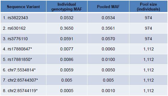Table 3. Five known and three novel variants were identified from large populations and validated by individual genotyping. Individual validation was performed by pyrosequencing (rows 1-3), TaqMan assay (rows 4-6) or Sanger sequencing (rows 7,8). For a broad range of allele frequencies and including five positions with MAF <1%, concordance between pooled sequencing allele frequency estimation and individual genotyping was strong. Positions marked with an asterisk (*) are adapted from previously reported data⁹.

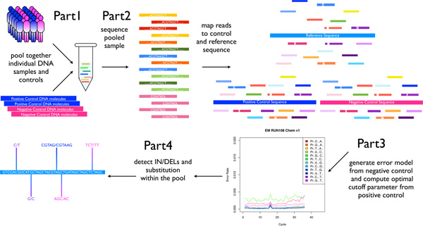Figure 1. Pooled-DNA sequencing and SPLINTER analysis overview. Patient DNA is pooled and amplified at selected loci. The final PCR products are pooled together with a positive and negative control at equimolar ratios. The pooled mix is then sequenced and the resulting reads are mapped back to their reference. Mapped negative control reads are used to generate a run-specific error model. SPLINTER can then be used to detect rare SNPs and indels by incorporating information from the error model and the positive control. [Adapted from Vallania FLM et al, Genome Research 2010] Click here to view larger image.

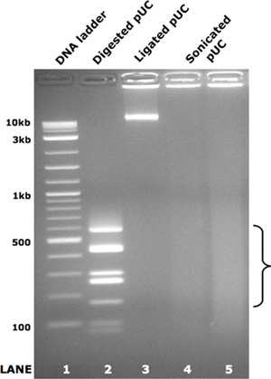Figure 2. Pooled PCR amplicon ligation and sonication. As a demonstration of the ligation and random fragmentation steps in the library preparation protocol, pUC19 vector was enzymatically digested to the fragments shown in lane 2. These fragments were normalized by molecule number, combined and randomly ligated according to step 1.7 above. The resulting large concatamers are shown in lane 3. The ligated concatamers were equally divided and subjected to sonication as described in step 1.8 above. The resulting smear of DNA fragments for each technical replicate are shown in lanes 4 and 5. The bracket highlights the size range used for gel extraction and sequencing library creation.

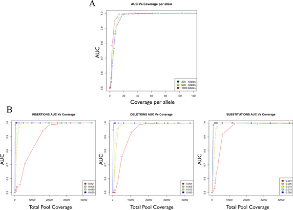Figure 3. Accuracy as a function of coverage for a single allele in a pooled sample. Accuracy is estimated as the Area Under the Curve (AUC) of a Receiver Operator Curve (ROC), which ranges from 0.5 (random) to 1.0 (perfect accuracy). AUC is plotted as a function of coverage per allele for the detection of single mutant alleles in pools of 200, 500 and 1000 alleles (A). AUC is plotted as a function total coverage for substitutions, insertions and deletions (B). [Adapted from Vallania FLM et al, Genome Research 2010].

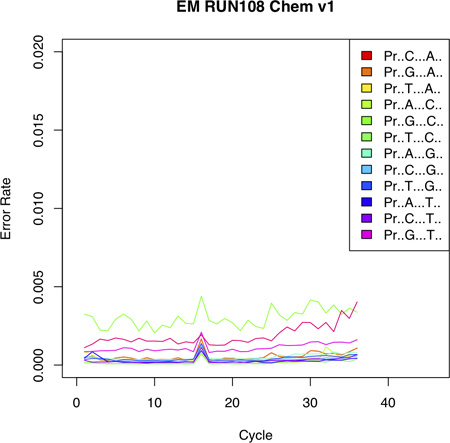Figure 4. Error Plot shows the probability of incorporating an erroneous base at a given position. The error profile shows low error rates with an increasing trend toward the 3' end of the sequencing read. Notably, different reference nucleotides display different error probabilities (see for example probability of incorporating a C given a G as reference). [Adapted from Vallania FLM et al, Genome Research 2010].

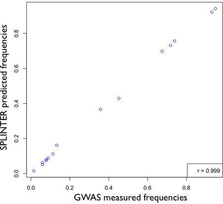Figure 5. Accuracy of SPLINTER in estimating allele frequency for positions that had greater than 25-fold coverage per allele. Based on results in Panel A, Figure 3 showing optimal sensitivity for single variant detection with ≥25-fold coverage, a comparison between pooled-DNA allele frequencies estimated by SPLINTER with allele counts measured by GWAS results in very high correlation (r = 0.999). [Adapted from Vallania FLM et al, Genome Research 2010].

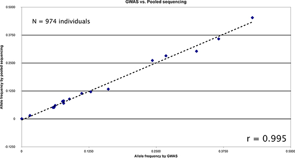Figure 6. Comparison between allele frequencies measured by GWAS compared to SPLINTER estimates from pooled sequencing of 974 individuals. There were 19 common positions between the genotyped loci and the sequence regions for comparison. The resulting correlation is very high (r = 0.99538). Click here to view larger figure.

Discussion

There is increasing evidence that the incidence and therapeutic response of common, complex phenotypes and diseases such as obesity⁸, hypercholesterolemia⁴, hypertension⁷ and others may be moderated by personal profiles of rare variation. Identifying the genes and pathways where these variants aggregate in affected populations will have profound diagnostic and therapeutic implications, but analyzing affected individuals separately can be time and cost prohibitive. Population-based analysis offers a more efficient method for surveying genetic variation at multiple loci.

We present a novel pooled-DNA sequencing protocol paired with the SPLINTER software package designed to identify this type of genetic variation across populations. We demonstrate the accuracy of this method in identifying and quantifying minor alleles within a large pooled population of 947 individuals, including rare variants that were called de novo from the pooled sequencing and validated by individual pyrosequencing. Our strategy mainly differs from other protocols by the incorporation of a positive and a negative control within every experiment. This allows SPLINTER to achieve much higher accuracy and power compared to other approaches¹. The optimal coverage of 25-fold per allele is fixed independently of the size of the pool, making the analysis of large pools feasible as this requirement only scales linearly with the pool size. Our approach is very flexible and can be applied to any phenotype of interest but also to samples that are naturally heterogeneous, such as mixed cell populations and tumor biopsies. Given the ever-increasing interest in pooled sequencing from large target regions such as the exome or genome, our library prep and SPLINTER analysis is compatible with custom-capture and whole-exome sequencing, but the alignment utility in the SPLINTER package was not designed for large references sequences. Therefore, we have successfully utilized the dynamic programming aligner, Novoalign, for genome-wide alignments followed by variant calling from the pooled sample (Ramos et al., submitted). Thus, our pooled sequencing strategy can scale successfully to larger pools with increasing amounts of target sequence.

Disclosures

No conflicts of interest declared.

References

- Vallania FLM, Druley TE, Ramos E, Wang J, Borecki I, Province M, Mitra RD. High-throughput discovery of rare insertions and deletions in large cohorts. Genome Research. 2010;20:1391–1397. doi: 10.1101/gr.109157.110. [DOI] [PMC free article] [PubMed] [Google Scholar]
- Shendure J, Mitra R, Varma C, Church GM. Advanced Sequencing Technologies: Methods and Goals. Nature Reviews of Genetics. 2004;5:335–344. doi: 10.1038/nrg1325. [DOI] [PubMed] [Google Scholar]
- The 1000 Genomes Project Consortium. A map of human genome variation from population-scale sequencing. Nature. 2010;467:1061–1073. doi: 10.1038/nature09534. [DOI] [PMC free article] [PubMed] [Google Scholar]
- Manolio TA, Collins FS, Cox NJ, Goldstein DB, Hindorff LA, Hunter DJ, McCarthy MI, Ramos EM, Cardon LR. Finding the missing heritability of complex diseases. Nature. 2009;461:747–753. doi: 10.1038/nature08494. [DOI] [PMC free article] [PubMed] [Google Scholar]
- Reich DE, Lander ES. On the allelic spectrum of human disease. Trends Genet. 2001;17:502–510. doi: 10.1016/s0168-9525(01)02410-6. [DOI] [PubMed] [Google Scholar]
- Cohen JC, Kiss RS, Pertsemlidis A, Marcel YL, McPherson R, Hobbs HH. Multiple rare alleles contribute to low plasma levels of HDL cholesterol. Science. 2004;305:869–872. doi: 10.1126/science.1099870. [DOI] [PubMed] [Google Scholar]
- Ji W, Foo JN, O'Roak BJ, Zhao H, Larson MG, Simon DB, Newton-Cheh C, State MW, Levy D, Lifton RP. Rare independent mutations in renal salt handling genes contribute to blood pressure variation. Nat. Genet. 2008;40:592–599. doi: 10.1038/ng.118. [DOI] [PMC free article] [PubMed] [Google Scholar]
- Ahituv N, Kavaslar N, Schackwitz W, Ustaszewska A, Martin J, Hebert S, Doelle H, Ersoy B, Kryukov G, Schmidt S. Medical sequencing at the extremes of human body mass. Am. J. Hum. Genet. 2007;80:779–791. doi: 10.1086/513471. [DOI] [PMC free article] [PubMed] [Google Scholar]
- Druley TE, Vallania FL, Wegner DJ, Varley KE, Knowles OL, Bonds JA, Robison SW, Doniger SW, Hamvas A, Cole FS, Fay JC, Mitra RD. Quantification of rare allelic variants from pooled genomic DNA. Nat. Methods. 2009;6:263–265. doi: 10.1038/nmeth.1307. [DOI] [PMC free article] [PubMed] [Google Scholar]
- Mitra RD, Butty V, Shendure J, Housman D, Church GM. Digital Genotyping and Haplotyping with Polymerase Colonies. Proc. Natl. Acad. Sci. 2003;100:5926–5931. doi: 10.1073/pnas.0936399100. [DOI] [PMC free article] [PubMed] [Google Scholar]