Limitations of Constant-Force-Feedback Experiments

Abstract

Single-molecule force spectroscopy has provided important insights into the properties and mechanisms of biological molecules and systems. A common experiment is to measure the force dependence of conformational changes at equilibrium. Here, we demonstrate that the commonly used technique of force feedback has severe limitations when used to evaluate rapid macromolecular conformational transitions. By comparing the force-dependent dynamics of three major classes of macromolecules (DNA, RNA, and protein) using both a constant-force-feedback and a constant-trap-position technique, we demonstrate a problem in force-feedback experiments. The finite response time of the instrument’s force feedback can modify the behavior of the molecule, leading to errors in the reported parameters, such as the rate constants and the distance to the transition state, for the conformational transitions. We elucidate the causes of this problem and provide a simple test to identify and evaluate the magnitude of the effect. We recommend avoiding the use of constant force feedback as a method to study rapid conformational changes in macromolecules.

Introduction

In recent years, the application of single-molecule force spectroscopy to the study of biological molecules has provided insights that would be unobtainable by other methods. Studies ranging from the initial work on kinesin (6) and myosin (7) to investigations of polymerases (8) and the more-complicated ring ATPases (9) have improved our understanding of the properties and mechanisms of a variety of systems under force, such as DNA structure (1,2), RNA folding (3), protein folding (4,5), and various molecular motors.

A typical experiment follows the trajectory of a single molecule in time, allowing for the observation of transient or rare events that would otherwise be masked when observing the average properties of a large number of molecules in ensemble experiments. Applying force to the molecule perturbs the energetics of the system, influencing whether and to what extent conformational changes will occur (10). Finally, the reaction is observed along a well-defined order parameter, the end-to-end distance of the molecule, that may serve as a good reaction coordinate. Under certain conditions, one can infer landmarks along this reaction coordinate, such as the distance to the transition state, by measuring the lifetimes (or rate constants) of conformational states as a function of force, allowing for a detailed mapping of the energy landscape.

The force dependence of these rate constants can be described using a modified Bell’s relationship (11,12)

$$k\left(F\right)=k_m{k}_0\exp \left(\frac{F\Delta x^{‡}-\frac{1}{2}\kappa \Delta x^{‡2}}{k_{\text{B}}T}\right),$$ (1)

where, for an optical trap experiment, k_m represents the contribution of experimental parameters such as the bead size, trap stiffness, and handle length to the observed rate constant; k₀ is the intrinsic rate constant of the molecule in the absence of force; F is the applied force; Δx^‡ is the distance to the transition state; κ is the spring constant of the system; k_B is the Boltzmann constant; and T is the absolute temperature (see Supporting Material). In this notation, the applied force and effective spring constant of the system are positive, and the distance to the transition state is positive from the folded state to the unfolded state and negative from the unfolded state to the folded state. Although formally Δx^‡ is a function of force, experimentally over small force ranges (∼1 pN), Δx^‡ is observed to be constant. From this simple relationship, the distances to the transition-state barriers (Δx^‡) are fully determined from the folding and unfolding rates as a function of force.

Determining the distances to the transition state from single-molecule experiments requires accurate measurements and analyses to extract the lifetimes of the individual states. The mode of force control (constant-force-feedback, constant-trap-position, or constant loading rate) and other parameters, such as the trap stiffness, bead size, tether length, and viscosity, can influence both the behavior and the observed measurements of the molecule. In addition, the analyses can be complicated by factors such as noise, limited sampling frequency, and missed transitions. Therefore, investigators have developed several different strategies to identify the states and determine the associated lifetimes or rate constants (13–17). Previous studies evaluating the equilibrium behavior of an RNA hairpin using both constant-force-feedback and constant-trap position data did not report on any differences between these two experiments (18,19). Our evaluation of these studies, however, reveals a significant error in the constant-force-feedback results, and suggests that this is a general problem for other constant-force-feedback experiments.

Here, we revisit the effect of the constant-force-feedback methods on the measurement of conformational lifetimes. Using data from DNA, RNA, and protein systems in which the molecules fold and unfold under either a constant-force-feedback or constant-trap-position experiment, we identify an unreported error arising from the feedback, which directly affects and thereby alters the behavior of the molecule. This change in behavior of the molecule contributes to missed short-lived dwell times. We demonstrate that this results in errors in the reported kinetic parameters, such as the rate constants as a function of force, and the calculated distance to the transition state, because they do not describe the true force-dependent behavior of the molecule of interest. Finally, given these limitations, we recommend that constant-trap-position experiments should be used in place of constant-force-feedback experiments for collecting single-molecule force spectroscopy data on molecules undergoing rapid conformational changes.

Materials and Methods

Preparation of single-molecule constructs

The p5ab RNA hairpin from Tetrahymena thermophilia was provided by Jin Der Wen and Ignacio Tinoco, and prepared as described previously (18). The DNA hairpin data were provided by Nuria Forns and Felix Ritort (20). The wild-type sperm whale myoglobin gene was provided by D. Barrick, and the H36Q mutant of apomyoglobin was prepared as previously described (21).

Instrumentation

The data were collected using a dual-beam counterpropagating optical trap. A piezo actuator controlled the position of the trap and allowed position resolution to within 0.5 nm with drift of <1 nm/min (22). When operating in constant-force-feedback mode, the feedback controls the position of the trap and hence the force on the bead and molecule, with a frequency of 2 kHz and a step size proportional to 10% of the force difference between the two states. An average force could be maintained within 0.01 pN of the set value with a standard deviation of 0.1 pN at 100 Hz. Data were collected at 4 kHz and averaged down to 1 kHz before they were written to disk. Due to hardware constraints from the limited throughput of a USB 1.0 connection, ∼40% of the data points at 4 kHz were dropped. Therefore, the data at 1 kHz varied from an average of one to four data points collected at 4 kHz, and consequently ∼2% of the data at 1 kHz were not reported. Because of the limited response time of the feedback, the data were analyzed at a lower frequency (100 Hz). At this frequency, the missed data at 1000 Hz due to the limitations of the hardware did not affect the average force. All constant-force experiments and the constant-trap-position experiments for the DNA hairpin were collected at this sampling frequency. For the constant-trap-position experiments on the RNA and protein systems, we recorded higher-frequency data at 50 kHz by bypassing the limiting hardware and recording the voltage corresponding to the force on the tether directly from the position-sensitive detectors.

Equilibrium force spectroscopy experiments

Equilibrium single-molecule force spectroscopy experiments were carried out using the optical trap described above. In this setup, a single molecule is tethered between two polystyrene beads: a pipette tip holds a 2.1 μm diameter bead in place by suction, and a counterpropagating dual beam optical trap holds a second, 3.2 μm diameter bead (see Fig. 1). By monitoring the bead displacement within the trap, one can determine both the force and the relative extension of the tether (23). The molecule of interest (DNA, RNA, or protein) is attached to the beads through functionalized double-strand DNA (dsDNA; referred to as dsDNA handles). These dsDNA handles provide space between the bead surfaces and the molecule, preventing any nonspecific interactions with or between the beads from influencing the behavior of the molecule. The dsDNA handles are attached to the target molecule at specific sites to determine the axis along which the force is applied (4,24). The effective spring constants were 0.03 ± 0.01 pN/nm, 0.06 ± 0.01 pN/nm, and 0.03 ± 0.01 pN/nm for the DNA, RNA, and protein molecules, respectively.

Figure 1.

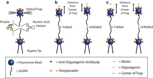
Optical trap experimental design. (a) Geometry of experiments depicting bead attachment via dsDNA handles to the macromolecule of interest. (b) In a constant-force-feedback experiment, the average bead distance from the trap center (i.e., the average force) is maintained constant by the force feedback controlling the position of the optical trap. (c) In a constant-trap-position experiment, the trap position is constant, and as the molecule folds or unfolds, the bead distance from the trap center changes, resulting in a change in the force on the bead.

We carried out constant-force-feedback and constant-trap-position experiments on three types of macromolecules (all of which were previously studied by the optical trap method): a DNA hairpin (20), p5ab RNA hairpin (3,18), and protein sperm whale apomyoglobin at pH 5 (21). We monitored different observables in each experiment (trap position for the constant-force-feedback experiments, and force for the constant-trap-position experiments) to follow the trajectory of a single molecule.

For each experiment, the behavior of the single molecule was observed for 60 s at a given force or trap position, during which time many folding and unfolding events were observed (Fig. 2). For each molecule, the behavior was observed at five or more different forces or trap positions. These experiments were repeated on five or more different molecules.

Figure 2.

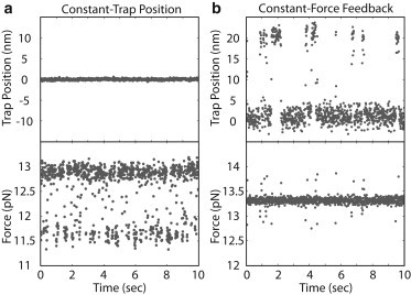
Constant-trap-position and constant-force-feedback experimental data. (a) Trap position and force versus time for a constant-trap-position experiment. (b) Trap position and force versus time for a constant-force-feedback experiment. Data averaged down to 100 Hz.

Constant-force-feedback experiments

During the constant-force-feedback experiments, when the molecule folds (unfolds), the fiber becomes shorter (longer) and the force on the molecule increases (decreases). The feedback responds to this change by moving the position of the trap to maintain the force on the bead constant to a preset value. This change in trap position reflects the conformation of the molecule as defined by its end-to-end extension. Force feedback is fundamentally limited primarily by the relaxation time of the mechanical component that controls the position of the trap (22). After the trap has been moved, the feedback has to wait several relaxation times before the components become stable, before a second reading can be taken to implement another step in the feedback loop. Further, the feedback has to go through several loops to move the trap position fully between the two states (in the case of these experiments, 20 nm, the approximate distance between the folded and unfolded state for the molecules studied here). In this setup, the response time of the force feedback of the instrument limits the timescale at which the force is constant and at which the force and trap position are analyzed to 100 Hz.

Constant-trap-position experiments

In the constant-trap-position experiments, when the molecule undergoes a folding (unfolding) transition, the force increases (decreases), and therefore the force measurements are used to infer the state of the molecule indirectly. In this setup, the time resolution is greater than in a constant-force-feedback experiment and is determined by the response time of the bead in the trap rather than the response time of the feedback. We determined the response time experimentally by measuring the power spectrum of the force on the bead and determining the corner frequency of the system (25). In our experiments, the corner frequency ranged between 1 kHz to 2.5 kHz.

Data analysis

For all of the constant-force-feedback experiments, the data were averaged down to 100 Hz before analysis. For the constant-trap-position experiments, the data were averaged down to 100 Hz (for direct comparison with the constant-force-feedback experiments) or subsampled down to 1000 Hz (for analysis with the Bayesian hidden Markov model (BHMM) before analysis. Relative force precision for measurements on a single trapped molecule were very good (i.e. repeated measurements of ln(k) as a function of force were highly reproducible). However, the force precision between molecules was ± 0.5 pN and therefore each molecule was analyzed separately.

To determine the kinetic parameters for the system, we identified each state and determined its respective lifetimes at a given force using one of two different approaches. The first is a simple partition method similar to those used in previous studies (3,4,18), and was used for the 100 Hz data to allow a more direct comparison with previously published results as well as between the constant-trap and constant-force-feedback experiments. Although this method is simple and direct, it requires clear resolution between the signals of each state. Poor separation between the two states results in an overestimate of the number of transitions and a corresponding underestimate of the average lifetime of the state (and hence an overestimate of the rate constants for leaving the state). For data with a lower signal/noise ratio, a second, more sophisticated approach, such as a BHMM approach, is needed (26). For the data averaged to 100 Hz, the partition method was sufficient given the resolution between the two states. However, constant-trap-position experiments subsampled to 1000 Hz had a lower signal/noise ratio and thus required the BHMM method. Application of the BHMM method to all of the constant-force data was not feasible because of the inherent drift in the data. A comparative study on a control set of data (constant-force data with low drift) showed equivalent results with each approach.

Partition method

Using a histogram of the constant-force data with a bin size of 0.5 nm, we set a partition to the minimum between the two Gaussian peaks. A transition was detected when the signal crossed this partition, defining the beginning or end of the lifetime of the state. At the measured average force, the inverse of the average lifetime (i.e., the rate constant) is the maximum-likelihood estimate for fitting the observed lifetime distribution with an exponential.

BHMM

We analyzed the constant-trap-position experiments using a BHMM approach (27–30). This Bayesian extension of the standard machine learning approach of hidden Markov model (HMM) analysis (31) allows one to quantify the experimental uncertainties directly by sampling from the posterior of the model parameters (transition probabilities and Gaussian state observable distributions) given the data, rather than by simply identifying the maximum-likelihood model parameters as in the traditional HMM approach. To that end, we augment the standard HMM likelihood function with a prior that enforces the physical detailed balance constraint in the transition matrix. Sampling from the posterior proceeds by a Gibbs sampling approach, alternating updates of the reversible transition matrix (32,33), the hidden state sequence, and the Gaussian state observable distributions using standard techniques (27–30).

The BHMM code we used here sampled two-state models over the measurement histories of force at constant-trap positions, producing estimates of the average force that characterize each state and the transition probabilities among the states, as well as confidence intervals (CIs) that characterize the uncertainty in these values due to finite-sample statistics. After subsampling the force data to 1000 Hz to produce Markovian statistics (verified by examination of force-autocorrelation functions), the method samples models consistent with the data using a Gibbs sampling strategy that assumes the force measurements from each state (including measurement error) are normally distributed about the average force for that state. Here, the number of states was fixed to two after the two-state nature of the data was verified by inspection of the force traces. The first 50 BHMM samples after starting from the maximum-likelihood estimate were discarded, and 1000 samples were subsequently generated to collect statistics on average forces and transition probabilities, as well as to generate the 95% CIs reported here. Matrices of rate constants K were computed from transition matrices T(τ) using the standard relationship T(τ) = exp[K(τ)] through the use of the matrix logarithm, where K is the 2 × 2 matrix of rate constants k_ij, and τ is the observation time.

The MATLAB (The MathWorks, Natick, MA) code used for the BHMM approach has been deposited and is freely obtained from http://simtk.org/home/bhmm/. Complete implementation and validation details of this code are described elsewhere (26).

Determination of the distance to the transition state and the coincident rate constants

For a given state, a linear fit of the natural logarithm of the rate constants at each average force determined the distance to the transition state according to the modified Bell’s model (Fig. 3). The crossing point between the two linear fits determined the coincident rate constant (i.e., the rate constant at which the folding and unfolding rate constants are equal). All reported fits had R² values > 0.9. The fit values reported were the average of at least five different fibers each analyzed separately and with data collected from five to 25 different average forces.

Figure 3.

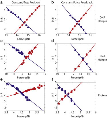
Linear fits of the natural log of the rate constant (ln k) versus force. (a and b) Fits of the constant-trap-position and constant-force-feedback data for the DNA hairpin. (c and d) Fits of the constant-trap-position and constant-force-feedback data for the RNA hairpin. (e and f) Fits of the constant-trap-position and constant-force-feedback data for the protein system.

Simulation

A simple simulation modeling the molecule’s behavior under constant-force feedback was run at 10 kHz and assumed that the bead responded instantaneously to a change in the force. At each time step, we calculated the probability of a folding/unfolding transition at the instantaneous force using the kinetic parameters measured from the constant-trap-position experiments. Lifetimes were drawn from an exponential distribution determined by the kinetic parameters, and a random number generator determined whether a folding or unfolding event occurred, modeling the stochastic nature of the events. The feedback controlled the position of the trap, and therefore the force on the bead and molecule, with a frequency of 2 kHz and a step size proportional to 10% of the force difference between the two states. For each set of conditions, five simulated experiments were averaged down to 100 Hz, analyzed using the partition method, and fit with the modified Bell’s model. The initial effective spring constant was set to 0.1 pN/nm for the nucleic acid system and 0.05 pN/nm for the protein system. The initial rate constants and the effective spring constants were varied between sets of simulations to test the effect of these parameters on the simulated experiment. Because the purpose of this simulation was to probe the role of the changing potential in missed transitions, the simulation neglected any changes in the signal/noise ratio and the intrinsic rate constants as a function of the effective spring constant of the system.

Results

Constant-force-feedback experiments

Constant-force-feedback experiments on all three systems (DNA, RNA, and protein) revealed many folding and unfolding events for each single-molecule tether (Fig. 2) and were repeated on multiple molecules. These experiments revealed apparent two-state kinetics and extension changes (Δx_total (measured)) consistent with predictions based on calculations given the native structure and a worm-like chain model for the unfolded state (4,34,35) and previously reported results for each of the molecules (3,18,20,21).

We analyzed each molecular tether separately to determine kinetic parameters, such as the rate constant, as a function of the average force (see Materials and Methods). Using the modified Bell’s model, we then determined the coincident rate constants and the distance to the transition state (Table 1 and Fig. 3). For all three systems, the sum of the distances to the transition state (Δx^‡_Folding + Δx^‡_Unfolding) was inconsistent and significantly larger than the directly measured change in extension (Δx_total (measured); Table 1). The sum of the calculated distances overestimated the total measured extension change between the two states by an average of 34% for both nucleic acid hairpins and 97% for the protein.

Table 1.

Results from the linear fits of the ln k versus force for constant-force-feedback and constant-trap-position experiments

Molecule	Δx‡Unfolding (nm)∗	Δx‡Folding (nm)∗	ΔxTotal (sum) (nm)∗	ΔxTotal (measured) (nm)†	Ratio of ΔxTotal‡	ln(kCoincident)∗
Constant-force feedback (partition method, 100 Hz)
DNA hairpin	11.3 ± 0.6	12.1 ± 1.1	23.5 ± 1.6	17.7 ± 0.4	1.33	1.3 ± 0.4
RNA hairpin	12.1 ± 2.5	13.9 ± 2.6	26.0 ± 3.2	19.2 ± 0.4	1.35	0.9 ± 0.4
Protein	14.8 ± 8.1	22.4 ± 6.4	37.2 ± 5.6	18.9 ± 0.4	1.97	2.0 ± 0.6
Constant-trap position (partition method, 100 Hz)
DNA hairpin	9.3 ± 1.4	10.9 ± 1.8	20.2 ± 1.5	17.7 ± 0.4	1.14	1.3 ± 0.6
RNA hairpin	8.9 ± 5.6	13.2 ± 3.6	22.1 ± 6.6	19.2 ± 0.4	1.15	0.9 ± 0.9
Protein	7.5 ± 3.1	15.9 ± 5.1	23.4 ± 6.0	18.9 ± 0.4	1.24	2.4 ± 0.7
Constant-trap position (BHMM method, 1000 Hz)
DNA hairpin	7.8 ± 0.7	10.2 ± 0.9	18.0 ± 1.3	17.7 ± 0.4	1.02	1.7 ± 0.5
RNA hairpin	7.9 ± 1.9	11.6 ± 2.1	19.5 ± 3.1	19.2 ± 0.4	1.02	1.5 ± 0.7
Protein	6.1 ± 1.1	14.4 ± 3.9	20.5 ± 3.2	18.9 ± 0.4	1.09	2.8 ± 0.7

^∗Average values reported with a 95% CI.

^†Distance determined from fitting a histogram of the trap position from a constant-force-feedback experiment with two Gaussian distributions and determining the difference between the two Gaussian means with a 95% CI.

^‡Ratio of the calculated sum of the distances to the transition state to the experimentally measured distance between the two states.

Constant-trap-position experiments

The constant-trap-position experiments also revealed apparent two-state kinetics for each of the three molecules and similar extension changes (determined from the change in average force between the two states; Fig. 2). However, unlike the constant-force-feedback experiments, the sums of the distances to the transition state (Δx^‡_Folding + Δx^‡_Unfolding) were more consistent with the total measured extension changes. Analysis of the data at 1000 Hz using the BHMM method produced only slight overestimates of 2% for both nucleic acid hairpins and 9% for the protein, but well within the error of the measurements (Table 1). To make a direct comparison with the constant-force-feedback experiments, we averaged these data down to 100 Hz and evaluated them using the same partition method used to analyze the constant-force-feedback experiments. The resulting distances were closer to the measured distances but overestimated the measured extension change by 14%, 15%, and 24% for the DNA, RNA, and protein molecules, respectively. Thus, independently of the sampling frequency, the constant-trap-position data yielded distances more consistent with the observed extension changes.

In both experimental configurations, the resulting rate constants as a function of force were fit using the modified Bell’s model (Fig. 3) without any detectable nonlinearity or change in the distance between the folded and unfolded states over this narrow force range (∼1 pN). Therefore, more detailed models that account for changes in the end-to-end extension of the molecule and the corresponding changes of the distances to the transition state with force (i.e., changes in the slope of ln k versus force) were not warranted and would not have provided additional insight (36). The distances to the transition state and the rate constant at which the forward and reverse rate constants are equal (the coincident rate constant (k_c)) are shown in Table 1. Results from the analyses of each individual molecule are shown in Table S1.

The resulting kinetic parameters depend on the type of experiment conducted and the frequency at which the data were analyzed (see Table 1). The coincident rate constants from the constant-force-feedback experiments are equal to or less than those obtained with constant-trap-position experiments. This trend is the opposite of what would be expected when considering the effect of the spring constants on the system, because the constant-trap position experiments (κ > 0) should have lower rate constants than the constant-force-feedback experiments (κ = 0; see Supporting Material). The magnitude of this discrepancy varies depending on the molecule. A comparison of the constant-force-feedback experiments analyzed at 100 Hz and the constant-trap-position experiments analyzed at 1000 Hz shows differences in the coincident rate constants for the DNA and RNA hairpin of 1.8 s⁻¹ and 2 s⁻¹, respectively, whereas for the protein apomyoglobin, the difference in the rate constant is 9 s⁻¹.

Discussion

For all three experimental systems studied (DNA, RNA, and protein), the distances to the transition state should be the same regardless of the experimental method used. The sum of the two distances to the transition state should be the same and consistent with the independently measured extension change of the molecule. Any discrepancy in these values indicates an error in the determined kinetic parameters. In addition, the rate constants measured by the constant-force-feedback experiment should be greater than those measured by the constant-trap-position experiment, due to the contribution of the effective spring constant to the force-dependent barrier height (see Supporting Material).

Although the deviation between the values obtained depends on both the experimental mode and the specific molecule measured, there are consistent trends in the distances to the transition state and the coincident rate constants. A comparison of the 100 Hz data analyzed with the partition method reveals that the distances for the constant-force-feedback experiments have significantly greater error than those determined by the constant-trap-position experiments. Analyzing the constant-trap-position data at a higher frequency (1000 Hz) further reduces the error and produces distances consistent with the expected values. The coincident rate constants also show a clear trend, with constant-trap-position experiments measuring rate constants that are greater than or equal to the constant-force-feedback experiments, in direct contrast to expectations. In addition, for a given experimental method, the error (as shown as the ratio of Δx_Total in Table 1) in the sum of the distances to the transition state are always greater for the protein than for the nucleic acid hairpins.

Only two parameters—the frequency at which the data were analyzed and the force feedback—could contribute to the differences between the experiments, because all other experimental variables (e.g., the molecular sample, trap stiffness, bead size, and handle length) were the same. The discrepancy is not a result of the analysis method either, because both the partition and BHMM methods yielded similar results when used to analyze the same constant-force-feedback data set at 100 Hz (see Materials and Methods).

One potential explanation for the discrepancies is missed transitions. The issue of missed transitions for single-molecule systems due to limited sampling bandwidth is not new, and a variety of methods have been developed to deal with these kinds of data (13–15). In our experiment, a missed set of transitions (to and from one state) had two effects on the calculated average lifetime or rate constant: an underestimate of the number of events (N) and an overestimate of the sum of the lifetimes (Σt_i). Both result in an overestimate of the lifetime of the state. Indeed, the comparison of the constant-trap-position date analyzed at 100 Hz and 1000 Hz clearly demonstrates this affect. However, this cannot account for all of the discrepancies. A comparison between the constant-force-feedback and constant-trap-position data obtained at the same frequency (100 Hz) reveals disagreement between the two experiments, indicating that the error is not solely the result of the limited sampling frequency. The force feedback must be causing additional error in the measurements.

Due to the finite-time limitations of the force feedback, the system can only maintain an average constant force on a timescale greater than the timescale of the feedback (10 ms for these experiments). Force fluctuations that occur at shorter timescales could significantly modify the behavior of the molecule and lead to inaccurate results in the force-feedback mode. To illustrate this point, consider a molecule in the unfolded state. When the molecule folds, the tether becomes shorter and the bead in the trap moves, resulting in a transient increase in the force. During this transient high force, the unfolding rate constant (Eq. 1) increases, which in turn increases the likelihood of the molecule unfolding (i.e., the rate constant) before the feedback has a chance to alter the position of the trap, resulting in a transition to and from the folded state that is missed (illustrated in Fig. 4 a). During an experiment, transitions are therefore missed when the molecule populates a given state for a time shorter than the response timescale of the system. Because the finite response time of the feedback changes the potential, which in turn changes the rate constants, the missed transitions cannot be treated by the simpler analysis methods that assume constant rate constants and have been use to address other types of missed transitions, such as those due to sampling rate limitations (13–15).

Figure 4.

Illustration of a hypothetical missed transition and its effect on the measured rate constants and distances to the transition state. (a) Illustration of a missed transition during a constant-force-feedback experiment, showing the true (blue) and measured (red) behaviors of the molecule. (b) The ln k versus force for the actual (blue) and measured (red) behaviors of the molecule during a constant-force-feedback experiment. (c and d) The distributions of long (c) and short (d) lifetimes are shown for two different states, with the average lifetime marked by the red bar. The difference in the average lifetimes between c and d represents the change that would occur for a system with a total distance between the two states of 20 nm and an effective spring constant of 0.1 pN/nm. The black (c) and striped (d) regions indicate the number of missed transitions given a force-feedback limit of 10 ms, as in the constant-force-feedback experiments.

The measured behavior is very similar to what is observed with a limited sampling rate. For example, when a short transition is missed, it results in an erroneous observation of a long lifetime (biasing the results to a longer average lifetime or lower rate constant) and similarly results in the erroneous absence of a short lifetime in the other state (similarly biasing toward a longer average lifetime or lower rate constant). Therefore, a missed transition increases the measured lifetime of both states; however, the effect is more pronounced in the longer-lived state. The magnitude of the difference between the actual lifetime and the measured lifetime is a function of the number of missed transitions. This difference becomes larger at more extreme forces when more transitions are missed to and from the short-lived state relative to the long-lived state. As a consequence, the measured change in the rate constants as a function of force (proportional to the distance to the transition state) is also a function of the number of missed transitions and results in an overestimate of the distance to the transition state (Table 1 and Fig. 4 b).

The trends in the data are consistent with this changing potential and missed transition hypothesis. For each system, the measured hopping rates are equal to or lower in the constant-force-feedback experiments than in the constant-trap-position experiments. The distances to the transition state are larger in the constant-force-feedback experiments than in the constant-trap-position experiments, and, as previously mentioned, the sums of these distances in the constant-force-feedback experiments are inconsistent with the independently determined distance between the equilibrium states of the system. This hypothesis also predicts that the greater the coincident rate constant (measured by the constant-trap-position experiments at 1000 Hz), the larger will be the error in the distances to the transition state as measured by the constant-force-feedback experiments. A system with a greater coincident rate constant would, on average, have shorter lifetimes in both states when compared with a slower system. The shorter lifetimes result in more missed transitions and a larger error in the distance to the transition state. Both the DNA and RNA models have similar coincident rate constants measured from a constant-trap-position experiment, and consequently have the same magnitude of discrepancy (∼34%) in the total distance change. The protein has the largest coincident rate constant (i.e., the fastest hopping rate and thus the greatest number of missed transitions) and shows the largest distance error, with a difference of 97%.

To better illustrate the discrepancies between the constant-force-feedback and constant-trap-position experiments, we ran a simple simulation. We evaluated two models, one representative of the DNA and RNA systems and the other representative of the protein system, using kinetic parameters (e.g., the distance to the transition state and the intrinsic rate constants as a function of force) based on those measured by the constant-trap-position experiments. We simulated constant-force-feedback experiments using instrumental parameters such as the frequency and amplitude of the force feedback. We then analyzed the simulated data using the partition method in the same manner employed for the experimental data. With these simulations, we modeled the changing potential on the system and the effect of the force-feedback and other experimental parameters, such as the intrinsic rate constants of the molecule (i.e., how fast the molecule hops) and the effective spring constant of the system (1/κ_eff = 1/κ_trap + 1/κ_tether), on the measured kinetic parameters. The results of the various simulations are shown for the nucleic acid hairpin model and the protein model in Table 2.

Table 2.

Results from the linear fits of the constant-force-feedback simulated data

Molecule	Effective spring constant (pN/nm)	Relative rate constant∗	Δx‡Unfolding (nm) †	Δx‡Folding (nm) †	ΔxTotal (sum) (nm) †	Ratio of calculated to expected ΔxTotal‡	ln(kCoincident)
Nucleic acid hairpin
Initial parameters			7.9	11.6	19.5	1	1.5
	0.1	0.25 ki	12.4 ± 0.7	12.2 ± 0.5	24.6 ± 0.9	1.26	−0.1
	0.1	0.5 ki	13.9 ± 0.9	12.3 ± 0.6	26.2 ± 1.1	1.34	0.4
	0.1	1 ki	16.0 ± 1.4	15.3 ± 0.8	31.3 ± 1.6	1.61	0.8
	0.1	2 ki	27.2 ± 2.8	14.7 ± 1.5	41.9 ± 3.2	2.15	1.0
	0.1	4 ki	32.4 ± 3.1	24.3 ± 2.1	56.7 ± 3.7	2.91	0.9
	0.05	1 ki	9.9 ± 0.5	11.9 ± 0.3	21.8 ± 0.6	1.12	1.3
	0.075	1 ki	11.5 ± 0.7	12.5 ± 0.3	24.0 ± 0.8	1.23	1.2
	0.1	1 ki	16.0 ± 1.4	15.3 ± 0.8	31.3 ± 1.6	1.61	0.8
	0.125	1 ki	28.6 ± 3.4	20.3± 1.6	48.9 ± 3.8	2.51	0.1
	0.5	1 ki	45.1 ± 10.3	22.0 ± 2.6	67.1 ± 10.6	3.44	−1.4
Protein
Initial parameters			6.1	14.4	20.5	1	3.0
	0.05	0.25 ki	11.1 ± 1.2	14.8 ± 0.4	25.9 ± 1.3	1.26	1.3
	0.05	0.5 ki	12.0 ± 1.2	15.2 ± 0.3	27.2 ± 1.2	1.33	1.9
	0.05	1 ki	22.7 ± 3.3	15.5 ± 0.6	38.2 ± 3.4	1.86	2.2
	0.05	2 ki	28.1 ± 1.0	16.9 ± 1.6	45.0 ± 1.9	2.20	2.4
	0.05	4 ki	29.0 ± 3.1	21.2 ± 0.7	50.2 ± 3.2	2.45	2.8
	0.01	1 ki	7.7 ± 0.5	13.5 ± 0.4	21.2 ± 0.6	1.03	2.8
	0.025	1 ki	9.9 ± 0.8	14.3 ± 0.3	24.2 ± 0.6	1.18	2.7
	0.05	1 ki	22.7 ± 3.3	15.5 ± 0.6	38.2 ± 3.4	1.86	2.2
	0.75	1 ki	32.2 ± 3.6	17.0 ± 1.0	49.2 ± 3.7	2.40	1.7
	0.1	1 ki	39.9 ± 6.0	22.7 ± 2.2	62.6 ± 6.4	3.05	0.1

^∗Relative rate constants are reported as a multiple of k_i, the intrinsic rate constants, measured from the constant-trap-position experiments.

^†Average values reported with a 95% CI.

^‡Ratio of the calculated sum of the distances to the transition state to the expected sum of the distances to the transition states set in the initial parameters.

The simulations support the conclusion that the discrepancy between the constant-force-feedback and constant-trap-position experiments is primarily a product of missed transitions, and the magnitude of the discrepancy is proportional to the number of missed transitions. The simulations of both types of molecules (nucleic acid hairpins and protein) under similar experimental conditions resulted in distances to the transition state similar to those obtained in the corresponding constant-force-feedback experiments, validating the simulation (Table 2). Changes in the simulation parameters for the system (i.e., the intrinsic rate constants or the effective spring constant of the system) changed the measured kinetic parameters. For example, decreasing the intrinsic rate constants resulted in longer lifetimes and fewer missed transitions, and consequently the measured coincident rate constants and distances to the transition state were closer to the true values. Increasing the initial intrinsic rate constants resulted in more missed transitions and larger deviations in the measured kinetic parameters. A larger effective spring constant resulted in a larger change in the force and consequently a larger change in the lifetime of the state. This resulted in more missed transitions and hence a larger deviation between the calculated and true rate constants and distances to the transition state (illustrated in Fig. 4 b).

These issues, of course, depend very much on the relative timescales of the molecular transitions and the feedback. One can determine the validity of a constant-trap or constant-force-feedback experiment by comparing the sum of the distances to the transition state with the measured extension change of the molecule. If the values are commensurate, then the number of missed transitions is negligible. In addition, for a given force, a lower limit of the number of missed transitions can be estimated assuming the response time is instantaneous after a delay time of τ_f, as illustrated in Fig. 4, c and d. The fraction of missed transition (f_m) can be estimated by

$$f_m=1-\exp \left[-{\tau }_f{k}_A\exp \left(\frac{\Delta F_{A-B}·\Delta x^{‡}}{k_{\text{B}}T}\right)\right],$$ (2)

where k_A is the rate constant in state A, ΔF is the change in force between the two states, Δx^‡ is the distance to the transition state, k_B is the Boltzmann constant, T is the absolute temperature, and τ_f is the response time of the system, limited by either the corner frequency of the system or the response time of the feedback. Using the parameters from the constant-trap-position experiment, one can estimate the number of missed transitions at a given force for the constant-force-feedback experiments. In addition, this relationship can be used to estimate the number of missed transitions from a constant-force-feedback experiment as a further check on the validity of the experiments. This relationship, however, cannot be used to correct for missed transitions without prior knowledge of the true kinetic parameters.

In the constant-trap-position experiments, the effective spring constant of the system influences the results, and this raises the question as to what effective spring constant should be chosen for a given experiment. Compared with a true constant-force experiment (or passive force clamp with κ ∼ 0 pN/nm) (12), a positive spring constant provides several advantages in terms of the experimental design. First, the response time of the bead is determined by the spring constant of the system: the stiffer the trap, the faster is the response time of the bead (i.e., the corner frequency is higher), which enables a faster sampling time for a system with a positive spring constant (25). Second, the average lifetime of a state increases, as discussed in the Supporting Material. These two factors (i.e., a higher sampling frequency and longer average lifetimes) decrease the likelihood of missing transitions. Third, a higher stiffness increases the force signal/noise ratio and, if a dual-trap geometry is used, the observation of both beads results in a higher signal/noise ratio (37). In addition, for slower systems in which missed transitions are not a concern, de Messieres et al. (38) showed that a polymer constrained by a positive spring constant allows equilibrium behavior to be measured more efficiently. A more practical consideration is that a true constant-force experiment requires a second detection laser because there is no change in the force on the trapped bead and therefore no detectable change in the signal of the trapping bead, increasing the complexity and cost of the instrument (12).

In sum, a higher positive spring constant will increase the sampling frequency, the lifetimes of the states as a function of average force, and the force signal/noise ratio, and thus provide the greatest resolution (in both time and force) and the highest-quality data. If the effective spring constant is too stiff, the large force change between the two states will result in a system that may not hop under the experimental observation time. Therefore, although a positive spring constant is desirable, an excessively stiff spring constant will impose additional constraints.

We conclude that the constant-trap-position experiment with sampling frequency limited only by the response time of the bead is the better experiment for measuring state lifetimes and determining distances to the transition state using the modified Bell’s model. Force feedback will always have a slower response time than a constant-trap-position experiment because of the delay time caused by the feedback loop and relaxation time of the mechanical components of the system. Force fluctuations below this frequency can affect the kinetics of the system. Further, because of these force fluctuations, the molecule is not held at a constant force with the feedback creating a changing potential on the system. Thus, the analysis of the data at a constant force is not valid.

Conclusions

In summary, we have identified an error arising from force fluctuations and missed transitions during constant-force-feedback experiments on systems that hop between two or more states. This study demonstrates that the constant-force-feedback experiments for all the systems studied here result in an underestimate of the rate constants and an overestimate of the distances to the transition state. We conclude that a constant-trap-position experiment with a constant potential and a sampling frequency limited only by the response time of the trapped bead is superior to a feedback experiment for measuring state lifetimes and determining distances to the transition state for macromolecules that undergo rapid conformational changes. Regardless of the particular experiment used (i.e., constant-force feedback or constant-trap position), if the system has lifetimes that are shorter than the response time of the bead, transitions will be missed, potentially resulting in errors in the measured kinetic parameters. This point emphasizes the importance of confirming that the sum of the distances to the transition state equals the independently determined distance between the equilibrium states of the system.

References

- 1.Smith S.B., Finzi L., Bustamante C. Direct mechanical measurements of the elasticity of single DNA molecules by using magnetic beads. Science. 1992;258:1122–1126. doi: 10.1126/science.1439819. [DOI] [PubMed] [Google Scholar]
- 2.Smith S.B., Cui Y., Bustamante C. Overstretching B-DNA: the elastic response of individual double-stranded and single-stranded DNA molecules. Science. 1996;271:795–799. doi: 10.1126/science.271.5250.795. [DOI] [PubMed] [Google Scholar]
- 3.Liphardt J., Onoa B., Bustamante C. Reversible unfolding of single RNA molecules by mechanical force. Science. 2001;292:733–737. doi: 10.1126/science.1058498. [DOI] [PubMed] [Google Scholar]
- 4.Cecconi C., Shank E.A., Marqusee S. Direct observation of the three-state folding of a single protein molecule. Science. 2005;309:2057–2060. doi: 10.1126/science.1116702. [DOI] [PubMed] [Google Scholar]
- 5.Gebhardt J.C., Bornschlögl T., Rief M. Full distance-resolved folding energy landscape of one single protein molecule. Proc. Natl. Acad. Sci. USA. 2010;107:2013–2018. doi: 10.1073/pnas.0909854107. [DOI] [PMC free article] [PubMed] [Google Scholar]
- 6.Svoboda K., Schmidt C.F., Block S.M. Direct observation of kinesin stepping by optical trapping interferometry. Nature. 1993;365:721–727. doi: 10.1038/365721a0. [DOI] [PubMed] [Google Scholar]
- 7.Finer J.T., Simmons R.M., Spudich J.A. Single myosin molecule mechanics: piconewton forces and nanometre steps. Nature. 1994;368:113–119. doi: 10.1038/368113a0. [DOI] [PubMed] [Google Scholar]
- 8.Yin H., Wang M.D., Gelles J. Transcription against an applied force. Science. 1995;270:1653–1657. doi: 10.1126/science.270.5242.1653. [DOI] [PubMed] [Google Scholar]
- 9.Moffitt J.R., Chemla Y.R., Bustamante C. Intersubunit coordination in a homomeric ring ATPase. Nature. 2009;457:446–450. doi: 10.1038/nature07637. [DOI] [PMC free article] [PubMed] [Google Scholar]
- 10.Tinoco I., Jr., Bustamante C. The effect of force on thermodynamics and kinetics of single molecule reactions. Biophys. Chem. 2002;101-102:513–533. doi: 10.1016/s0301-4622(02)00177-1. [DOI] [PubMed] [Google Scholar]
- 11.Bell G.I. Models for the specific adhesion of cells to cells. Science. 1978;200:618–627. doi: 10.1126/science.347575. [DOI] [PubMed] [Google Scholar]
- 12.Greenleaf W.J., Woodside M.T., Block S.M. Passive all-optical force clamp for high-resolution laser trapping. Phys. Rev. Lett. 2005;95:208102. doi: 10.1103/PhysRevLett.95.208102. [DOI] [PMC free article] [PubMed] [Google Scholar]
- 13.Blatz A.L., Magleby K.L. Correcting single channel data for missed events. Biophys. J. 1986;49:967–980. doi: 10.1016/S0006-3495(86)83725-0. [DOI] [PMC free article] [PubMed] [Google Scholar]
- 14.Crouzy S.C., Sigworth F.J. Yet another approach to the dwell-time omission problem of single-channel analysis. Biophys. J. 1990;58:731–743. doi: 10.1016/S0006-3495(90)82416-4. [DOI] [PMC free article] [PubMed] [Google Scholar]
- 15.Silberberg S.D., Magleby K.L. Preventing errors when estimating single channel properties from the analysis of current fluctuations. Biophys. J. 1993;65:1570–1584. doi: 10.1016/S0006-3495(93)81196-2. [DOI] [PMC free article] [PubMed] [Google Scholar]
- 16.Watkins L.P., Yang H. Detection of intensity change points in time-resolved single-molecule measurements. J. Phys. Chem. B. 2005;109:617–628. doi: 10.1021/jp0467548. [DOI] [PubMed] [Google Scholar]
- 17.McKinney S.A., Joo C., Ha T. Analysis of single-molecule FRET trajectories using hidden Markov modeling. Biophys. J. 2006;91:1941–1951. doi: 10.1529/biophysj.106.082487. [DOI] [PMC free article] [PubMed] [Google Scholar]
- 18.Wen J.D., Manosas M., Tinoco I., Jr. Force unfolding kinetics of RNA using optical tweezers. I. Effects of experimental variables on measured results. Biophys. J. 2007;92:2996–3009. doi: 10.1529/biophysj.106.094052. [DOI] [PMC free article] [PubMed] [Google Scholar]
- 19.Manosas M., Wen J.D., Ritort F. Force unfolding kinetics of RNA using optical tweezers. II. Modeling experiments. Biophys. J. 2007;92:3010–3021. doi: 10.1529/biophysj.106.094243. [DOI] [PMC free article] [PubMed] [Google Scholar]
- 20.Forns N., de Lorenzo S., Ritort F. Improving signal/noise resolution in single-molecule experiments using molecular constructs with short handles. Biophys. J. 2011;100:1765–1774. doi: 10.1016/j.bpj.2011.01.071. [DOI] [PMC free article] [PubMed] [Google Scholar]
- 21.Elms P.J., Chodera J.D., Marqusee S. The molten globule state is unusually deformable under mechanical force. Proc. Natl. Acad. Sci. USA. 2012;109:3796–3801. doi: 10.1073/pnas.1115519109. [DOI] [PMC free article] [PubMed] [Google Scholar]
- 22.Bustamante, C. J., and S. B. Smith. 2006. Light-force-sensor patent. U.S. Patent 7,133,132: 1–20.
- 23.Smith S.B., Cui Y., Bustamante C. Optical-trap force transducer that operates by direct measurement of light momentum. Methods Enzymol. 2003;361:134–162. doi: 10.1016/s0076-6879(03)61009-8. [DOI] [PubMed] [Google Scholar]
- 24.Cecconi C., Shank E.A., Bustamante C. Protein-DNA chimeras for single molecule mechanical folding studies with the optical tweezers. Eur. Biophys. J. 2008;37:729–738. doi: 10.1007/s00249-007-0247-y. [DOI] [PMC free article] [PubMed] [Google Scholar]
- 25.Neuman K.C., Nagy A. Single-molecule force spectroscopy: optical tweezers, magnetic tweezers and atomic force microscopy. Nat. Methods. 2008;5:491–505. doi: 10.1038/nmeth.1218. [DOI] [PMC free article] [PubMed] [Google Scholar]
- 26.Chodera, J. D., P. Elms, …, N. S. Hinrichs. 2011. Bayesian hidden Markov model analysis of single-molecule force spectroscopy: characterizing kinetics under measurement uncertainty. arXiv:1108.1430.
- 27.Robert C.P., Celeux G., Diebolt J. Bayesian estimation of hidden Markov chains: a stochastic implementation. Stat. Probab. Lett. 1993;16:77–83. [Google Scholar]
- 28.Chib S. Calculating posterior distributions and modal estimates in Markov mixture models. J. Econ. 1996;75:79–97. [Google Scholar]
- 29.Scott S. Bayesian methods for hidden Markov models: Recursive computing in the 21st century. J. Am. Stat. Assoc. 2002;97:337–351. [Google Scholar]
- 30.Rydén T. EM versus Markov chain Monte Carlo for estimation of hidden Markov models: A computational perspective. Bayesian Anal. 2008;3:659–688. [Google Scholar]
- 31.Rabiner L.R. A tutorial on Hidden Markov models and selected applications in speech recognition. Proc. IEEE. 1989;77 257–86. [Google Scholar]
- 32.Noé F. Probability distributions of molecular observables computed from Markov models. J. Chem. Phys. 2008;128:244103. doi: 10.1063/1.2916718. [DOI] [PubMed] [Google Scholar]
- 33.Chodera J.D., Noé F. Probability distributions of molecular observables computed from Markov models. II. Uncertainties in observables and their time-evolution. J. Chem. Phys. 2010;133:105102. doi: 10.1063/1.3463406. [DOI] [PubMed] [Google Scholar]
- 34.Bustamante C., Marko J.F., Smith S. Entropic elasticity of λ-phage DNA. Science. 1994;265:1599–1600. doi: 10.1126/science.8079175. [DOI] [PubMed] [Google Scholar]
- 35.Bouchiat C., Wang M.D., Croquette V. Estimating the persistence length of a worm-like chain molecule from force-extension measurements. Biophys. J. 1999;76:409–413. doi: 10.1016/s0006-3495(99)77207-3. [DOI] [PMC free article] [PubMed] [Google Scholar]
- 36.Dudko O.K., Hummer G., Szabo A. Intrinsic rates and activation free energies from single-molecule pulling experiments. Phys. Rev. Lett. 2006;96:108101. doi: 10.1103/PhysRevLett.96.108101. [DOI] [PubMed] [Google Scholar]
- 37.Moffitt J.R., Chemla Y.R., Bustamante C. Differential detection of dual traps improves the spatial resolution of optical tweezers. Proc. Natl. Acad. Sci. USA. 2006;103:9006–9011. doi: 10.1073/pnas.0603342103. [DOI] [PMC free article] [PubMed] [Google Scholar]
- 38.de Messieres M., Brawn-Cinani B., La Porta A. Measuring the folding landscape of a harmonically constrained biopolymer. Biophys. J. 2011;100:2736–2744. doi: 10.1016/j.bpj.2011.03.067. [DOI] [PMC free article] [PubMed] [Google Scholar]
Associated Data
This section collects any data citations, data availability statements, or supplementary materials included in this article.