MDMS: Molecular Dynamics Meta-Simulator for evaluating exchange type sampling methods

Abstract

Replica exchange methods have become popular tools to explore conformational space for small proteins. For larger biological systems, even with enhanced sampling methods, exploring the free energy landscape remains computationally challenging. This problem has led to the development of many improved replica exchange methods. Unfortunately, testing these methods remains expensive. We propose a Molecular Dynamics Meta-Simulator (MDMS) based on transition state theory to simulate a replica exchange simulation, eliminating the need to run explicit dynamics between exchange attempts. MDMS simulations allow for rapid testing of new replica exchange based methods, greatly reducing the amount of time needed for new method development.

1. Introduction

Conformational sampling of macromolecules is one of the most important problems in computational chemistry and biophysics. With so many algorithms being developed, it is important to have standardized tests to compare the methods’ ability to search multiple local minima and preserve the desired ensemble. We have developed an efficient test problem for comparing variants of one popular type of enhanced sampling method called parallel tempering [2] or replica exchange (RE) [3]. RE employs parallel Markov-chain [1] simulations where, neighboring simulation states are periodically exchanged. We are proposing a class of models called Molecular Dynamics Meta-Simulators (MDMS) for evaluating RE methods.

RE methods use parallel replicas run at different temperatures to utilize the increased rate of transitions between local minima in the conformational phase space at high temperatures. At fixed time intervals, the replicas probabilistically exchange states based on their relative energies and temperatures. The effectiveness of the methods are determined by multiple factors. One factor is whether the increase in transitions between states observed in the simulation(s) run at temperature(s) of interest is great enough to outweigh the cost in additional computing hardware. RE also has the advantage of being easily parallelizable. In cases where sufficient parallel nodes are available, RE can save wall clock time even if it is more expensive in terms of total CPU cycles. RE has been successfully used to enhance conformational sampling and calculate temperature dependent properties for biological systems. [4, 5, 6, 7, 8] However, for large systems with slow transition kinetics, standard temperature RE simulations remain computationally expensive. Numerous methods have been proposed to improve the effectiveness of RE simulations. [9, 10, 11, 12, 13, 14, 15, 16, 17, 18, 19] We propose a

There currently does not exist a standardized model to compare sampling algorithms, [20] nor does one exist for just exchange based methods. Commonly studied biological macromolecules are large with many degrees of freedom where RE methods become computationally expensive. Short peptides, like poly-Alanine chains, are computationally efficient, but their simple topologies may mask complications. New methods developed on such peptides may not be transferable to larger, biologically relevant systems. It is important to compare algorithms on a standardized model in order for rational choices to be made in method selection. Our model can be run on a standard desktop machine allowing for a fast comparison of many algorithms. MDMS can also be tuned to better approximate a particular system of interest for an effective comparison before running large-scale simulations. While we present a simple example in this letter, MDMS is flexible enough to readily admit complicated systems with many local minima and degrees of freedom.

Any test problem must be computationally cheap enough to allow for rapid testing of multiple algorithms, have a tractable metric to compare sampling efficacy, yet retain enough physical detail to be relevant to practical simulations. MDMS abstracts away the dynamics of a simulation between successive exchanges. At any given exchange attempt, the only important factors are model’s discrete state and the energy. MDMS represents the state of the model by discretizing conformational space into n local minima. We use a locally-harmonic energy approximation to generate a continuous distribution of energies when the system is in state i. The total energy of the system is the sum of the energy of the local minimum, E_i, and the energy of a system of harmonic oscillators. The resulting energy distribution is independent of the choice of specific harmonic energy function and is functionally defined by the number of degrees of freedom and one parameter, the determinant of the harmonic energy matrix.

This model can be classified as an extension to the two-state kinetic network model introduced by Zheng et al. [23, 24]. The current model allows building a system with an arbitrary number of states with explicitly defined free energy landscape and barriers between minima. Since all energy values and barriers are user defined, a realistic landscape with different intermediate states and folding pathways can be easily created and simulated. Defining only two minima with a single barrier will simplify the kinetics to the described by Zheng et al. [23, 24]. A more flexible energy landscape is essential to be able to test advanced RE methods such as reservoir RE [14, 17] where multiple free energy minima are required to construct a realistic reservoir. We do note, however, that our presentation here only includes linear activation entropy functions restricting each transition to only Arrhenius or anti-Arrhenius behavior. The model is easily extendable to non-linear entropy functions to recover the folding behavior in Zheng et al. [23].

The model we propose is a new tool that will greatly decrease the amount of time between new RE method idea and practical code. Using this model, a developer can test several new RE methods in the space of an afternoon, compare new methods to to existing algorithms, and make informed decisions for which methods should be coded into a full molecular dynamics software such as CHARMM [21] and AMBER [22]. This model will also allow for further analytical investigation of current and new RE methods.

2. System Definition and Basic Properties

2.1. Assumptions

The goal in developing MDMS is to abstract away the dynamics between exchanges, allowing for faster simulations. MDMS uses the concept of a model system that is well approximated by a number of locally harmonic states separated by finite energy barriers. MDMS assumes essentially instant equilibration within each energy well. With this approach, MDMS is not able to study systems where the exchange frequencies are faster than the rate of convergence within an energy well.

For a simple introduction, we will treat energies strictly as enthalpies. Entropic effects can be integrated by varying the number of states i with equal energies and small or zero energy barriers separating them. Later in the section, MDMS energies will be generalized to free energies.

2.2. Transition Rates

Transition state theory (TST) uses Arrhenius equation based rates to determine transition rates between states. The Arrhenius equation determines that rate from the size of the energy barrier between the two states. MDMS uses TST-like energy barriers that can be directly generalized to n-states by requiring that for all states i, j:

$$E_i+\mathrm{\Delta }{E}_{ij}=E_j+\mathrm{\Delta }{E}_{ji}$$ (2.1)

where E_i is the energy of state i and ΔE_ij is the energy barrier in between states i and j. The rate of transitions i → j from the Arrhenius equation is then: $k_{ij}=A_{ij}exp\left[-\frac{\mathrm{\Delta }{E}_{ij}}{k_{B}T}\right]$. Symmetric prefactors, i.e. A_ij = A_ji, are necessary for a Boltzmann equilibrium. Pairs of states that are inaccessible from each other can be defined by setting either A_ij = 0 or ΔE_ij = ∞.

Care must be taken to ensure that all pairs of points are connected through a finite number of accessible transitions to guarantee ergodicity. A model system with more complicated, non-symmetric, dynamics (e.g. 1 → 2 → 3 → 1) could be constructed, but it would not necessarily be straightforward to ensure a Boltzmann-type temperature dependent equilibrium. Also, note that there is no requirement for ΔE_ij > 0, meaning anti-Arrhenius behavior could be included.

We can construct a discrete Markov system with the rates k_ij and k_ii = −Σ_j≠i k_ij. Define K = (k_ij). The master equation for this system is thus:

$$\frac{d}{dt}\text{P}(x=i)=\sum _j{k}_{ji}\text{P}(x=j)$$ (2.2)

Equivalently:

$$\frac{d}{dt}\text{P}(\mathbf{x})=\text{P}(\mathbf{x})\text{K}$$ (2.3)

Since we are interested in the system state at discrete time intervals, δt, we can model the system by the transition probabilities from time t to time t + δt. Define M_δt= exp [δt K]. From (2.3), the probability vector of our system at time t given a probability vector P(x(s)) at time s with t > s is:

$$\text{P}(x(t))=\text{P}(x(s)){\text{M}}_{t-s}$$ (2.4)

We now have the convenient relation:

$$\text{P}(x(t+\delta t)=j\mid x(t)=i)={({\text{M}}_{\delta t})}_{ij}$$ (2.5)

That relation can be derived by using P(x(t)) = e_i where e_i is the i’th standard basis vector. All of the properties of our system can then be derived from the matrices K and M_δt.

2.3. Equilibrium Distribution

The first property we are concerned about is whether MDMS has a temperature dependent equilibrium distribution. In fact, we want a Boltzmann distribution as a unique equilibrium. Uniqueness is assured as long as the graph of the transition rates is irreducible. In other words, for every pair of states, (i, k), there must be a path of transitions between i and k with finitely many states and finite energy barriers. In that case, it is sufficient to show that a probability vector is in the kernel of K. We will define our Boltzmann distribution as:

$$\mathbf{b}(x=i)=\frac{1}{\mathcal{Z}(T)}exp\left[-\frac{E_i}{k_{B}T}\right]$$ (2.6)

(T) is the partition function. Showing that b is in the kernel of K is straightforward:

$$\begin{array}{l}{(\mathbf{b}\text{K})}_i=\sum b_j{k}_{ji}=-\sum _{j\ne i}{b}_i{k}_{ij}+\sum _{j\ne i}{b}_j{k}_{ji}\\ =-\sum _{j\ne i}{A}_{ij}exp\left[-\frac{\mathrm{\Delta }{E}_{ij}+E_i}{k_{B}T}\right]+\sum _{j\ne i}{A}_{ij}exp\left[-\frac{\mathrm{\Delta }{E}_{ji}+E_j}{k_{B}T}\right]=0\end{array}$$ (2.7)

where the last equality comes because of the TST relation in (2.1). The TST relation also ensures the detailed balance condition:

$$b_j{k}_{ji}=b_i{k}_{ij}$$ (2.8)

2.4. Limits

To be physically reasonable, MDMS should display accurate limiting behavior. For example, the probability of the system jumping from state i to another state j as a function of the temperature should go to zero as the temperature goes to zero. This follows directly from the following:

$$\underset{T\to 0}{lim}\text{P}(x(t+\delta t)=i\mid x(t)=i)=\underset{T\to 0}{lim}exp[k_{ii}\delta t]=exp\left[\delta t\underset{T\to 0}{lim}{k}_{ii}\right]=1$$ (2.9)

Indeed, the matrix M_s converges to the identity matrix as T → 0 in operator norm for all s ≥ 0.

The high temperature limit does not behave as nicely. From the Arrhenius rates, it is obvious that the transition rate is bounded above. Increasing A_ij is indistinguishable from increasing δt. It is important to choose A_ijδt sufficiently large that higher temperature replicas will see frequent state changes. It is easy to see that $\underset{T\to \infty }{lim}{k}_{ij}=A_{ij}$ for i ≠ j and $\underset{T\to \infty }{lim}{k}_{ii}=-{\displaystyle \sum _{j\ne i}}{A}_{ij}$. The probability of a transition occurring during the window (t, t + δt) is:

$$\underset{T\to \infty }{lim}\text{P}(x(t+\delta t)\ne i\mid x(t)=i)=\underset{T\to \infty }{lim}1-exp[\delta {tk}_{ii}]=1-exp\left[-\delta t\sum _{j\ne i}{A}_{ij}\right]$$ (2.10)

In practice, parallel tempering methods can only be used on systems with bounded temperature, so the lack of a physical infinite temperature limit behavior is not detrimental to the applicability of MDMS.

We are also able to take the high and low temperature limits for the equilibrium distribution. The high temperature limit is simply $\mathbf{b}(x=i)=\frac{1}{n}$. Similarly, the low temperature limit is b(x = i) = δ_i0 where E₀ is the lowest energy state and δ_ij is the Kronecker delta. An ‘infinite temperature’ replica could be generated by choosing states at each time point from the uniform distribution of states.

2.5. Energies

In order for exchanges between replicas to occur, there has to be sufficient energy overlap between the replicas. For systems with many states, with a relatively dense energy distribution, energy overlap would not be a problem. However, for systems with large energy gaps or small systems with few states, some continuous energy distribution needs to be included. MDMS adds harmonic oscillator dimensions at each state for that. To each state i, we assign a m×m positive-definite matrix H_i that gives the harmonic energy function:

$${\text{V}}_i(\mathbf{y})={\mathbf{y}}^T{\text{H}}_i\mathbf{y}$$ (2.11)

where m is the dimension of the harmonic oscillators and is chosen to get a reasonable spread of energies.

A straightforward calculation shows that the energies follow a χ² distribution with m degrees of freedom and variance $\frac{k_{B}T}{2}$ for all positive-definite energy matrices. This can be seen through a simple change of variables in the usual integration deriving the χ² distribution. That means that we can simply take m unitary Gaussian random numbers and multiply by $\frac{k_{B}T}{2}$ to get the harmonic energies. For m > 50, a Gaussian approximation can be made with mean $\frac{{mk}_{B}T}{2}$ and variance $\frac{m}{2}{(k_{B}T)}^2$.

2.6. Exchanges

MDMS is flexible enough to admit a number of exchange criteria. For our test simulations, see below, we used the usual exchange probabilities (P_x(T → T′)):

$${\text{P}}_x(T\to T^{\prime })=\left\{1,\left(\frac{1}{k_{B}T}-\frac{1}{k_B{T}^{\prime }}\right)(E-E^{\prime })\right\}$$ (2.12)

where the energies E, E′ are calculated by adding the harmonic energy to the energy E_i of the current state of the system. Exact exchange frequencies can be calculated to tune the temperature gaps before running simulations.

2.7. Generalizing to Free Energies

MDMS is flexible enough to admit free energies or other temperature-dependent energies. In order to maintain the relation (2.1), we will define the three temperature dependent quantities E_i(T), E_j(T) and E_ij(T) = E_ji(T), where E_ij(T) is the energy of the barrier. That gives ΔE_ij(T) = E_ij(T) − E_i(T). While any type of temperature dependent energy function can be used, we will only consider a free energy based function.

The above can be interpreted as a system with free energies on a state space Ω ⊂ ℝ^m ×ℕ, which is (m+1)-dimensional. The Helmholtz free energy of each state i is simply E_i(T) = E_i − k_BT ln( ). Both the exchanges defined in (2.12) and the equilibrium in (2.6) hold for the marginal probabilities on ℕ. For the energy function given in (2.11), the Helmholtz free energy of the state i, E_i(T) can be explicitly calculated:

$$\begin{array}{l}{E}_i(t)={\widehat{E}}_i-k_{B}Tln\left({\int }_{{\mathbb{R}}^m}exp\left[-\frac{{\text{V}}_i(\mathbf{y})}{k_{B}T}\right]\text{d}\mathbf{y}\right)\\ ={\widehat{E}}_i-\frac{k_{B}T}{2}\left(m(ln{k}_{B}T+ln\pi )-ln\mid {\text{H}}_i\mid \right)\end{array}$$ (2.13)

where |H_i| is the determinant of the harmonic energy matrix for state i and Ê is the energy minimum of the state. For the sake of relative energies, the ln π and m ln k_BT terms can be dropped. The energy barrier term can be treated similarly:

$$E_{ij}(T)={\widehat{E}}_{ij}+\frac{k_{B}T}{2}ln\mid {\text{A}}_{ij}\mid$$ (2.14)

The term ln |A_ij| simply behaves like a prefactor:

$$\begin{array}{l}{k}_{ij}=exp\left[-\frac{E_{ij}(T)-E_i(T)}{k_{B}T}\right]\\ =exp\left[-\frac{{\widehat{E}}_{ij}(T)-{\widehat{E}}_i(T)}{k_{B}T}+\frac{ln\mid {\text{A}}_{ij}\mid -ln\mid {\text{H}}_i\mid }{2}\right]\\ ={\left(\frac{\mid {\text{A}}_{ij}\mid }{\mid {\text{H}}_i\mid }\right)}^{\frac{1}{2}}exp\left[\frac{{\widehat{E}}_{ij}-{\widehat{E}}_i}{k_{B}T}\right]\end{array}$$ (2.15)

The prefactors are no longer symmetric since the equilibrium distribution is a Boltzmann distribution of the free energies of the states i and not the enthalpies. When the |H_i|’s are identical, the equations become identical to the enthalpic case listed above.

The full Boltzmann distribution can be written out:

$$\text{P}(y=(\mathbf{x},i))=\frac{1}{\mathcal{Z}(T)}exp\left[-\frac{{\widehat{E}}_i+{\text{V}}_i(\mathbf{x})}{k_{B}T}\right]$$ (2.16)

A straightforward calculation yields:

$$\begin{array}{l}\text{P}(y=i)=\frac{1}{\mathcal{Z}(T)}{\int }_{{\mathbb{R}}^m}exp\left[-\frac{{\widehat{E}}_i+{\text{V}}_i(\mathbf{x})}{k_{B}T}\right]\text{d}\mathbf{x}\\ =\frac{1}{\mathcal{Z}(T)}exp\left[-\frac{E_i(T)}{k_{B}T}\right]\end{array}$$ (2.17)

That is exactly the distribution generated by the dynamics described above. The infinite temperature limit is no longer uniform:

$$\underset{T\to \infty }{lim}\frac{\text{P}(y=i)}{\text{P}(y=j)}=\underset{T\to \infty }{lim}\frac{exp\left[-\frac{E_i(T)}{k_{B}T}\right]}{exp\left[-\frac{E_j(T)}{k_{B}T}\right]}={\left(\frac{\mid {\text{H}}_i\mid }{\mid {\text{H}}_j\mid }\right)}^{\frac{1}{2}}$$ (2.18)

An infinite temperature replica can be generated from the above relation. The two limits also show how melting behavior can be generated where the lowest enthalpy state dominates at low temperatures and a higher enthalpy state dominates at higher temperatures (data not shown).

2.8. Heat Capacity and Entropy

The optimal distribution of replica temperatures has been suggested to be tied to the heat capacity or entropy of the system [26, 27]. Another advantage of our model is that these quantities can be explicitly calculated. While the expressions are not particularly intuitive, it is easy to plot the two quantities and estimate the necessary values.

First, we will consider the enthalpic picture. It is easy to write down the expected energy of the system:

$$\langle E\rangle =\frac{1}{\mathcal{Z}(T)}\sum _j{E}_{j}exp\left[-\frac{E_j}{k_{B}T}\right]=\sum _j{E}_j{b}_j+m\frac{k_{B}T}{2}$$ (2.19)

where b_j are the entries of b the equilibrium Boltzmann distribution, and the $m\frac{k_{B}T}{2}$ comes from the harmonic oscillators. Since we are concerned with exchange probabilities, we need to include the harmonic oscillator contributions to the entropy and heat capacity. The expected energy variance of the system is similarly easy to write out, and we can write out the heat capacity in terms of the energy variance:

$$C=\frac{\langle E^2\rangle -{\langle E\rangle }^2}{k_B{T}^2}=\frac{1}{k_B{T}^2}\left(\sum _j{E}_j^2{b}_j-{\left(\sum _j{E}_j{b}_j\right)}^2\right)+\frac{k_B}{2}$$ (2.20)

The discrete energy variance remains bounded, so the heat capacity of the system decays asymptotically like the inverse square of the temperature to $\frac{k_B}{2}$. A straightforward calculation shows that the heat capacity exponentially decays to $\frac{k_B}{2}$ as the temperature goes to zero:

$$\begin{array}{l}\underset{T\to 0}{lim}C(T)=\frac{1}{k_B{T}^2}\left(\frac{{\sum }_j{E}_j^{2}exp\left[-\frac{E_j}{k_{B}T}\right]}{\mathcal{Z}(T)}-{\left(\frac{{\sum }_j{E}_{j}exp\left[-\frac{E_j}{k_{B}T}\right]}{\mathcal{Z}(T)}\right)}^2\right)\\ =\underset{T\to 0}{lim}\frac{1}{k_B{T}^2}\left(\frac{{\sum }_j{E}_j^{2}exp\left[\frac{E_0-E_j}{k_{B}T}\right]}{{\sum }_{j}exp\left[\frac{E_0-E_j}{k_{B}T}\right]}-{\left(\frac{{\sum }_j{E}_{j}exp\left[\frac{E_0-E_j}{k_{B}T}\right]}{{\sum }_{j}exp\left[\frac{E_0-E_j}{k_{B}T}\right]}\right)}^2\right)\\ =\underset{T\to 0}{lim}\frac{1}{k_B{T}^2}\left(\sum _{j>0}{E}_j^{2}exp\left[\frac{E_0-E_j}{k_{B}T}\right]-{\left(\sum _{j>0}{E}_{j}exp\left[\frac{E_0-E_j}{k_{B}T}\right]\right)}^2-E_0\sum _{j>0}{E}_{j}exp\left[\frac{E_0-E_j}{k_{B}T}\right]\right)=0\end{array}$$ (2.21)

where E₀ is the lowest energy state. If more than one state has the same energy as E₀, the above calculation can be repeated with addition of the appropriate integers. The two limits and the fact that the heat capacity is positive implies that there is a maximum to the heat capacity curve.

Similar to the heat capacity, the entropy in the enthalpic picture is a relatively simple expression. Calculating directly from the Boltzmann distribution (b):

$$\begin{array}{l}S=-k_B\sum _j{b}_{j}ln[b_j]+k_B\frac{m}{2}ln[\pi e{k}_{B}T\mid H\mid ]\\ =-k_B\sum _j\frac{exp\left[-\frac{E_j}{k_{B}T}\right]}{\mathcal{Z}(T)}ln\left[\frac{exp\left[-\frac{E_j}{k_{B}T}\right]}{\mathcal{Z}(T)}\right]+k_B\frac{m}{2}ln[\pi e{k}_{B}T\mid H\mid ]\\ =k_B\sum _j\frac{exp\left[-\frac{E_j}{k_{B}T}\right]}{\mathcal{Z}(T)}\left(\frac{E_j}{k_{B}T}+ln[\mathcal{Z}(T)]\right)+k_B\frac{m}{2}ln[\pi e{k}_{B}T\mid H\mid ]\\ =\frac{\langle E\rangle }{T}+k_{B}ln[\mathcal{Z}(T)]+k_B\frac{m}{2}ln[\pi e{k}_{B}T\mid H\mid ]\end{array}$$ (2.22)

where the ln term comes from the harmonic oscillators. A more detailed calculation is shown below.

The calculations for the free energy case are slightly more difficult. One consideration is that we want to use the truncated form of E_i(T). We will again use the energy fluctuations to calculate the heat capacity. From our implementation, we would like to see an expression of the form:

$$\langle E\rangle =\sum _j{b}_j\langle E_j\rangle =\sum _j{b}_j\left({\widehat{E}}_j+m\frac{k_{B}T}{2}\right)$$ (2.23)

That above form uses E_j(T) only in the Boltzmann probabilities b_j, meaning we can use the abbreviated form as desired. Direct calculation gives exactly that result:

$$\begin{array}{l}\langle E\rangle =\frac{1}{\mathcal{Z}(T)}\sum _j{\int }_{{\mathbb{R}}^m}\left({\widehat{E}}_j+{\text{V}}_j(\mathbf{x})\right)exp\left[\frac{-{\widehat{E}}_j+{\text{V}}_j(x)}{k_{B}T}\right]\text{d}\mathbf{x}\\ =\frac{1}{\mathcal{Z}(T)}\sum _j\left({\widehat{E}}_j{\int }_{{\mathbb{R}}^m}exp\left[-\frac{{\widehat{E}}_j+{\text{V}}_j(\mathbf{x})}{k_{B}T}\right]\text{d}\mathbf{x}+{\int }_{{\mathbb{R}}^m}exp\left[-\frac{{\widehat{E}}_j+{\text{V}}_j(x)}{k_{B}T}\right]\text{d}\mathbf{x}\frac{{\int }_{{\mathbb{R}}^m}{\text{V}}_j(\mathbf{x})exp\left[-\frac{{\text{V}}_j(\mathbf{x})}{k_{B}T}\right]\text{d}\mathbf{x}}{{\int }_{{\mathbb{R}}^m}exp\left[-\frac{{\text{V}}_j(\mathbf{x})}{k_{B}T}\right]\text{d}\mathbf{x}}\right)\\ =\sum _j{b}_j\left({\widehat{E}}_j+\langle {\text{V}}_j(\mathbf{x})\rangle \right)=\sum _j{b}_j\langle E_j\rangle \end{array}$$ (2.24)

A similar calculation shows:

$$\langle E^2\rangle =\sum _j{b}_j\langle E_j^2\rangle =\sum _j{b}_j\left({\widehat{E}}_j^2+{\widehat{E}}_{j}m\frac{k_{B}T}{2}+3{\left(m\frac{k_{B}T}{2}\right)}^2\right)$$ (2.25)

We now have a form for our heat capacity:

$$\begin{array}{l}C=\frac{\langle E^2\rangle -{\langle E\rangle }^2}{k_B{T}^2}=\frac{{\sum }_j{\widehat{E}}_j^2{b}_j-{\left({\sum }_j{\widehat{E}}_j{b}_j+m\frac{k_{B}T}{2}\right)}^2}{k_B{T}^2}+\frac{{\sum }_j{\widehat{E}}_j{b}_j}{2T}+m\frac{3k_B}{4}\\ =\frac{{\sum }_j{\widehat{E}}_j^2{b}_j-{\left({\sum }_j{\widehat{E}}_j{b}_j\right)}^2}{k_B{T}^2}+m\frac{k_B}{2}\end{array}$$ (2.26)

The heat capacity goes to $\frac{k_B}{2}$ at zero and very high temperatures with the same peak as for the enthalpic system with the energies {Ê_j}.

The entropy of the free-energy case looks very much like the expression for the enthalpic case:

$$\begin{array}{l}S=-k_B\sum _j{\int }_{{\mathbb{R}}^m}\frac{exp\left[-\frac{{\widehat{E}}_j+{\text{V}}_j(\mathbf{x})}{k_{B}T}\right]}{\mathcal{Z}(T)}ln\left[\frac{exp\left[-\frac{{\widehat{E}}_j+{\text{V}}_j(\mathbf{x})}{k_{B}T}\right]}{\mathcal{Z}(T)}\right]\text{d}\mathbf{x}\\ =\sum _j{\int }_{{\mathbb{R}}^m}\left({\widehat{E}}_j+{\text{V}}_j(\mathbf{x})\right)\frac{exp\left[-\frac{{\widehat{E}}_j+{\text{V}}_j(\mathbf{x})}{k_{B}T}\right]}{\mathcal{Z}(t)}\text{d}\mathbf{x}+k_{B}ln[\mathcal{Z}(T)]\\ =\frac{\langle E\rangle }{T}+ln\left[\sum _{j}exp\left[\frac{E_j(T)}{k_{B}T}\right]\right]\end{array}$$ (2.27)

Note that from equations (2.17) and (2.23), the above entropy can be calculated without explicitly evaluating any of the integrals associated with the harmonic oscillator dimensions.

3. Simulations

In order to demonstrate the effectiveness of MDMS, we devised a simple test case that allowed us to a test the effectiveness of using parallel tempering with two temperature distributions versus standard constant temperature dynamics. For this test case, we will only use the enthalpic case.

3.1. Test Problem

Our test case is a three-state model with large barriers between the first state and the other two states. The energy values can be seen in Table 1. The two large barriers lead to very slow convergence times. The correlation time of the model at k_BT₀ = 1 is relatively long (~6.5 ns with A_ij = 1/ps), and many samples would be required to get good statistics. However, increasing the temperature to 2.828 k_BT gives a correlation time of ~15 ps.

Table 1.

Table of energy values for each state and barriers between them.

E1= 1 kBT0	ΔE12= 12 kBT0
E2= 2 kBT0	ΔE13= 10 kBT0
E3= 3 kBT0	ΔE23= 2 kBT0

where k_BT₀ = 1

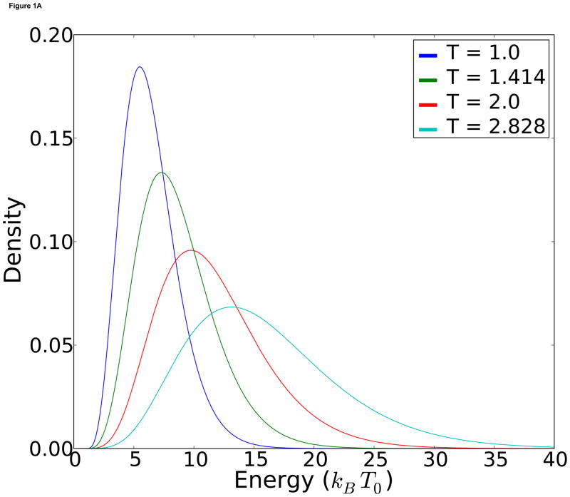
We ran four replicas with temperatures at k_BT =1, 1.414, 2 and 2.828, respectively. Those temperatures follow the geometric recommendation in [28]. In order to get exchanges at a reasonable frequency, we set m = 10, all of the energy functions V_i equal. The probability density functions are shown in Figure 1-A.

Figure 1.

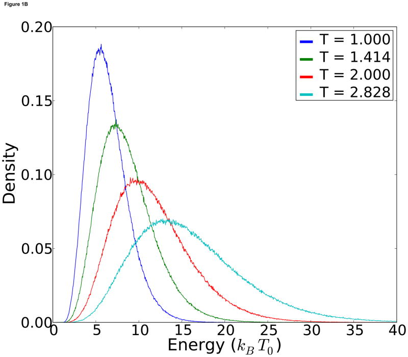
A) Theoretical energy distributions at each temperature. B) Observed temperature distributions for each replica.

Another advantage of MDMS is that energy density graphs such as Figure 1-A can be easily made analytically, and the exchange frequency at equilibrium can be explicitly calculated. When we ran the corresponding RE simulations, we obtain virtually identical energy distributions at each temperature (Figure 1-B).

4. Results and Discussion

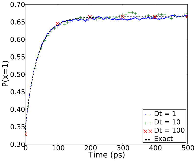
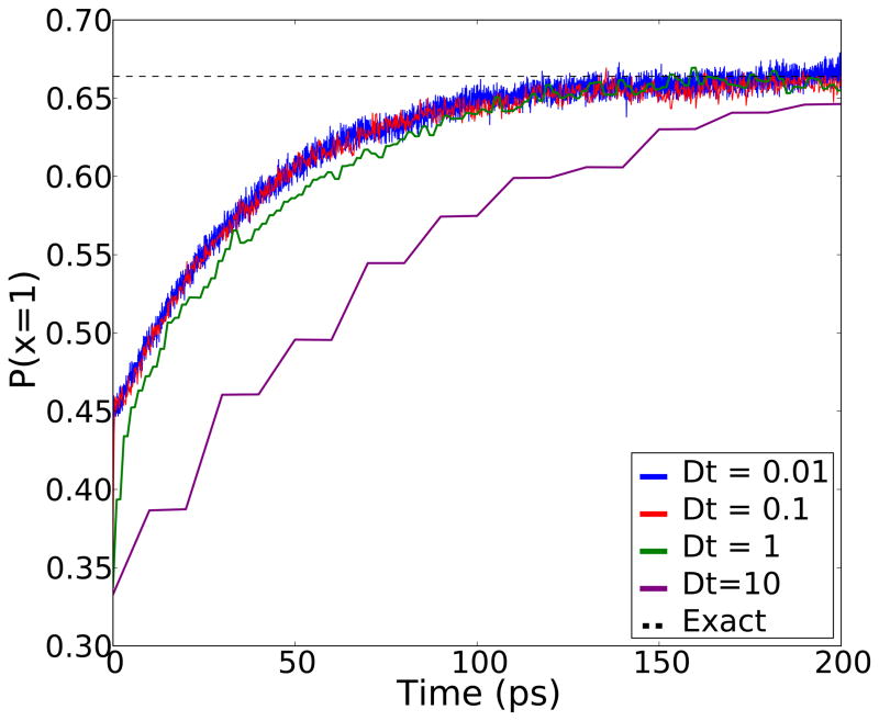
The first test we performed was to see if MDMS can simulate the transitions between local minima effectively. We ran 10,000 independent “MD” simulations, which represent molecular dynamics simulations with no exchanges, for 2000 ps starting from random initial states at a temperature of k_BT = 1. To ensure rapid convergence, we used energy barriers smaller than those listed in Table 1. The reduced barrier heights are listed in the figure legend for Figure 2. We then compared the average population of the lowest energy state (with energy 1 k_BT₀) to the correct equilibrium distribution. Three sets of calculations were performed varying the sampling window δt, and no dependence on δt was observed. This can allow for more challenging systems with even higher barriers between states requiring longer simulation time.

Figure 2.

This figure shows that the standard MD model converges to the correct equilibrium and that the behavior of the system is independent of the sampling window δt. The y-axis is the proportion of simulations where the lowest temperature replica is in the 1st state at time t. The dashed line is the exact solution for uniform initial conditions. For the sake of fast convergence, the energy barriers used were E₁₂ = 6, E₁₃ = 5 and E₂₃ = 2.

To generate representative energies for each replica, we chose the harmonic dimension parameter m = 10 because it gave a reasonable spread without overwhelming the energy gaps. Larger m would simply require smaller gaps between the temperatures of successive replicas, as is seen in practice.

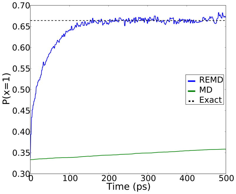
Next we ran RE simulations using four replicas with temperatures k_BT =1, 1.414, 2 and 2.828 respectively. As with the straight MD runs, we averaged 10,000 parallel RE simulations. Independent simulations started with random initial conditions so that each state was uniformly populated. The population of the lowest energy state was compared to the correct equilibrium populations (Figure 3). Figure 3 shows the convergence of the population of the lowest energy state to the analytical result. The simulation energies are shown in Table 1. The standard MD simulations would converge to equilibrium after about 30 ns, while the RE simulations reach their equilibrium values much faster (within 150 exchange attempts) and maintain that population throughout the simulation.

Figure 3.

This figure shows that a simple RE simulation converges significantly faster than an MD simulation with the parameters listed in the table.

To investigate the benefits of frequent exchange attempts, we ran four simulations where we varied the interval between exchange attempts δt. As seen in Figure 4, going from δt = 10 ps to δt = 1 ps shows a pronounced increase in the rate of convergence, in agreement with previous studies [29,30]. However, smaller δt show little additional benefit. There are obvious constraints to the sampling rate, not least of which being the rate of sampling by the highest temperature replica. MDMS is currently limited by the lack of an equilibration time within each well, but this result provides evidence for using frequent exchanges to increase the rate of sampling.

Figure 4.

RE simulations were run with varying exchange frequencies. Convergence rates are increased with faster exchanges, but there is a limit to the rate of convergence leading to diminishing returns.

The last test we ran was to test the recommended temperature intervals from [26]. We assumed that the entropy contribution of the harmonic oscillators was small and only used the entropy from the discrete states for our calculation. As the total entropy is bounded, we were only able to select three temperatures with a constant entropy increase: k_BT =1, 1.414, and 3.4. For comparison, the simulations with geometric temperature differences were run with k_BT =1, 1.414 and 2. Figure 5 shows significantly faster convergence using the constant entropy increase temperature selection. These calculations further show the power of our model in that the total time spent calculating entropies and running simulations was less than three hours.

Figure 5.

RE simulations were run with two different sets of temperature intervals. The first set of simulations were run according to the geometric progression of k_BT =1, 1.414 and 2. The second set were run with a temperature distribution based on [26] with k_BT =1, 1.414 and 3.4.

The simulation results we have presented here are very simple and do not break new ground, but MDMS is very general and can be used to investigate a number of exchange based methods and potentially even more general sampling methods. The model zoo in the supplement gives a small selection of ideas that could be used in developing a systematic test set for new methods. MDMS may become a test-bed for future exchange based sampling methods where many parameters can be tested and evaluated simultaneously.

As one example of a more general exchange method, Hamiltonian RE methods could be implemented by simply modifying the barriers in the rate matrix and using that to define the kinetics of each replica. The reduction in energy barriers could be estimated directly from the particular changes to the energy function or empirically with short simulations. For some types of Hamiltonians, such as changing the dihedral potentials such as in [31], the change in barrier height is easy to calculate. However, even in a less straightforward case, such as changing Lennard-Jones potentials like in [32], potential of mean force calculations could give an estimate for the change in barrier height.

In conclusion, we have presented a new type of model that allows for rapid testing of RE methods. MDMS is a tool that can quickly generate many RE simulations on a pre-defined system with exactly known statistical properties. Results calculated with new methods can be compared to known quantities and guide method development. We intend to use this model to test the applicability of reservoir RE methods [14, 17] and investigate their strengths and weaknesses in a systematic manner.

Highlights.

• We develop a model for testing exchange-based/replica-exchange sampling methods.

• The model can replicate many important features of biologically-relevant proteins.

• The model will greatly increase the speed of development for new replica-exchange-type methods.

References

- 1.Geyer CJ. Computing Science and Statistics. Proc. 23rd Symp. Interface; pp. 156–163. [Google Scholar]
- 2.Hansmann UHE. Chem Phys Lett. 1997;281:140–150. [Google Scholar]
- 3.Sugita Y, Okamoto Y. Chem Phys Lett. 1999;314:141–151. [Google Scholar]
- 4.Zhou R, Berne BJ, Germain R. Proc Natl Acad Sci U S A. 2001;98:14931–14936. doi: 10.1073/pnas.201543998. [DOI] [PMC free article] [PubMed] [Google Scholar]
- 5.Garcia AE, Sanbonmatsu KY. Proteins: Struct, Funct, Bioinf. 2001;42:345–354. doi: 10.1002/1097-0134(20010215)42:3<345::aid-prot50>3.0.co;2-h. [DOI] [PubMed] [Google Scholar]
- 6.Paschek D, Garcia AE. Phys Rev Lett. 2004;93:238105. doi: 10.1103/PhysRevLett.93.238105. [DOI] [PubMed] [Google Scholar]
- 7.Pitera JW, Swope W. Proc Natl Acad Sci U S A. 2003;100:7587–7592. doi: 10.1073/pnas.1330954100. [DOI] [PMC free article] [PubMed] [Google Scholar]
- 8.Sanbonmatsu K, Garca A. Proteins: Struct, Funct, Bioinf. 2002;46:225–234. doi: 10.1002/prot.1167. [DOI] [PubMed] [Google Scholar]
- 9.Fukunishi H, Watanabe O, Takada S. J Chem Phys. 2002;116:9058–9067. [Google Scholar]
- 10.Li H, Li G, Berg BA, Yang W. J Chem Phys. 2006;125:144902. doi: 10.1063/1.2354157. [DOI] [PubMed] [Google Scholar]
- 11.Liu P, Kim B, Friesner RA, Berne BJ. Proc Natl Acad Sci U S A. 2005;102:13749–13754. doi: 10.1073/pnas.0506346102. [DOI] [PMC free article] [PubMed] [Google Scholar]
- 12.Lyman E, Zuckerman DM. J Chem Theory Comput. 2006;2:656–666. doi: 10.1021/ct0600464. [DOI] [PMC free article] [PubMed] [Google Scholar]
- 13.Lyman E, Zuckerman DM. Biophys J. 2006;91:164–172. doi: 10.1529/biophysj.106.082941. [DOI] [PMC free article] [PubMed] [Google Scholar]
- 14.Okur A, Roe D, Cui G, Hornak V, Simmerling C. J Chem Theory Comput. 2007;3:557–568. doi: 10.1021/ct600263e. [DOI] [PubMed] [Google Scholar]
- 15.Okur A, Wickstrom L, Layten M, Geney R, Song K, Hornak V, Simmerling C. J Chem Theory Comput. 2006;2:420–433. doi: 10.1021/ct050196z. [DOI] [PubMed] [Google Scholar]
- 16.Rick SW. J Chem Phys. 2007;126:054102. doi: 10.1063/1.2431807. [DOI] [PubMed] [Google Scholar]
- 17.Roitberg A, Okur A, Simmerling C. J Phys Chem B. 2007;111:2415–2418. doi: 10.1021/jp068335b. [DOI] [PMC free article] [PubMed] [Google Scholar]
- 18.Sugita Y, Kitao A, Okamoto Y. J Chem Phys. 2000;113:6042–6051. [Google Scholar]
- 19.Sugita Y, Okamoto Y. Chem Phys Lett. 2000;329:261–270. [Google Scholar]
- 20.Zuckerman DM. Annual Review of Biophysics. 2011;40:41–62. doi: 10.1146/annurev-biophys-042910-155255. [DOI] [PMC free article] [PubMed] [Google Scholar]
- 21.Brooks BR, Brooks CL, Mackerell AD, Nilsson L, Petrella RJ, Roux B, Won Y, Archontis G, Bartels C, Boresch S, Caflisch A, Caves L, Cui Q, Dinner AR, Feig M, Fischer S, Gao J, Hodoscek M, Im W, Kuczera K, Lazaridis T, Ma J, Ovchinnikov V, Paci E, Pastor RW, Post CB, Pu JZ, Schaefer M, Tidor B, Venable RM, Woodcock HL, Wu X, Yang W, York DM, Karplus M. J Comput Chem. 2009;30:1545–1614. doi: 10.1002/jcc.21287. [DOI] [PMC free article] [PubMed] [Google Scholar]
- 22.Case DA, Cheatham TE, Darden T, Gohlke H, Luo R, Merz KM, Onufriev A, Simmerling C, Wang B, Woods RJ. J Comput Chem. 2005;26:1668–1688. doi: 10.1002/jcc.20290. [DOI] [PMC free article] [PubMed] [Google Scholar]
- 23.Zheng W, Andrec M, Gallicchio E, Levy RM. Proc Natl Acad Sci U S A. 2007;104:15340–15345. doi: 10.1073/pnas.0704418104. [DOI] [PMC free article] [PubMed] [Google Scholar]
- 24.Zheng W, Andrec M, Gallicchio E, Levy RM. J Phys Chem B. 2008;112:6083–6093. doi: 10.1021/jp076377+. [DOI] [PMC free article] [PubMed] [Google Scholar]
- 25.Vanden-Eijnden E, Tal FA. J Chem Phys. 2005;123:184103. doi: 10.1063/1.2102898. [DOI] [PubMed] [Google Scholar]
- 26.Sabo D, Meuwly M, Freeman DL, Doll JD. J Chem Phys. 2008;128:174109. doi: 10.1063/1.2907846. [DOI] [PubMed] [Google Scholar]
- 27.Kone A, Kofke DA. J Chem Phys. 2005;122:206101. doi: 10.1063/1.1917749. [DOI] [PubMed] [Google Scholar]
- 28.Okamoto Y, Fukugita M, Nakazawa T, Kawai H. Protein Eng. 1991;4:639–647. doi: 10.1093/protein/4.6.639. [DOI] [PubMed] [Google Scholar]
- 29.Sindhikara D, Meng Y, Roitberg AE. J Chem Phys. 2008;128:024103. doi: 10.1063/1.2816560. [DOI] [PubMed] [Google Scholar]
- 30.Sindhikara DJ, Emerson DJ, Roitberg AE. J Chem Theory Comput. 2010;6:2804–2808. doi: 10.1021/ct100281c. [DOI] [PubMed] [Google Scholar]
- 31.König G, Boresch S. J Comput Chem. 2011;32:1082–1090. doi: 10.1002/jcc.21687. [DOI] [PubMed] [Google Scholar]
- 32.Hritz J, Oostenbrink C. J Chem Phys. 2008;128:144121. doi: 10.1063/1.2888998. [DOI] [PubMed] [Google Scholar]
Associated Data
This section collects any data citations, data availability statements, or supplementary materials included in this article.