

Abstract
The aim of this study was to display malignant induction probability (MIP) maps alongside dose distribution maps for radiotherapy using X-ray and charged particles such as protons. Dose distributions for X-rays and protons are used in an interactive MATLAB® program (MathWorks, Natick, MA). The MIP is calculated using a published linear quadratic model, which incorporates fractionation effects, cell killing and cancer induction as a function of dose, as well as relative biological effect. Two virtual situations are modelled: (a) a tumour placed centrally in a cubic volume of normal tissue and (b) the same tumour placed closer to the skin surface. The MIP is calculated for a variety of treatment field options. The results show that, for protons, the MIP increases with field numbers. In such cases, proton MIP can be higher than that for X-rays. Protons produce the lowest MIPs for superficial targets because of the lack of exit dose. The addition of a dose bath to all normal tissues increases the MIP by up to an order of magnitude. This exploratory study shows that it is possible to achieve three-dimensional displays of carcinogenesis risk. The importance of treatment geometry, including the length and volume of tissue traversed by each beam, can all influence MIP. Reducing the volume of tissue irradiated is advantageous, as reducing the number of cells at risk reduces the total MIP. This finding lends further support to the use of treatment gantries as well as the use of simpler field arrangements for particle therapy provided normal tissue tolerances are respected.
Improvements in cancer treatments have led to an increase in long-term survival, making it necessary to consider late side effects that may occur many years after treatment, especially in younger patients with curable tumours and who can live for 30–50 years after treatment. Advanced forms of radiotherapy, such as intensity-modulated radiotherapy (IMRT) and charged particle therapy, have entered clinical practice over the last two decades, resulting in more treatment options. To select the best option, the radiation oncologist and physicist should consider not only short-term outcomes but also the longer term effects, such as the probability of inducing secondary malignancies.
The principal aim of this analysis is to calculate and display malignant induction probability (MIP) maps alongside dose maps as a tool to study the potential consequences of different field arrangements and their interactions with radiobiological factors such as fractionation and cellular radiosensitivities. There are reasons to believe that MIP varies non-linearly with dose and that, at higher doses, a reduction in MIP can occur, as originally suggested by the Gray model [1]. Therefore, MIP maps may differ markedly from the corresponding dose maps, making the development of a visualisation tool pertinent. A further aim is to compare the relative risk of malignant induction for two forms of radiation treatment over a three-dimensional (3D) treatment volume, expressed as a ratio of probabilities or as comparative absolute estimates. This work does not presume to predict actual MIP values in humans following radiotherapy, but is intended as a tentative study of the various physical, clinical and biological interactions.
Methods and materials
Description of model
Many mathematical models have been proposed to describe the dose-response relationship for radiation-induced cancer [2-4]. Some models are applicable in low-dose regions and have to be extrapolated to higher doses relevant for radiotherapy [5]. In this study, we have not used a simple linear model, although we intend to incorporate several competing models of malignant induction in a future version of this program. A widely accepted generalised linear quadratic model is detailed in the United Nations Scientific Committee on the Effects of Atomic Radiation [1] and is formulated by combining the probability that a potentially malignant transformation is induced with that of the cell surviving:
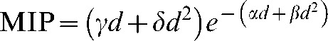 |
(1) |
where α and β are the cell kill parameters, γ and δ are the mutation parameters and d is the dose per fraction.
The model implemented in the present study [6] uses the generalised linear quadratic model with the extra constraints that the mutation and cell kill parameters are linearly correlated with the constant of proportionality x, where x is very small:
| (2) |
| (3) |
This assumption reduces the number of parameters required and has been implicitly incorporated into many models by assuming the same ratio for the mutation and killing parameters [3]. The model considered in the present analysis also incorporates fractionation. This study has not considered the effect of cell repopulation during treatment as, in most instances, the radiation cancer and sarcoma induction will occur in very slowly dividing cell systems such as basal cells of skin, connective tissues, meninges, glial tissues, thyroid and prostate, which emerge from very stable tissues and are associated with low repopulation rates. For tissues that repopulate during radiotherapy, such as bronchial and buccal mucosa and even breast epithelium, an additional time factor may be required [4].
The details of the model are summarised in Appendix A, which leads to the following relationship for mega-voltage X-rays:
 |
(4) |
where Ctr is the mean number of potentially malignant transformed cell, Ptr is the probability of malignant induction per cell, C is the total number of cells at risk and n is the number of fractions.
The inclusion of relative biological effectiveness (RBE) for charged particles is summarised in Appendix B, which leads to the following relationship for charged particles:
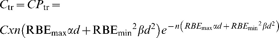 |
(5) |
where RBEmax is the value of RBE in the low-dose limit and RBEmin is the value of RBE in the high-dose limit.
The overall risk of inducing one or more secondary malignancies is given by:
| (6) |
where R0 is the probability of no initiated cells and η is defined as the efficiency for conversion of the transformed cells to become an overt malignancy. The exact value of η is not known but it is expected to be as small as 10−6 [7], so that Equation 6 can then be approximated as:
| (7) |
Therefore, when comparing two different treatment plans for the same patient, the efficiency cancels out and the relative risk becomes simply:
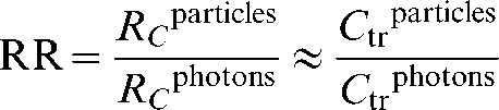 |
(8) |
Note that both x and η cancel out in the equation for relative risk, making the ratio a reliable metric even if there are large uncertainties on these eliminated parameters. Although n also cancels in part of the equation, the fraction number is retained in the exponential portions of the ratio.
Features of the model
The functional form of the MIP dose-response curve is shown in Figure 1a–c for different cell types (i.e. with different α radiosensitivity values) and two different fractionation schemes. The peak MIP will be displaced to higher doses if radiosensitivity is reduced. This is consistent with typical clinical findings of radiosensitive leukaemias occurring at low doses, but more radioresistant sarcomas arising within a high-dose treatment volume. Even in these cases, there is a possibility that such “in-field” cancers arise from fibrous tissues that have replaced a tumour and were themselves not exposed to the full dose since the fibrocytes were originally extratumoural. The MIP curve broadens and shifts to the right when fractionation is increased and, as a result, the maximum MIP occurs at a much higher total dose. For lower penumbral or exit beam doses, the curves shift further to the right, which emphasises the high risk for multiple low-dose exposures within the present model. A quantitative description of the factors that control the position of the turnover point is given elsewhere [6].
Figure 1.

Plots of malignant induction probabilities (MIPs) per cell to show features of the model for X-rays, using Equation A4, for (a) the dose given in a single fraction, (b) an increasing number of 2 Gy fractions and (c) the number of fractions receiving a penumbral dose of 0.2 Gy per fraction. In all cases β=0.03 Gy−2 for all values of α given in the legend and x=1.3×10⁻⁷.
Implementing the model
The malignant induction model is implemented in MATLAB® (MathWorks, Natick, MA) to compare dose and MIP profiles for X-rays and charged particles. The probability of initiating a malignant transformation per cell is calculated on a voxel (volume element)-by-voxel basis, thus taking into account the effects of dose heterogeneity over the entire volume under consideration (detailed in the following sections). The user can enter values for the following parameters: modality (X-rays or charged particles), number of beams (one to four), beam orientation (orthogonal or opposed with appropriate wedge filters), dose per fraction, number of fractions, radiosensitivity parameters and relative biological effectiveness. There is an additional option for a non-specific dose bath specified as a percentage of the prescribed dose given to the entire tissue volume, as described below.
The program work flow is as follows:
Gather user input and pass as arguments to malignant induction function.
Build spatial system matrix representing tumour and normal tissue regions and construct dose map.
Calculate MIP on a voxel-by-voxel basis.
Output the surface plot of the dose over the system, surface of the Ptr over the system and a single value for the total MIP integrated over the entire volume at risk.
System geometry
Two 3D geometrical cases were considered for this analysis and are described in the following sections. For the purposes of this initial study, the normal tissue is assumed to have a homogeneous cell density and type.
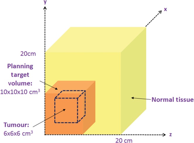
A system geometry was constructed within MATLAB, consisting of a 20×20×20 cm3 cube of normal tissue which houses a 6×6×6 cm3 tumour at its centre (Figure 2). The planning target volume (PTV) includes a 2 cm margin around the tumour to form a PTV of 10×10×10 cm3. For the purposes of this analysis, the region was segmented into voxels; the size of each voxel is 0.5×0.5×0.5 cm3.
Figure 2.
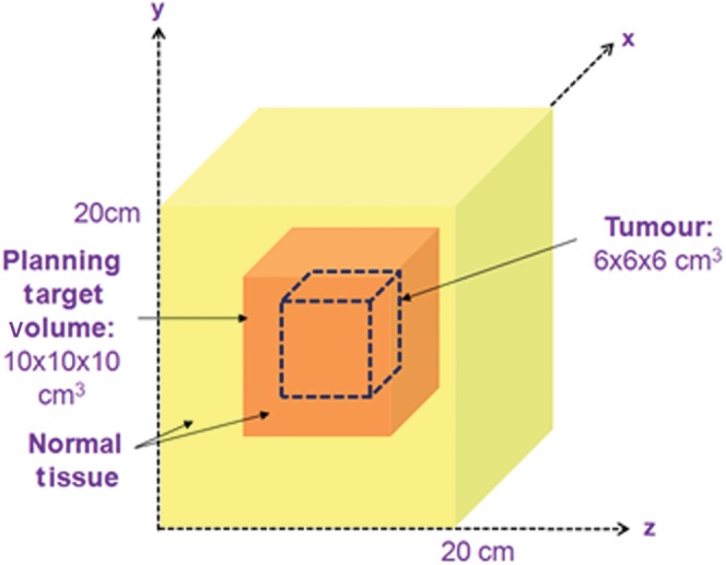
A schematic diagram showing the geometry of the tumour region, planning target volume (PTV) and surrounding normal tissue for a centrally situated tumour and PTV within a 20×20×20 cm3 structure representing normal tissue.
An alternative geometry was also considered in which the PTV was moved towards the corner of the cube of normal tissue, as shown in Figure 3.
Figure 3.
A schematic diagram showing the geometry of the tumour region, planning target volume (PTV) and surrounding normal tissue for a more superficially situated PTV in the corner of the overall normal tissue volume.
Depth dose curves and penumbra
Typical depth-dose curves for megavoltage X-rays and proton-charged particles, shown in Figure 4, have been modelled within MATLAB. Beam widths of 10 cm are applied over the volume to cover the PTV, and a 1 cm penumbra has been added to the left, right, top and bottom of the beam. The voxelised dose distribution is calculated by summing the dose contribution from each beam and normalising to ensure that the prescribed dose is at the centre of the target volume.
Figure 4.
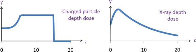
Proton and X-ray beam depth doses, where y is dose and z is depth, used to calculate dose over the volume for the case when the planning target volume is centrally situated.
The MIP per cell (Ptr) for each voxel is calculated from the dose in that voxel and other user-defined input parameters such as the radiosensitivity parameters α and β. These are then combined by integrating over all voxels to give an overall risk of induced secondary malignancy. The number of cells at risk per unit volume of normal tissue has been adjusted so as to provide a reasonable absolute estimate of MIP such as 15–30%, as described elsewhere [6].
Results
The graphical user interface (GUI) of the MIP code is pictured for a three-field proton (Figure 5) and X-ray (Figure 6) anterior and two wedged lateral field plans for a centrally situated PTV. Dose and MIP maps for a horizontal plane through the centre of the target region are displayed along with overall risk and average dose inside and outside the PTV. The user-defined input parameters employed to obtain these results are shown on the GUI and are also detailed in Table 1. It should be noted that the dose within the PTV is more uniform in the proton case, as would be expected, because of the flat, spread out Bragg peaks compared with the dose gradients expected with X-rays, although this range of dose will have little influence on MIP.
Figure 5.

Input parameters, dose and malignant induction maps (colour scale refers to probability in units multiplied by 10−17) and integrated three-dimensional risk values for three beams of protons (two opposed and one orthogonal) targeted at a centrally situated planning target volume (PTV). MIP, malignant induction probability.
Figure 6.

Input parameters, dose and malignant induction maps and integrated three-dimensional risk values (colour scale refers to probability in units multiplied by 10−17) for three beams of X-rays (two wedged lateral fields and an unwedged orthogonal field) for a centrally situated planning target volume (PTV). MIP, malignant induction probability.
Table 1. Input parameters used to calculate results in Table 2 and Figure 7.
| X-rays | Protons | Units | |
| Dose per fraction | 2 | 1.8 | Gy |
| Number of fractions | 20 | 20 | |
| A | 0.15 | 0.15 | Gy−1 |
| B | 0.05 | 0.05 | Gy−2 |
| RBEmin | 1 | 1.05 | |
| RBEmax | 1 | 1.2 |
RBE, relative biological effectiveness.
Table 2 displays the relative risks for malignant induction calculated for protons vs X-rays. For this analysis, between one and four fields were used, as shown in Table 2. In 80% of the cases considered here, X-rays lead to a lower risk of secondary malignancies than protons. For X-rays, the MIP is highly dependent on whether or not the exit dose, which by itself is associated with high MIP, is boosted by an entrance dose from an opposing field.
Table 2. Relative risks for malignant induction (protons vs X-rays), as defined in Equation 8, for a centrally located planning target volume with 10% beam penumbra treated by one, two opposed (2 op), two orthogonal (2 or), three-field or four-field plans. Values greater than unity mean that protons have higher malignant induction probability than X-rays.
| Protons |
|||||
| X-rays | 1 | 2 op | 2 or | 3 | 4 |
| 1 | 0.69 | 1.92 | 1.77 | 2.85 | 3.54 |
| 2 op | 0.86 | 2.38 | 2.19 | 3.54 | 4.40 |
| 2 or | 0.40 | 1.11 | 1.02 | 1.65 | 2.05 |
| 3 | 0.44 | 1.22 | 1.12 | 1.81 | 2.25 |
| 4 | 0.62 | 1.73 | 1.60 | 2.58 | 3.20 |
Figure 7 shows the absolute risk for X-rays and protons for all field configurations considered. For protons, the MIP increases as the number of fields is increased owing to the lower associated entrance doses, meaning that cell killing no longer dominates mutation in the entrance regions. Again, for X-rays, the MIP is highly dependent on whether or not the exit dose, which is associated with high MIP, is buried by an opposing field. The influence of the penumbral dose is also shown.
Figure 7.

Bar charts displaying the percentage risk of secondary malignancy for X-rays and protons using assumptions in Table 1 for each of the different field numbers and their orientations (as in Table 2) in the case of a centrally located planning target volume and where the penumbral dose is either absent or varies from 10% to 50%. The radiobiological and fractionation parameters are as given in Figures 5 and 6. opp., opposed; orth., orthogonal.
The PTV was moved towards the corner of the volume to investigate the effect of absence of dose distal to the spread out Bragg peak for protons (as well as elimination of the entry dose). For this analysis only one-field and two orthogonal field plans were considered. Figure 8 shows the dose and MIP maps for two orthogonal field X-ray and proton plans, but the beam penumbra is not included for either modality in order to simplify the analysis and therefore illustrate the effect of exit dose only (the effect of the beam penumbra is considered further in Figure 7). With these assumptions the only region receiving dose in the proton case is the PTV. This high dose is in the region where cell kill dominates the induction function and, therefore, the MIP is very low. However, with X-rays the exit doses cannot be avoided and they lead to a high MIP.
Figure 8.

Graphs showing dose and malignant induction probability (MIP) maps for a two-field right-angled wedged pair arrangement for X-rays (a) and two-field protons (b) when the planning target volume is moved towards the corner of the overall volume under consideration. Note the three orders of magnitude difference in the MIP scale which vary from multiplication factors of 10−17 for X-rays and 10−20 for protons. The total MIPs are protons 0.11, X-rays 0.25.
As can be observed from Figure 8, in which the PTV is moved towards the corner, the overall MIP is smaller for protons (0.11) than for X-rays (0.25), in some cases by an order of magnitude in each volume element. This is the result of the absence of an exit dose for protons but cannot be avoided when using X-rays. The addition of a penumbra makes little difference to the reduction in relative risk with protons compared with X-rays (as shown in Figure 9) because the risk is influenced to a far greater extent by the high MIP in the exit dose regions.
Figure 9.
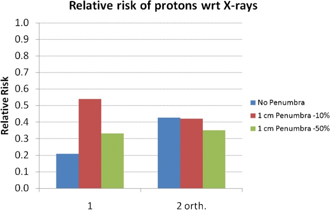
The relative risk of secondary malignancy when using protons instead of X-rays for either single (1) fields or the two-field (2 orth.) plans in the case of a planning target volume situated towards the corner of the overall volume and for different assumptions as to penumbral dose. wrt, with respect to.
Sensitivity of MIP to changes in cell radiosensitivity
The effect of changing cell radiosensitivity on MIP was assessed for the three-field case in which the PTV is in the centre of the overall volume, for both protons and X-rays. In reality, the protons may fare better if only two fields can be used, so that these calculations represent a poor case scenario for protons. For this analysis, no penumbra was applied to the beams. Figure 10 shows the total MIP, integrated over the whole region at risk, for four different values of the normal tissue radiosensitivity parameter α (0.15, 0.1, 0.05, 0.01), where the α/β ratio is 3 for all values of α. For X-rays, as the radiosensitivity increases MIP decreases as the dose is high enough to be over the peak in MIP. For protons, the dose deposited in normal tissues is lower, and, therefore, increasing the normal tissue radiosensitivity increases MIP to a maximum followed by a subsequent decrease. Owing to the presence of an exit dose for X-rays, a larger volume of normal tissue is unavoidably irradiated and, consequently, the maximum MIP value is higher for X-rays than for protons, but it falls sharply with increasing radiosensitivity.
Figure 10.
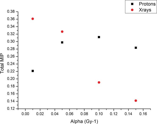
Plot of total malignant induction probability (MIP) for the three-field plans for X-rays and protons (as in the treatment geometry of Figures 5 and 6 and for the same dose parameters) for different values of the radiosensitivity parameter α. The α/β ratio is 3 for all values of α.
Adding a dose bath
In order to model the effect of a non-targeted dose “bath” of radiation over the whole region, separate studies were performed in which a user-defined percentage of the target dose could be applied uniformly over the whole normal tissue 20×20×20 cm3 region, typically to 5–10% of the PTV dose. In all cases tested for each of the beam arrangements used in the above examples, it was found that this had the effect of increasing the MIP by as much as an order of magnitude. Only detrimental effects were found. This finding could have serious implications for IMRT and tomotherapy, in which large volumes of tissue are irradiated to a low to moderate dose [8].
Discussion
The results presented are dependent on the validity of the linear quadratic model and the additional assumptions made. Different predictive models of carcinogenesis will inevitably give different results, and we have selected a model that may have advantages for the study of radiotherapy compared with the standard radiation protection models. Another potential issue is age dependency, but the yield of cancers can be varied by changing the radiosensitivity parameters, which could in principle be linked to age.
The model used produces increasing MIP where the dose increases enough to cause significant transformation but is not high enough to nearly always cause death of the transformed cell. The physical doses that correspond to high MIP will vary depending on the radiosensitivity of the cells under irradiation. It should be noted that, although high doses seem advantageous in terms of MIP, they are not advantageous in terms of normal tissue complication probability. Treatment geometry, including the length and volume of tissue traversed by each beam, can have a large effect on MIP, and it is clear that reducing the volume of tissue irradiated is advantageous, as reducing the number of cells at risk reduces the total MIP. For X-rays the MIP is highly dependent on whether or not the exit dose, which is associated with a high MIP, is contained within another opposed field. This could have repercussions for IMRT [9], in which there are large volumes of exit beams that do not overlap with other beams. In the case of tomotherapy, there will also be a large volume of tissue irradiated at low to moderate dose. This has been studied using the standard radiation protection model [9], which assumes a linear dose-response relationship that is valid only to 4 Gy and is perhaps unsuited to access MIP following radiotherapy.
Validation of the functional form of the dose-response relationship is necessary to have confidence in the relative risks of secondary malignancy produced in this analysis, as with all other proposed models of carcinogenesis. Evidence for maxima in the dose-response curves followed by a subsequent decrease with dose has been documented in certain cell lines [10,11] and also in some rodent studies in vitro [12]. Whether or not this can be extended to human tissues and organs at risk remains to be validated. Attempts were made by the authors to locate relevant data and produce fits using the model, but large uncertainties on the data points made it difficult to draw firm conclusions. It was also difficult to test the dose-response curve clinically because of the lack of available treatment plans for the primary treatment that were then linked to the secondary cancer occurrence. It is hoped that the obvious need to understand radiation-induced malignancy will encourage the storage of the appropriate prospective clinical data in 3D format.
This analysis has provided an open source visualisation tool for MIP and dose and it is considered important that future treatment planning software be capable of displaying graphs of biological end points such as surviving fraction and MIP as well as physical dose. Work is currently under way to apply this and alternative MIP models to clinical treatment plans and produce dose, MIP and surviving fraction maps alongside each other with a view to later publications.
The model presented in this paper can potentially be extended to heavier charged particles such as alpha particles and carbon ions by modifying the RBEmin and RBEmax within the radiobiological models as well as the physical dose distributions.
Conclusions
It cannot be assumed that using charged particles rather than X-rays always lead to a reduction in the risk of secondary malignancies. Charged particle therapy should use as few beams as possible to reduce the volume of cells irradiated, with minimal normal tissue traversal (the use of rotating gantries would help in this respect). More work is necessary to fully validate and develop the model and to apply it to clinical treatment plans. Predictions of the model should be subjected to confirmation by modern cellular and tissue experiments along with clinical outcomes.
In the future it is hoped that fully validated MIP calculations can be incorporated into treatment planning software and a multiparameter optimisation performed including tumour cure probability, normal tissue complication probability and MIP with weighting factors dependent on the latency of the effects. Although an accurate calculation of absolute malignant risk is possibly unattainable because of the large number of factors involved, the relative risk between two treatment plans for the same patient will hopefully be a useful and reliable comparative metric in the not too distant future.
Acknowledgments
The authors wish to thank the Martin Oxford School for funding the Particle Therapy Cancer Research Institute (PTCRi); Anne Trefethen, the director of the Oxford e-Research Centre, who co-supervised Mark Houtston on this project; and Ken Peach, who is co-director of the PTCRi.
Appendix A
Malignant induction probability model
Using the linear quadratic model [13], the number of lethal chromosome breaks per cell (A) can be represented by:
| (A1) |
where n is the number of fractions, d is the dose per fraction and α and β are radiosensitivity parameters for cell killing.
The probability of inducing a potentially malignant transformation (Ptr) can be represented by the product of the probabilities of induction (PI) and survival (PS). Assuming that lethal and non-lethal chromosome aberrations are Poisson distributed, these probabilities can be expressed as:
| (A2) |
where A is the mean expected number of lethal chromosome aberrations per cell.
Because malignant induction is a rare event, the assumption is made that xA is <<1 and therefore the induction probability can be approximated as follows:
| (A3) |
Thus the probability of at least one malignant transformation in a surviving cell can be expressed as:
 |
(A4) |
The mean number of potentially malignant transformed cells (Ctr) can be calculated from the probability per cell (Ptr) and the total number of cells at risk (C):
 |
(A5) |
Appendix B
Inclusion of relative biological effectiveness
For the special case of radiations which contain, at least partly, high linear energy transfer (LET) radiation, such as protons and ions, the RBE must be taken into account [14]:
 |
(A6) |
where RBEmax is the value of RBE in the low-dose limit:
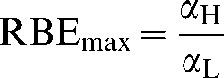 |
(A7) |
and RBEmin is the value of RBE in the high-dose limit:
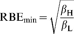 |
(A8) |
The subscripts L and H refer to low and high LET.
References
- 1.United Nations Scientific Committee on the Effects of Atomic Radiation Genetic and somatic effects of ionizing radiation. Annex B. Dose-response relationships for radiation-induced cancer. Vienna, Austria: UNSCEAR; 1986 [Google Scholar]
- 2.Lindsay KA, Wheldon EG, Deehan C, Wheldon TE. Radiation carcinogenesis modelling for risk of treatment-related second tumours following radiotherapy. Br J Radiol 2001;74:529–36 [DOI] [PubMed] [Google Scholar]
- 3.Dasu A, Toma-Dasu I, Olofsson J, Karlsson M. The use of risk estimation models for the induction of secondary cancers following radiotherapy. Acta Oncol 2005;44:339–47 [DOI] [PubMed] [Google Scholar]
- 4.Sachs RK, Shuryak I, Brenner D, Fakir H, Hlatky L, Hahnfeldt P. Second cancers after fractionated radiotherapy: Stochastic population dynamics effects. J Theor Biol 2007;249:518–31 [DOI] [PMC free article] [PubMed] [Google Scholar]
- 5.Schneider U, Lomax A, Lombriser N. Comparative treatment planning using secondary cancer mortality calculations. Phys Med 2001;17 Suppl 1:97–9 [PubMed] [Google Scholar]
- 6.Jones B. Modelling carcinogenesis after radiotherapy using Poisson statistics: implications for IMRT, protons and ions. J Radiol Prot 2009;29:1–15 [DOI] [PubMed] [Google Scholar]
- 7.United Nations Scientific Committee on the Effects of Atomic Radiation Sources and effects of ionising radiation. Annex E. Mechanisms of radiation oncogenesis. Report to the General Assembly. New York, NY: UNSCEAR; 1993 [Google Scholar]
- 8.Hall EJ. Intensity-modulated radiation therapy, protons, and the risk of second cancers. Int J Radiat Oncol Biol Phys 2006;65:1–7 [DOI] [PubMed] [Google Scholar]
- 9.Davis S, Evans C, Jones P, Gagliardi F, Haynes M, Hunter A, et al. The effect of intensity-modulated radiotherapy on radiation-induced second malignancies. Int J Radiat Oncol Biol Phys 2008;70:1530–6 [DOI] [PubMed] [Google Scholar]
- 10.Borek C, Hall EJ. Transformation of mammalian cells in vitro by low doses of X-rays. Nature 1973;243:450–3 [DOI] [PubMed] [Google Scholar]
- 11.Suit H, Goldberg S, Niemierko A, Ancukiewicz M, Hall E, Goitein M, et al. Secondary carcinogenesis in patients treated with radiation: a review of data on radiation-induced cancers in human, non-human primate, canine and rodent subjects. Radiat Res 2007;167:12–42 [DOI] [PubMed] [Google Scholar]
- 12.Sasaki S, Fukuda N. Dose-response relationship for induction of solid tumors in female B6C3F1 mice irradiated neonatally with a single dose of gamma rays. J Radiat Res (Tokyo) 1999;40:229–41 [DOI] [PubMed] [Google Scholar]
- 13.Lea DE. Actions of radiations on living cells. Cambridge, UK: Cambridge University Press; 1946 [Google Scholar]
- 14.Carabe-Fernandez A, Dale R, Jones B. The incorporation of the concept of minimum RBE (RBEmin) into the linear-quadratic model and the potential for improved radiobiological analysis of high-LET treatments. Int J Radiat Biol 2007;83:27–39 [DOI] [PubMed] [Google Scholar]