Sonoanatomy relevant for ultrasound-guided central neuraxial blocks via the paramedian approach in the lumbar region

Abstract

Objectives

The use of ultrasound to guide peripheral nerve blocks is now a well-established technique in regional anaesthesia. However, despite reports of ultrasound guided epidural access via the paramedian approach, there are limited data on the use of ultrasound for central neuraxial blocks, which may be due to a poor understanding of spinal sonoanatomy. The aim of this study was to define the sonoanatomy of the lumbar spine relevant for central neuraxial blocks via the paramedian approach.

Methods

The sonoanatomy of the lumbar spine relevant for central neuraxial blocks via the paramedian approach was defined using a “water-based spine phantom”, young volunteers and anatomical slices rendered from the Visible Human Project data set.

Results

The water-based spine phantom was a simple model to study the sonoanatomy of the osseous elements of the lumbar spine. Each osseous element of the lumbar spine, in the spine phantom, produced a “signature pattern” on the paramedian sagittal scans, which was comparable to its sonographic appearance in vivo. In the volunteers, despite the narrow acoustic window, the ultrasound visibility of the neuraxial structures at the L3/L4 and L4/L5 lumbar intervertebral spaces was good, and we were able to delineate the sonoanatomy relevant for ultrasound-guided central neuraxial blocks via the paramedian approach.

Conclusion

Using a simple water-based spine phantom, volunteer scans and anatomical slices from the Visible Human Project (cadaver) we have described the sonoanatomy relevant for ultrasound-guided central neuraxial blocks via the paramedian approach in the lumbar region.

Ultrasound is frequently used to guide central venous cannulation [1] and peripheral nerve blocks [2,3]. However, published data suggest that it is rarely used for imaging the spine or for central neuraxial blocks (CNBs; epidural and spinal injections) [4], which is surprising considering that there are data suggesting that an ultrasound examination prior to epidural access (pre-puncture scan, preview scan or scout scan) improves technical [5-7] and clinical [7,8] outcomes and also the learning curve of obstetric epidural anaesthesia [9]. Despite these encouraging results, we believe that there are very few anaesthetists who currently perform a preview scan prior to epidural catheterisation [5,7] or real-time ultrasound-guided (USG) CNBs [6,10]. This is quite interesting considering that emergency physicians are able to interpret ultrasound images of the spine [11] and are performing lumbar puncture using ultrasound in the accident and emergency department [11,12]. Reasons for this paucity of data or a lack of interest in USG CNBs in regional anaesthesia are not clear, but the authors believe it may be due to a lack of understanding of spinal sonoanatomy. The aim of this study was to describe the sonoanatomy relevant for USG CNBs via the paramedian approach in the lumbar region.

Methods and materials

This study was conducted in three parts. The first part involved the use of a “water-based spine phantom”, which we have previously described [13], to determine if it was possible to identify the sonographic appearance of the osseous elements of the lumbar spine in the spine phantom during a paramedian sagittal scan. The paramedian axis was chosen for the scan because it is superior to the median transverse and median sagittal axis for visualising the neuraxial anatomy [14]. The second part of the study aimed to compare (visually) the sonographic appearance of the osseous elements from the spine phantom with in vivo images of these structures, and to determine if it was possible to identify the neuraxial structures (ligamentum flavum, posterior dura, epidural space, intrathecal space and the cauda equina) during a paramedian sagittal scan of the lumbar spine in volunteers. The third part of the study involved defining the sonoanatomy of the osseous elements and neuraxial structures of the lumbar spine using anatomical slices that were obtained from the Visible Human Project male data set (cadaver).

Study involving the water-based spine phantom

The water-based spine phantom was prepared by immersing a lumbosacral spine model (Sawbones; Pacific Research Laboratories Inc., Vashon, WA), with the spinous processes directed towards the ceiling, in a water bath (length×width×height: 60×40×25 cm) so that 1–2 cm of water was above the tip of the spinous processes (Figure 1). As the spine model is made of a buoyant material (foam cortical shell), a weight had to be attached to its undersurface to make it sink. The spine model was then scanned, with the transducer in contact with the surface of the water, in the paramedian sagittal axis using a Micromaxx (Sonosite Inc., Bothell, WA) ultrasound system with image-recording capabilities and a curved array transducer (5-2 MHz) with its orientation marker directed cranially. The latter was used for the scan because the spine and neuraxial structures are located at a depth of approximately 5–7 cm in adults, and low-frequency ultrasound that penetrates deeper into body tissues than high-frequency ultrasound is best suited for imaging the spine. Moreover, the divergent ultrasound beam from a curved array transducer also produces a wide field of vision, which is ideal when one performs real-time USG CNBs [10].

Figure 1.

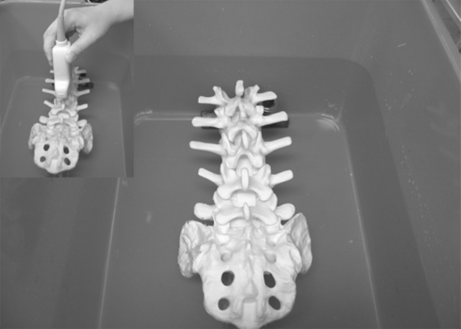
The water-based spine phantom. Note how the lumbosacral spine model was immersed in water. Inset shows how the ultrasound scan was performed through the water.

The L3/L4 and L4/L5 intervertebral spaces were chosen as the targets for the scan in the spine phantom because the majority of central neuraxial blocks in clinical practice are performed at these levels. It was easy to locate the target intervertebral spaces in the spine phantom because one could see them through the water. A paramedian sagittal scan of each of the osseous elements (lamina, articular process and the transverse process) at the target intervertebral spaces was then performed with a marker (22 G spinal needle) in contact with the structure (Figures 2–4). The marker not only ensured that the correct osseous structure was being scanned but also allowed us to validate their sonographic appearance. The same is not possible in vivo, and one has to rely on identifying the sacrum and the L5/S1 gap before counting upwards to locate the desired intervertebral space [10,15]. Therefore, a paramedian sagittal scan of the L5/S1 gap in the spine phantom was also performed to characterise this landmark (Figure 5a).

Figure 2.

Paramedian oblique sagittal sonogram of the lamina (L3, L4, L5) from (a) the water-based spine phantom and (b) volunteers, and a representative anatomical slice from (c) the Visible Human Project (cadaver). In the latter, the lamina has been shaded in green (c). Note the marker (needle) in contact with the lamina in the water-based spine phantom (a). This was done to ensure that the lamina was being scanned and also helped in validating its sonographic appearance. A graphic overlay has been placed over the lamina in (a) to illustrate the “horse head sign”. AC, anterior complex; CE, cauda equina; ES, epidural space; ESM, erector spinae muscle; ILS, interlaminar space; ITS, intrathecal space; IVD, intervertebral disc; LF, ligamentum flavum; PD, posterior dura; SC, spinal canal; VB, vertebral body.

Figure 4.

Paramedian sagittal sonogram of the transverse process from the (a) water-based spine phantom, (b) volunteers and (c) the Visible Human Project (cadaver) In the latter, the transverse processes of L3 and L4 have been shaded in green (c). Note how the acoustic shadow of the TPs produces the “trident sign” [3]. ESM, erector spinae muscle; PM, psoas muscle; TP, transverse process.

Figure 5.

Paramedian sagittal sonogram of the L5/S1 gap from the (a) water-based spine phantom, (b) volunteers and (c) the Visible Human Project (cadaver). In the latter, the lamina of L4 and L5 vertebra and the posterior part of the sacrum have been shaded in green (c). CE, cauda equina; ESM, erector spinae muscle; ITS, intrathecal space; PD, posterior dura; VB, vertebral body.

Volunteer study

After research ethics committee (The Joint Chinese University of Hong Kong — New Territories East Cluster Clinical Research Ethics Committee, Hong Kong) approval, and written informed consent, six healthy young volunteers were recruited for this study. Exclusion criteria included a body mass index (BMI) >35 kg m⁻², clinically obvious or known spinal deformity and previous spine surgery. All the ultrasound scans were performed by a single investigator (MKK), who was experienced in spinal sonography [10], with the volunteer lying comfortably on a bed in the left lateral position. The hips and knees of the volunteer were also flexed to mimic the position normally adapted during CNB. A Micromaxx ultrasound system with a curved array transducer (C60e; 5-2 MHz) was used for the scan. A liberal amount of ultrasound gel was applied to the skin over the lumbar region for acoustic coupling and a paramedian sagittal scan of the non-dependent side of the lumbar spine was performed. The transducer was positioned 1–2 cm lateral to the spinous processes with its orientation marker directed cranially (paramedian sagittal scan). The transducer was also tilted slightly medially during the scan so that the ultrasound beam was insonated in a paramedian oblique sagittal plane. This was done to ensure that the incident ultrasound beam entered the spinal canal through the widest part of the interlaminar space. The scanning depth was set to 9.2 cm and the ultrasound image was optimised by manually adjusting the gain to obtain the best possible image. The sacrum was initially identified as a flat hyperechoic structure with a large acoustic shadow anterior to it (Figure 5b). The transducer was then slowly moved cranially, maintaining the same orientation, until the L5/S1 gap was seen (Figure 5b). Thereafter the L3/L4 and L4/L5 interlaminar spaces were identified by counting upwards (Figure 2b). The ultrasound images during the entire scan in each volunteer were recorded on tape using a digital video camera recorder (DCR-PC9E; Sony Corporation, Tokyo, Japan) via the video output port of the ultrasound machine.

The following parameters were recorded during the volunteer scan. The visibility of the neuraxial structures (lamina, ligamentum flavum, interlaminar space, epidural space, posterior dura, intrathecal space, cauda equina, pulsations of the cauda equina, anterior dura-posterior longitudinal ligament–vertebral body complex) at the L3/L4 or L4/L5 lumbar interspace (whichever had the best visibility) were scored in real time by the same investigator who performed the ultrasound scan (MKK). A four-point numerical scale (0=not visible, 1=hardly visible, 2=well visible, 3=very well visible) [6,10] was used for the assessment and the total ultrasound visibility score (UVS) was calculated for every subject (maximum score possible=27). The scan was considered a success if the lamina and at least one deep soft tissue structure was visualised. The ultrasound visibility of the neuraxial structures was judged to have been good if the mean total UVS was >18, average if the score was 9–18 and poor if the score was <9 [10].

Vertical and oblique distances from the skin to the lamina and the posterior dura, areas of the acoustic shadow (produced by a single lamina; Figure 6) and the acoustic window (between two adjacent acoustic shadows; Figure 7) were also measured using an “off-cart” method. Still images (TIFF; 720×576 pixels and 8-bit grey levels) were captured from the video recordings using Adobe Premier Pro 2.0 (Adobe Systems Inc., San Jose, CA), and Image-Pro Plus 6.2 (Media Cybernetics, Silver Spring, MD) was used for the off-cart measurements. A spatial scale (pixels per centimetre) was calibrated in Image-Pro Plus (IPP) before the distance and area measurements were made. In the spatial calibration dialogue box of IPP the centimetre was selected as the unit for measurement. Thereafter, the number of pixels per centimetre in the horizontal (x) and vertical (y) axes of the ultrasound image (36 pixels cm^–1) were determined by setting the calibration scale to match the depth scale (9.2 cm, object of known size) marked on the ultrasound image. The spatial scale that we calibrated in this study was different from that used in our previous report (Sonosite C60e: 46.3 pixels cm^–1) [10], despite using the same ultrasound system and transducer, because the scanning depths used in the two studies were different (9.2 vs 7.2 cm), and a change in depth is known to affect the lateral resolution of an ultrasound image. To measure distance, the spatial scale was selected and a straight line was connected between two anatomical landmarks. The distance between these two points was expressed in centimetres [10]. For area measurement, a polygonal region of interest (ROI) was selected over the outlines of the acoustic shadow and window in the ultrasound image using the free hand irregular ROI tool in IPP. During this process the lighting in the room was dimmed to reduce glare and improve the delineation of the outlines of the acoustic shadow and window in the ultrasound images. Thereby a coloured area was produced within the ROI and the area of this ROI was measured and expressed in cm².

Figure 6.

Paramedian oblique sagittal sonogram of the lumbar spine at the L3/L4/L5 level. Note the acoustic shadow of the lamina and the acoustic window, which results from reflections of the ultrasound signal from the neuraxial structures within the spinal canal. ILS, interlaminar space.

Figure 7.

Paramedian oblique sagittal sonogram of the lumbar spine at the L3/L4/L5 level. The posterior epidural space is seen as a hypoechoic space (a few millimetres wide) between the hyperechoic ligamentum flavum and the posterior dura. Note that the posterior dura appears brighter and is also better visualised than the ligamentum flavum in this sonogram. ESM, erector spinae muscle; ILS, interlaminar space; LF, ligamentum flavum.

Echo-intensity of the ligamentum flavum (LF) and posterior dura (PD) was then measured using computer-assisted greyscale analysis (Adobe Photoshop CS2; Adobe System Inc.) [16,17] by a computer technician who was otherwise not involved with the study. Still images (TIFF; 720×576 pixels and 8-bit grey levels) that were previously captured from the video recordings were imported into Adobe Photoshop CS2 and were normalised to ensure that the brightness and contrast of the whole image was at the same level before any greyscale median (GSM) measurement. A polygonal ROI box (100×100 pixels) was placed over the LF and a ROI box (25×25 pixels) was placed over the PD. While placing these ROI boxes in the LF or PD, care was taken to ensure that they were placed over an area that appeared brightest to the naked eye. The mean [standard deviation (SD)] and median (range) values of greyscale intensity or echo-intensity of the pixels inside the ROI were determined using the standard histogram function in Adobe Photoshop CS2. An echo-intensity value of 0 represents “pure black” and a value of 255 represents “pure white”.

Study involving the Visible Human Project

Anatomical slices (Figures 2–5) corresponding to the paramedian sagittal and paramedian oblique sagittal scans described above were obtained from the Visible Human Project male data set. The Java applet in the Visible Human Server at EPFL (École Polytechnique Fédérale de Lausanne) was used to navigate through the data set and render the anatomical slices that closely resembled the ultrasound scans described above (Figures 2–5). The sonoanatomy of the osseous elements in the spine phantom and neuraxial structures in the volunteer scans were then defined (visually) in the anatomical slices.

Statistical analysis

The data were analysed using SPSS for Windows (v. 14; SPSS Inc., Chicago, IL). The Kolmogorov–Smirnov test was used to test the normality of the data recorded. The data are presented as the mean (SD) when normally distributed and as median (range) when not normally distributed. For statistical comparison, the paired samples t-test was used to compare the data when they were normally distributed and the Wilcoxon signed-rank test when the data were not normally distributed. A p-value <0.05 was considered statistically significant.

Results

The osseous elements of the lumbar spine, in the water-based spine phantom, produced hyperechoic reflections against the anechoic background of water (Figures 2–5). Individual osseous elements could be clearly visualised, and representative ultrasound images of the L5/S1 gap (Figure 5a), lamina (Figure 2a), articular process (AP; Figure 3a) and the transverse process (Figure 4a), from the spine phantom, are presented in Figures 2–5. The sacrum was identified as a flat hyperechoic structure with a large acoustic shadow anterior to it. A gap was seen between the lamina of L5 and the sacrum, which was the L5/S1 gap (Figure 5a). The lamina produced a pattern that resembled the head and neck of a horse, which we refer to as the “horse head sign” (Figure 2a), and the gap between adjoining lamina was the interlaminar space (Figure 2a). The APs appeared as one continuous hyperechoic wavy line with no intervening gaps (Figure 3a) and the transverse process appeared as a crescent-shaped hyperechoic reflection with its concavity facing anteriorly (Figure 4a).

Figure 3.

Paramedian sagittal sonogram of the articular process from the (a) water-based spine phantom and (b) volunteers, and a representative anatomical slice from (c) the Visible Human Project (cadaver). A graphic overlay has been placed in (b) to illustrate the camel-hump-like appearance of the articular processes (the camel hump sign). AP, articular process; ESM, erector spinae muscle; FJ, facet joint; VB, vertebral body.

A paramedian sagittal scan of the lumbar spine was successfully performed in 3 male and 3 female volunteers with a mean (SD; range) age of 22.7 (1.2; 21–24) years, weight 52.3 (6.2; 46–60) kg, height 167.3 (6.9; 159–175) cm and BMI of 18.5 (1.2; 17–20.3) kg m⁻². The ultrasound visibility of the neuraxial structures at the L3/L4 or L4/L5 intervertebral space was judged as good and the mean (SD) total UVS was 22.5 (2.26). The osseous elements of the lumbar spine that were clearly delineated during the paramedian sagittal scan in the volunteers were the lamina, interlaminar space, AP and the transverse processes, and they were visually comparable in appearance to those visualised in the water-based spine phantom (Figures 2–5). The acoustic shadow of the transverse processes and the psoas muscle in the intervening acoustic window produced the “trident sign” (Figure 4b) that we have previously described [3]. Representative images of these structures from the spine phantom, volunteers and the Visible Human Project (cadaver) are shown in Figures 2–5.

During the paramedian sagittal scan, the lamina was the first osseous structure visualised. Since bone impedes the transmission of ultrasound there was an acoustic shadow anterior to each lamina (Figure 6). In between the dark acoustic shadows of adjacent lamina there was a rectangular area in the sonogram where the neuraxial structures were visualised. This was the acoustic window and resulted from reflections of the ultrasound signal from the neuraxial structures within the spinal canal (Figure 7). The area of the acoustic shadow [mean (SD; 95% confidence interval): 15.1 (1.28; 13.8–16.5) cm²] was significantly greater (p=0.001) than that of the acoustic window [11.0 (0.91; 10.0–12.0) cm²]. In the acoustic window the ligamentum flavum was seen as a hyperechoic band across adjacent lamina (Figure 7). Anterior to the ligamentum flavum, the posterior dura was also seen as a hyperechoic structure and the epidural space was the hypoechoic space (a few millimetres wide) between the ligamentum flavum and the posterior dura (Figure 7). The ligamentum flavum and the posterior dura were both hyperechoic in appearance, but the median (range) ultrasound visibility score of the posterior dura [3 (2-2)] was significantly greater (p=0.04) than that of the ligamentum flavum [2 (2-2)], and the mean (SD) echo-intensity of the posterior dura [129.1 (23.9)] was also significantly greater (p=0.009) than that of the ligamentum flavum [85.9 (16.4)]. The posterior epidural space was also visualised in all our volunteers. The thecal sac with the cerebrospinal fluid was seen as an anechoic space anterior to the posterior dura, and the cauda equina, which was located within the thecal sac, was seen as multiple horizontal hyperechoic shadows within the anechoic thecal sac, with a median (range) visibility score of 1 (1–3). Pulsations of the cauda equina were also identified in 5 out of the 6 (83.3%) volunteers studied. The anterior dura was also hyperechoic, but we were unable to differentiate it from the posterior longitudinal ligament and the posterior surface of the vertebral body as they were of the same echogenicity (isoechoeic) and very closely apposed to each. This produced a single, composite, hyperechoic reflection anteriorly that we refer to as the “anterior complex” (Figure 7). The distances measured from the skin to the lamina and the posterior dura were also significantly greater (p<0.001) in the oblique axis than in the vertical axis (Table 1).

Table 1. Vertical and oblique distances from the skin to the lamina and posterior dura.

Measurements	Vertical	Oblique	p-value
Distance from skin to the lamina (cm)	2.54 (0.31) 2.21–2.87	3.59 (0.47) 3.10–4.08	0.002
Distance from skin to the posterior dura (cm)	3.19 (0.48) 2.69–3.69	4.66 (1.17) 3.44–5.88	0.005

Data are presented as mean (standard deviation) confidence interval.

Discussion

In this study we have described the sonoanatomy relevant for USG CNBs via the paramedian approach in the lumbar region using a water-based spine phantom, volunteers and anatomical slices from the Visible Human Project (cadaver). We found that the water-based spine phantom was a simple model to define the osseous anatomy of the lumbar spine. Each osseous element of the spine produced a “signature pattern” on the ultrasound scan and they were comparable to their sonographic appearance in vivo. In the volunteer scans, despite the narrow acoustic window, the ultrasound visibility of the neuraxial structures was good and we were able to delineate the sonoanatomy relevant for CNBs.

Our results must be interpreted after considering the limitations of this study. The neuraxial structures were identified and scored for their visibility in the volunteers by a single unblinded observer. Moreover, this was not verified against an alternative imaging modality such as MRI, but was based on our experience [10], understanding of spinal sonography from previously published data [6,14,18] and cadaveric anatomy from the Visible Human Project. We also did not perform transverse scans to correlate the sonoanatomy visualised in the paramedian oblique sagittal scans. Currently there are no data validating the ultrasound appearances of neuraxial structures in the lumbar region, and future research in this area is warranted. The system settings in an ultrasound system (e.g. gain, dynamic range, depth of scan, frequency setting etc.) can affect the greyscale intensity of an ultrasound image. However, these parameters were not standardised for the computer-assisted greyscale analysis in this study because we wanted to mimic the clinical situation when a ultrasound image is optimised by making necessary adjustments to the system settings.

The water-based spine phantom was simple to set up and a paramedian sagittal scan through the anechoic water produced high-quality ultrasound images of the osseous elements of the spine. Each osseous element produced a very characteristic appearance or pattern on the sonogram, and all were comparable to those seen in the volunteer scans and were easily defined in the anatomical slices. We are not aware of any published data describing the use of a similar model to study the sonoanatomy of the lumbar spine, although scanning a single lumbar (L3) vertebra through water [19], or a cervical spine model embedded in a jelly preparation [20] to define the relevant spinal sonoanatomy previously been described. Today, there are models to learn musculoskeletal ultrasound imaging techniques (using human volunteers), the sonoanatomy relevant for peripheral nerve blocks (using human volunteers or cadavers) and the required interventional skills (using tissue-mimicking phantoms) to perform ultrasound guided regional anaesthetic techniques. However, there are very few models or tools available to learn spinal sonography or ultrasound-guided central neuraxial blocks. The water-based spine phantom was very useful for this purpose as it allowed us to delineate the sonographic appearance of the osseous elements of the spine. Being able to recognise these sonographic patterns is, in our opinion, the first step in learning how to interpret ultrasound images of the spine. The water-based spine phantom also offered several other advantages. It was relatively cheap, could be quickly set up, could be repeatedly used without worrying about it deteriorating or decomposing as tissue-based phantoms do, and one could also use it to practise needling techniques (in plane or out of plane). These features make the water-based spine phantom a valuable tool for teaching and learning spinal sonography. Future research should evaluate its effect on the learning curve of spinal sonography and ultrasound-guided central neuraxial interventions.

The area of the acoustic shadow was significantly greater than the area of the acoustic window in our volunteer scans. This was an expected finding because the spine is mostly made up of bone, and bone impedes the passage of ultrasound and casts an acoustic shadow on sonograms. In contrast, the acoustic window during a paramedian oblique sagittal scan results from reflections of the ultrasound that enter the spinal canal through the interlaminar space, and thereby from the neuraxial structures. We found that, although the acoustic window was narrow, the overall visibility of the neuraxial structures in our young volunteers was good, and we were able to delineate the majority of the neuraxial structures relevant for central neuraxial blocks. This is in sharp contrast to the visibility of neuraxial structures in spinal sonograms of some previously published reports where the visibility, in our opinion, was not as good [5,6,21,22]. Recent improvements in ultrasound technology, image-processing capabilities of present-day ultrasound machines and the use of compound imaging during the scan may partly explain some of the differences. There may also be patient-related factors, which are presently poorly understood and which may explain the difference in the quality of the spinal sonograms. Grau et al [14] have demonstrated that the neuraxial structures are better visualised through a paramedian sagittal axis than through a median transverse or median sagittal axis. Obesity may also decrease image quality during spinal sonography because excess fat can attenuate the transmission of ultrasound, cause scattering of the ultrasound beam in the tissues and increase the overall depth of scan. The mean (SD) BMI of the volunteers in this study was 18.5 (1.2) kg m⁻². Therefore the results of the visibility of the neuraxial structures of this study may not be applicable in the obese. Future studies should evaluate the role of spinal sonography in the obese because CNBs in these patients can be challenging. Age may also play a part because the mean (SD) visibility scores of the neuraxial structures in this study [22.5 (2.26)], which comprised young volunteers, was significantly greater than that in a recent report of ours [14.3 (6.33)] that mostly included elderly patients [mean (SD) age, 66.3 (21.7) years] [10]. Currently, there are no objective data on age-related differences in the visibility of neuraxial structures during spinal sonography, and a study to quantify these differences is currently under way at our institution.

The ligamentum flavum and the posterior dura were both hyperechoic in appearance, but the posterior dura was better visualised and its echo-intensity was also greater than that of the ligamentum flavum. We are not aware of any comparable data in the literature, but Grau et al [5] suggest that the ligamentum flavum and the dura are similar in density, and thus are iso-echoic in appearance in sonograms. Defining echogenicity of a musculoskeletal structure by differentiating the greyscale levels qualitatively with the human eye, particularly when the greyscale levels between two structures are very similar, is inaccurate [23] and observer-dependent, because the human eye is unable to differentiate all the 256 greyscale levels that are displayed in a ultrasound image [24]. In contrast, computer-assisted greyscale analysis is a sensitive, quantitative [16,17], reproducible and valid method of analysing musculoskeletal ultrasound images [17]. It has been used to determine normal muscle parameters [16,25], and to diagnose [16,25] and follow-up [16] neuromuscular disease. It is also more sensitive, accurate and also achieves a higher interobserver agreement than visual evaluation of skeletal muscles [26]. We are not aware of any data using computer-assisted grayscale analysis to evaluate the echo-intensity of neuraxial structures, but believe that the same should apply when it is used for this purpose. Moreover, our echo-intensity results also confirm our finding that the posterior dura is better visualised than the ligamentum flavum in spinal sonograms of young volunteers.

As expected, the oblique distance from the skin to the lamina and the posterior dura was significantly greater than that in the vertical axis. The oblique distance may be useful in predicting the needle insertion depth to the epidural space during a paramedian epidural access because there is a good correlation between ultrasound- measured depth and eventual needle-measured depths to the epidural space [22]. We were also encouraged by our ability to clearly delineate the neuraxial structures relevant for CNB through the paramedian oblique sagittal axis, which is ideal while performing USG paramedian epidural access [10]. However, it is conceivable that this is far from the reality in everyday clinical practice, because one may have to cater for patients with less than optimal ultrasound images of the neuraxial structures. Future research should therefore determine the various factors that can affect the quality of ultrasound images during spinal sonography and develop strategies to optimise ultrasound images under such conditions.

In conclusion, using a simple water-based spine phantom, volunteers and anatomical slices from the Visible Human Project (cadaver), we have described the sonoanatomy relevant for USG CNBs via the paramedian approach in the lumbar region. Further research should determine how this knowledge may influence the learning curve of spinal sonography and USG CNB.

References

- 1.Hind D, Calvert N, McWilliams R, Davidson A, Paisley S, Beverley C, et al. Ultrasonic locating devices for central venous cannulation: meta-analysis. BMJ 2003;327:361. [DOI] [PMC free article] [PubMed] [Google Scholar]
- 2.Karmakar MK, Kwok WH, Ho AM, Tsang K, Chui PT, Gin T. Ultrasound-guided sciatic nerve block: description of a new approach at the subgluteal space. Br J Anaesth 2007;98:390–5 [DOI] [PubMed] [Google Scholar]
- 3.Karmakar MK, Ho AM, Li X, Kwok WH, Tsang K, Kee WD. Ultrasound-guided lumbar plexus block through the acoustic window of the lumbar ultrasound trident. Br J Anaesth 2008;100:533–7 [DOI] [PubMed] [Google Scholar]
- 4.Mathieu S, Dalgleish DJ. A survey of local opinion of NICE guidance on the use of ultrasound in the insertion of epidural catheters. Anaesthesia 2008;63:1146–7 [DOI] [PubMed] [Google Scholar]
- 5.Grau T, Leipold RW, Conradi R, Martin E, Motsch J. Ultrasound imaging facilitates localization of the epidural space during combined spinal and epidural anaesthesia. Reg Anesth Pain Med 2001;26:64–7 [DOI] [PubMed] [Google Scholar]
- 6.Grau T, Leipold RW, Fatehi S, Martin E, Motsch J. Real-time ultrasonic observation of combined spinal-epidural anaesthesia. Eur J Anaesthesiol 2004;21:25–31 [DOI] [PubMed] [Google Scholar]
- 7.Grau T, Leipold RW, Conradi R, Martin E, Motsch J. Efficacy of ultrasound imaging in obstetric epidural anaesthesia. J Clin Anesth 2002;14:169–75 [DOI] [PubMed] [Google Scholar]
- 8.Grau T, Leipold RW, Conradi R, Martin E. Ultrasound control for presumed difficult epidural puncture. Acta Anaesthesiol Scand 2001;45:766–71 [DOI] [PubMed] [Google Scholar]
- 9.Grau T, Bartusseck E, Conradi R, Martin E, Motsch J. Ultrasound imaging improves learning curves in obstetric epidural anaesthesia: a preliminary study. Can J Anaesth 2003;50:1047–50 [DOI] [PubMed] [Google Scholar]
- 10.Karmakar MK, Li X, Ho AM, Kwok WH, Chui PT. Real-time ultrasound-guided paramedian epidural access: evaluation of a novel in-plane technique. Br J Anaesth 2009;102:845–54 [DOI] [PubMed] [Google Scholar]
- 11.Ferre RM, Sweeney TW. Emergency physicians can easily obtain ultrasound images of anatomical landmarks relevant to lumbar puncture. Am J Emerg Med 2007;25:291–6 [DOI] [PubMed] [Google Scholar]
- 12.Peterson MA, Abele J. Bedside ultrasound for difficult lumbar puncture. J Emerg Med 2005;28:197–200 [DOI] [PubMed] [Google Scholar]
- 13.Karmakar MK, Li X, Kwok WH, Ho AM, Ngan Kee WD. The “water-based spine phantom”: a small step towards learning the basics of spinal sonography. Br J Anaesth. 2009 Available from: http://bja.oxfordjournals.org/cgi/qa-display/short/brjana_el. [Google Scholar]
- 14.Grau T, Leipold RW, Horter J, Conradi R, Martin EO, Motsch J. Paramedian access to the epidural space: the optimum window for ultrasound imaging. J Clin Anesth 2001;13:213–17 [DOI] [PubMed] [Google Scholar]
- 15.Furness G, Reilly MP, Kuchi S. An evaluation of ultrasound imaging for identification of lumbar intervertebral level. Anaesthesia 2002;57:277–80 [DOI] [PubMed] [Google Scholar]
- 16.Maurits NM, Bollen AE, Windhausen A, De Jager AE, Van DerHoeven JH. Muscle ultrasound analysis: normal values and differentiation between myopathies and neuropathies. Ultrasound Med Biol 2003;29:215–25 [DOI] [PubMed] [Google Scholar]
- 17.Nielsen PK, Jensen BR, Darvann T, Jorgensen K, Bakke M. Quantitative ultrasound image analysis of the supraspinatus muscle. Clin Biomech (Bristol, Avon) 2000;15:S13–16 [DOI] [PubMed] [Google Scholar]
- 18.Grau T, Leipold RW, Delorme S, Martin E, Motsch J. Ultrasound imaging of the thoracic epidural space. Reg Anesth Pain Med 2002;27:200–6 [DOI] [PubMed] [Google Scholar]
- 19.Greher M, Scharbert G, Kamolz LP, Beck H, Gustorff B, Kirchmair L, et al. Ultrasound-guided lumbar facet nerve block: a sonoanatomic study of a new methodologic approach. Anesthesiology 2004;100:1242–8 [DOI] [PubMed] [Google Scholar]
- 20.Martinoli C, Bianchi S, Santacroce E, Pugliese F, Graif M, Derchi LE. Brachial plexus sonography: a technique for assessing the root level. AJR Am J Roentgenol 2002;179:699–702 [DOI] [PubMed] [Google Scholar]
- 21.Cork RC, Kryc JJ, Vaughan RW. Ultrasonic localization of the lumbar epidural space. Anesthesiology 1980;52:513–16 [DOI] [PubMed] [Google Scholar]
- 22.Currie JM. Measurement of the depth to the extradural space using ultrasound. Br J Anaesth 1984;56:345–7 [DOI] [PubMed] [Google Scholar]
- 23.Smith-Levitin M, Blickstein I, Albrecht-Shach AA, Goldman RD, Gurewitsch E, Streltzoff J, et al. Quantitative assessment of gray-level perception: observers' accuracy is dependent on density differences. Ultrasound Obstet Gynecol 1997;10:346–9 [DOI] [PubMed] [Google Scholar]
- 24.Russ JC. Acquiring Images. Russ JC. The image processing handbook. 5th edn Boca Raton, FL: CRC Press; 2007. pp. 1–76 [Google Scholar]
- 25.Maurits NM, Beenakker EA, van Schaik DE, Fock JM, Van DerHoeven JH. Muscle ultrasound in children: normal values and application to neuromuscular disorders. Ultrasound Med Biol 2004;30:1017–27 [DOI] [PubMed] [Google Scholar]
- 26.Pillen S, Van Keimpema M, Nievelstein RA, Verrips A, Kruijsbergen-Raijmann W, Zwarts MJ. Skeletal muscle ultrasonography: visual versus quantitative evaluation. Ultrasound Med Biol 2006;32:1315–21 [DOI] [PubMed] [Google Scholar]