Parietal Cortex and Insula Relate to Evidence Seeking Relevant to Reward-Related Decisions

Abstract

Decisions are most effective after collecting sufficient evidence to accurately predict rewarding outcomes. We investigated whether human participants optimally seek evidence and we characterized the brain areas associated with their evidence seeking. Participants viewed sequences of bead colors drawn from hidden urns and attempted to infer the majority bead color in each urn. When viewing each bead color, participants chose either to seek more evidence about the urn by drawing another bead (draw choices) or to infer the urn contents (urn choices). We then compared their evidence seeking against that predicted by a Bayesian ideal observer model. By this standard, participants sampled less evidence than optimal. Also, when faced with urns that had bead color splits closer to chance (60/40 versus 80/20) or potential monetary losses, participants increased their evidence seeking, but they showed less increase than predicted by the ideal observer model. Functional magnetic resonance imaging showed that urn choices evoked larger hemodynamic responses than draw choices in the insula, striatum, anterior cingulate, and parietal cortex. These parietal responses were greater for participants who sought more evidence on average and for participants who increased more their evidence seeking when draws came from 60/40 urns. The parietal cortex and insula were associated with potential monetary loss. Insula responses also showed modulation with estimates of the expected gains of urn choices. Our findings show that participants sought less evidence than predicted by an ideal observer model and their evidence-seeking behavior may relate to responses in the insula and parietal cortex.

Introduction

Animals, including humans, act overtly to seek evidence that can inform future attempts to obtain rewards. However, evidence seeking entails potential costs such as expenditure of time, energy and cognitive resources, delay of reward and even exposure to danger. It is thus beneficial to minimize these potential costs, even if more informed decisions are more likely to lead to reward. Normative models of decision making frame this issue as an “optimal stopping problem” (Puterman, 1994; Bertsekas, 1995), which prescribes when a rational agent should optimally terminate evidence seeking. These agents balance the value of continued evidence seeking against the value of acting immediately based on the evidence at hand. Because humans need not behave like normative rational agents, in the current study, we characterized how human evidence-seeking behavior compared with optimal actions as predicted by a normative model.

The current study also investigated areas of the brain that potentially compute the costs and benefits associated with evidence seeking and may therefore determine how much evidence people seek. Decision making studies show the striatum, parietal cortex, insula, and dorsolateral prefrontal cortex may be involved in the accumulation of relevant evidence (Shadlen and Newsome, 2001; Ivanoff et al., 2008; Basten et al., 2010; Ding and Gold, 2010; Stern et al., 2010). Building on this previous research, we investigated evidence accumulation by these brain areas, but using instead a previously developed behavioral task (see also Cisek et al., 2009), where participants must act overtly to control the amount of evidence they accumulate. In the “beads task” (Huq et al., 1988; Averbeck et al., 2011), participants choose between evidence-seeking actions and actions leading to potential rewards or losses. Participants view sequences of colored beads drawn from a hidden urn and receive monetary rewards when they correctly infer the majority bead color of the urn. For each new draw, participants can seek more evidence about the urn's contents by choosing to draw another bead (draw choices) or they can attempt to judge the urn's contents (urn choices).

Using the beads task, we compared the amount of evidence sought by the participants against optimal choices derived from a Bayesian ideal observer model. We found that participants on average sampled less evidence than optimal. We also manipulated how informative draws were about the urn contents and we introduced monetary losses for incorrect urn choices. Both of these manipulations led to larger increases in evidence seeking for the ideal observer model than for the participants. Participants, therefore, appear to treat evidence seeking as a more costly activity than the ideal observer, compared with the potential benefits of winning money. Using functional magnetic resonance imaging (fMRI), we found that the insula and parietal cortex could communicate the relative values of evidence seeking and urn choices. Bead draws that led to urn choices evoked parietal responses that: (1) correlated with how willing participants were to seek evidence; (2) correlated with how willing participants were to increase their evidence seeking when draws were less informative; and (3) were associated with potential ($10) losses. Insula responses were also associated with potential losses and, further, related to expected gains for urn choices.

Materials and Methods

Participants.

Eighteen healthy volunteers of either sex were enrolled in the experiment, which was approved by the National Institute of Mental Health Institutional Review Board. One participant was excluded for failing to follow instructions. All participants were right handed, had normal or corrected to normal vision, and were given a physical and neurological examination by a licensed clinician to verify that they were free of psychiatric and neurological disease.

Experimental procedure.

Before the experiment, participants were instructed that they should imagine two urns filled with blue and green beads, one (the “blue urn”) contained mostly blue beads and the other (the “green urn”) contained mostly green beads. They were told that they would be viewing sequences of bead colors, each drawn from one of these two urns and that they were to infer the majority bead color of each “hidden urn” from the bead colors drawn. Each sequence (Fig. 1) began with an instruction screen (2.5 s) that informed the participant of the proportion of bead colors in the two urns (either an 80/20 or a 60/40 color split) and the cost for incorrect urn choices ($10 or $0). Participants then viewed a bead color (1 s) followed by a response prompt (2.5 s), where they either decided that the beads were coming from the Blue Urn, the Green Urn, or they chose to draw another bead. Participants could make their responses anytime during the 3.5 s between the onset of the bead color and the offset of the response prompt. Participants were limited to nine draw choices per sequence, after which they were required to choose an urn. After a 0–4 s randomly jittered fixation period, the next stimulus was either a new bead color, if the participant chose to draw, or the feedback screen (3 s), if the participant chose an urn. The feedback screen informed the participants about whether they had been correct or incorrect, and how much money they won or lost. Each bead presentation included only the color of the current bead and participants did not view the number of accumulated colors. Each scanning session comprised 24 sequences of bead events, with six sequences in each cell of a 2 × 2 factorial design with bead probability (0.6 or 0.8 majority bead color in the urns) and loss ($0 or $10) as repeated measures factors. Participants accumulated wins and losses throughout the experiment based on their choices. They always incurred a cost of $0.25 for each draw choice, and won $10 for correct urn choices. After the experiment, participants were paid 5% of their total winnings. This resulted in a final average earning of $29.93, with a SE of $2.34. Approximately 1 week before the scanning sessions, each participant underwent the entire experiment outside the scanner in a behavioral training phase. Participants were informed of the possible wins and losses before beginning this behavioral training and were then reminded of the instructions, including the payment schedule, before the scanning session.

Figure 1.

Beads task design. Each sequence of bead presentations was preceded by an instruction screen informing the participant of the color probability (0.8 or 0.6 majority bead color) and the potential monetary loss for incorrect urn choices ($10 or $0). After the presentation of each color, participants either chose to draw another bead or they chose an urn. Draw choices led to the presentation of another bead color and cost $0.25, while urn choices led to a feedback screen which displayed either a win of $10 for correct urn choices (blue is correct in this example) or a loss of $0 or $10 for incorrect urn choices.

Bayesian model.

We used a Bayesian model to evaluate behavioral performance and to search the brain for responses covarying with modeled quantities. In brief, this model is designed to balance the expected financial costs of actions that seek more evidence (i.e., drawing more beads) versus the cost of reward-related actions (choosing an urn). It formalizes parameters for the financial costs of making incorrect urn decisions as well as the costs incurred by repeated drawing. It then uses these costs, together with conditional probabilities favoring each of the two urns, to derive the “value,” or expected gain, associated with each of the three possible actions (draw, choose green or choose blue urn). These action values are updated with every new bead presentation and an urn choice is generated when the action value for one of the urn choices exceeds the action value for continued evidence seeking. When this occurs, the probable value of continued evidence seeking will be lower than the probable value of choosing an urn immediately and so choosing an urn will be the optimal choice.

The model was used first as an ideal observer to determine optimal behavior, where optimal is defined as the number of bead draws before an urn decision, to maximize rewards, given the actual sequence of beads drawn. This analysis was parameter-free as the task instructions provided all of the necessary information for each sequence ($0 or $10 cost of being inaccurate). Second, we wished to compute action values that the participants were likely to have used instead. The participants tended to draw less than this ideal observer (see Results). Therefore, in this second, “parameterized” model, we also allowed costs in the model to vary as a free parameter, and we fit these costs to individual participant choice data to describe participant behavior. In this case, we assumed that the participants used a different cost in their decision process than the cost specified by the experimenter. It follows that the parameter value that allowed the model to best describe the participants' behavior was our estimate of that cost. We searched for cost parameters that optimized the fit (negative log-likelihood) between the model's choices and the participants' choices. From these empirically estimated cost parameters, we derived new participant-specific action values. We then compared the trial-by-trial variation of these action values with that of the fMRI data to test whether any brain areas might be communicating the action values that the participants used. Below, we specify our model implementation in more formal detail. We describe first the ideal observer model and then introduce our fitting procedure for the parameterized model.

For each draw, we used the total number of beads the participant had seen n_d, the number of green beads n_g, and the probability of drawing a bead of the majority color, q (q = 0.8 or 0.6, depending on the instructions the participant was given before each sequence of draws), to compute conditional probabilities of each urn. The conditional probability that draws were coming from G, the green urn, was given by:

Correspondingly, the probability of B, the blue urn, was p(B|n_d, n_g) = 1 − p(G|n_d, n_g).

To determine the value of each available option, these conditional probabilities were multiplied by the costs associated with the options. To estimate the action value of deciding either the blue or green urn, the costs of being correct C_correct (always $10) and incorrect C_error (either −$10 or $0 depending upon the loss condition) were multiplied by the probability of being correct or incorrect. The value of a blue urn choice, Q_b, for example was given by:

The action value for draw choices Q_d was based on the “cost to sample,” associated with choosing to draw another bead C_s (−$0.25) and the expected value of future states. Computation of the value of future states was performed recursively, as it entailed consideration of the tree of possible outcome expectations that could result from all future bead draws. Thus, the value of draw choices was given by

The conditional probability of drawing a green bead, given that the green urn was the correct urn was P(g|G) = q and the probability of drawing a blue bead, given that the green urn was the correct urn was P(b|G) = 1 − q. The conditional probabilities for drawing blue and green beads, given that the blue urn was correct, were defined correspondingly. The value of future states was given, under the ideal observer model, by the action with the highest value in each future state. For example, if another draw led to a green bead, the value would be given by,

In general, the maximum Q values determined the optimal action at each point in the sequence of draws. If Q_d was greater than either Q_b or Q_g another bead should be drawn. However, if Q_b or Q_g was greater than Q_d, the participant should choose the corresponding urn.

The model was also fit to individual participant choice data by allowing a cost parameter to float and optimizing it to best predict the actual choice sequences of each participant. We found that the fitting procedure did not converge when we attempted to fit both the C_error and C_correct terms. As we were always fitting the model to a single condition and a single subject, we only have the number of times a subject drew when the costs and probabilities were fixed and they were viewing sequences of beads. Adjusting either C_correct or C_error would cause the model to draw less. Formally, this means the parameters were correlated in the model and not uniquely identifiable. Nevertheless, our experiment was designed so that, in practice, only losses varied (i.e., C_error), while gains were held constant (i.e., C_correct). Thus, to capture the variation due to losses, we collapsed the two parameters into one, C_w, which is approximately the difference between C_error and C_correct, after omitting a constant term. This gave the action value, in the case of green urn choices, as,

The parameter C_w was estimated separately for each of our four bead color probability and loss conditions in each participant. In pilot analyses, we also allowed the cost to sample (C_s) parameter to float. Increasing the cost to sample or decreasing the cost of being wrong both led to a decrease in the number of draws, so allowing either parameter to float allowed the model to account for the behavior of the participants. Our main goal was to use the model to generate accurate action value estimates for the individual participants, and allowing either parameter to float led to similar action value estimates. However, we chose to model C_w, as we manipulated potential losses in the experiment, while we did not manipulate C_s.

From the action values, the probability that the participant would take each of the actions was given by the softmax rule. For example, for Green urn choices, this was given as:

As the participants chose stochastically, based on the action values, the value of future states in the parameterized model was given by

where we have dropped the n_d, n_g notation for clarity.

The parameter C_w, was fit by minimizing the log-likelihood of the model fit to each participant's choices, using a simplex search method in MATLAB (The MathWorks). The log-likelihood was given by

where D_i is a 1 if the participant chose action i on a particular bead presentation and a 0 otherwise. This sum was taken over sequences of bead presentations, T and all choices in each sequence, n_c. We found this procedure resulted in reasonable mean proportion correct predictions of participants' choices. These values (and associated SEs over participants) in the four conditions were (probability condition/loss condition: fraction correct) 0.8/−$10: 0.84 (0.02); 0.6/−$10: 0.81 (0.03); 0.8/$0: 0.86 (0.02); 0.6/$0: 0.79 (0.04). Please note that, although the fitted model achieved reasonably high prediction accuracy, it was not intended to optimize mean proportion correct. Our parameters instead optimized the log-likelihood.

After the model was fit to each participant, we derived, for each choice, the action value, Q, of each chosen action. We also extracted the information-theoretic measure of surprise for each bead color outcome as: s = −log₂(p(G| n_d, n_g)) if a green bead was shown and s = −log₂(p(B| n_d, n_g)) if a blue bead was shown. Conditional probabilities for each bead presentation, the associated surprise and the action values were all included as regressors in the analysis of the fMRI data. This allowed us to search the brain for voxels which covaried with these quantities.

fMRI scanning.

Using a 3T GE Signa scanner (GE Medical Systems) and 8-channel head coil, we collected whole-brain T2*-weighted echoplanar imaging volumes with 35 slices, 3.5 mm thick, matrix: 64 × 64 mm, in-plane resolution 3.75 mm, TR 2 s, TE 30 ms, flip angle 90°. All participants underwent six scanning sessions, except for one who underwent five due to time constraints. The first five “dummy scans” of each session were discarded to allow for magnetization equilibration effects.

fMRI data preprocessing and statistical analysis.

We preprocessed and analyzed the fMRI data using MATLAB and the SPM5 software (Wellcome Trust Centre for Neuroimaging, London; http://www.fil.ion.ucl.ac.uk/spm/). Functional scans were realigned then normalized to the standard Montreal Neurological Institute (MNI) echo-planar image template. All statistical analyses were performed and are reported using the matrix and voxel sizes associated with the MNI template space (MNI matrix size: 79 × 95 × 68 voxels; MNI voxel size: 2 mm³). Before statistical analysis, normalized data were smoothed using an 8 mm FWHM Gaussian kernel.

We used the conventional methods for estimating the magnitude of the blood oxygenation level-dependent (BOLD) hemodynamic response to each stimulus event (see Friston et al., 1998 for a summary of this procedure). At the individual-participant level, we computed “first level” mass-univariate time series models for each participant. The aim of the first level model is to predict the fMRI time series using regressors constructed from delta or stick functions representing stimulus onset times, convolved with a canonical BOLD response function. The canonical BOLD response function captures the temporal profile of the BOLD response to a stimulus event. For each regressor and its associated event type, a beta value was computed to estimate the magnitude of the BOLD response evoked by the events. Beta values for different event regressors can then be contrasted statistically to test whether the BOLD responses evoked by different events significantly differ in magnitude. In more detail, our first-level analyses used proportionately scaled data, an AR(1) autocorrelation model and a high-pass filter of 128 s. The term beta value or beta weight comes from the fact that it is indeed a coefficient from a linear regression model.

We chose regressors for our first-level models that corresponded to the onset times of our experimental events of interest. We first included as regressors the feedback events (data not shown), entered separately for positive and negative feedback events and for the different loss conditions ($10 and $0). Our primary hypotheses, however, concerned BOLD responses related to bead presentations. We used separate regressors for bead presentations leading to draw choices and urn choices so that BOLD responses evoked by these two event types might be analyzed separately as well as contrasted directly. These draw and urn choice regressors were also included separately for each of the four cells in our factorial design. Note that our analysis estimates the magnitude of the BOLD response evoked by the stimulus presentation of the bead colors. We did not employ the onset or offset of the motor response or the time of the decision (which is not known).

These “stick function” regressors specify the time of the onset of each event and thereby allow us to evaluate the magnitude of the BOLD response evoked by the onset of an event type (stick). Although these regressors provide a weighted average of the peak BOLD response, it also may be true that the evoked BOLD magnitude may be higher on some trials than others, and that this trial-by-trial variability might be predictable using parametric regressors. We refer to this type of trial-by-trial inference about the magnitude of the event-related BOLD response as “parametric modulation”. In particular, we were interested in whether the BOLD responses evoked by bead presentations were parametrically modulated by quantities derived from our Bayesian model. All our first-level models tested for parametric modulation by the action values Q computed from the Bayesian ideal observer model, corresponding to the participants' chosen actions. Three total sets of first-level models were run, each including a different parametric modulator in addition to the action values. One set used as the additional parametric modulator the surprise associated with the bead color on each draw. A second set used instead the conditional probabilities of the bead color on each draw. A third set was a measure of Bayesian confidence, computed as the inverse of the width of the posterior distribution. All three measures were intended to quantify the confidence or certainty with which each bead presentation event could be predicted. Because surprise, conditional probability and Bayesian confidence are highly correlated, they are included in separate first level models to avoid colinearity. However, none of these additional regressors correlated highly with the action values, thus action values could be included with surprise, conditional probability or Bayesian surprise at the same point in time, and they would account for independent variability in the fMRI data. These three types of first level models did not produce appreciable differences in results. Unless otherwise noted, we report all our results using surprise as a first-level parametric modulator, rather than the conditional probabilities or Bayesian confidence. Note that these parametric modulators also act as nuisance regressors. Because beta values in the general linear model control for variability in other regressors, the beta values from which Figures 3–7 (see below) are derived all control for trial-by-trial variability accounted for by the other parametric modulators. In addition, our first level models further statistically controlled for head motion in the same way by including as nuisance regressors the six motion parameters derived from the realignment step.

Figure 3.

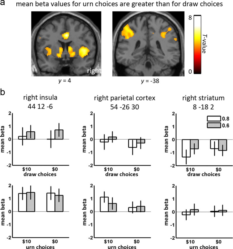
Urn choices versus draw choices contrast. a, Results of contrast urn choices > draw choices thresholded at p < 0.001 uncorrected, as observed in anterior cingulate, insula and striatum (left), and bilateral parietal cortex (right). b, Mean beta values and 90% confidence intervals at peak coordinates of areas in a, as a function of color probability and loss.

Figure 4.

Parietal cortex is associated with number of draw choices. a, Areas in right dorsolateral prefrontal cortex (left) and right parietal cortex (right) where beta values corresponding to urn choices showed positive linear relationships with average number of draws, thresholded at p < 0.001 uncorrected. b, Scatter plot of beta values for draw choices at the peak voxel in right parietal cortex, showing no positive associations with the number of draws. c, Scatter plot of beta values for urn choices for the same peak voxel, showing a positive association with the number of draws separately for all four conditions.

Figure 5.

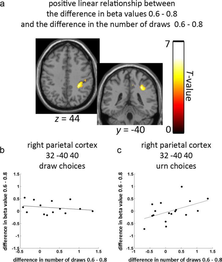
Parietal cortex was associated with the majority color probability behavioral effect. a, Area in right parietal cortex where individual differences in the beta value contrast 0.6 > 0.8 (effect of color probability) predicted corresponding differences in the number of draw choices (0.6 > 0.8), thresholded at p < 0.001. b, Scatter plot showing no relationship between the color probability fMRI contrast (beta values at the peak voxel in right parietal cortex) for draw choices and the size of the probability effect on the number of draws. c, Scatter plot showing a positive linear relationship between the probability fMRI contrast (beta values at the peak voxel in right parietal cortex) for urn choices and the size of the color probability effect on the number of draws.

Figure 6.

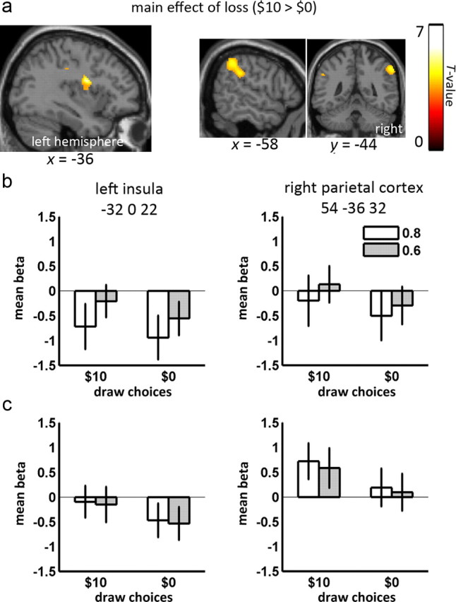
Main effect of loss. a, The beta value contrast $10 > $0 yielded two areas: left posterior insula (left) and right inferior parietal cortex (right), thresholded at p < 0.001 uncorrected. b, Beta values for draw choices are shown for left posterior insula (left) and right inferior parietal cortex (right). Bars show the mean beta values and error bars show the 90% confidence intervals. c, Mean beta values and 90% confidence intervals for urn choices are greater for $10 losses than $0 at peak voxels in left posterior insula (left) and right inferior parietal cortex (right).

Figure 7.

Parametric modulation of urn choice responses by model-based estimate of value of the chosen action. We fit a parameterized version of our Bayesian model to the choices of our participants and thereby derived model estimates of the value Q associated with each chosen action. These “action values” were then related statistically to the fMRI data. a, Urn choice responses in right posterior insula modulated by action values Q, thresholded at p < 0.001 uncorrected. These results derived from testing whether the mean across all four conditions differed from zero. b, Means and 90% confidence intervals for action value modulation (beta values) as a function of color probability and loss for bead events leading to draw choices (left) and urn choices (right).

Once we had computed the beta value (estimated BOLD response magnitude) for each of our events of interest, as well as contrasts over these beta values (see Results), we then brought these to a “second level” of analysis where they were entered into one-sample t tests, treating participants as a random effect. This allowed us to test whether beta values were statistically constant across participants. All results reported below were observed at p < 0.001 and then tested for familywise error (FWE) correction at the cluster level at P(FWE) < 0.05 using Gaussian random field theory. This is a conventional method (Brett et al., 2003; Friston et al., 2007) that uses the estimated smoothness of the data to correct for the massive number of multiple comparisons at all voxels in the whole brain.

Results

Behavioral results

Behavioral results from the scanning sessions are shown in Figure 2 and statistics are reported in Table 1. Figure 2 and Table 1 also show estimated optimal choices from our Bayesian ideal observer model. We computed these optimal choices by submitting to the ideal observer model the same bead sequences available to each of the 17 participants, including the extra beads that the participants could have drawn. The average ideal observer performance could thus be computed separately for the sequences specific to each participant. We can refer to the performance obtained from the ideal observer model that corresponded to a specific participant as “participant-matched ideal performance.” In this way, the ideal observer model could provide an estimate of what each individual participant should have chosen. Considering both the participants and their participant-matched ideal observer counterparts as comparable decision making agents, we could statistically contrast their decision making performance using an “agent type” factor.

Figure 2.

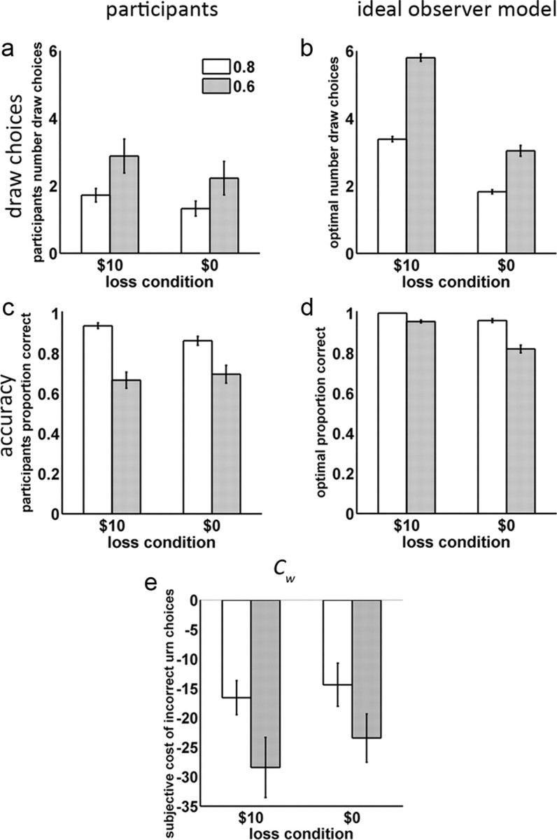
Behavioral performance as a function of color probability and loss. a, Mean and SE of the number of draws chosen by participants. b, Optimal number of draws derived from ideal observer. Although the same ideal observer model was always used to compute optimal performance for all sequences, we organized our results so that ideal observer performance scores could be separately matched to each participant's performance. These participant-matched scores were used to compute SEs (error bars) and statistical contrasts with participants. c, Mean and SE of the participants' accuracy. d, Optimal accuracy for ideal observer (SEs computed over participant-matched scores. e, The cost of incorrect urn choices C_w, estimated from participant behavior using parameterized Bayesian model.

Table 1.

Behavioral ANOVA results

Effect	Draws		Accuracy
	Participants	Ideal observer	Participants	Ideal observer
Probability	F(1,16) = 6.82, p = 0.02	F(1,16) = 336.16, p < 0.01	F(1,16) = 5.01, p = 0.01	F(1,16) = 97.83, p < 0.01
Loss	F(1,16) = 20.79, p < 0.01	F(1,16) = 515.86, p < 0.01	n.s.	F(1,16) = 58.96, p < 0.01
Probability × loss	n.s.	F(1,16) = 28.90, p < 0.01	F(1,16) = 4.54, p = 0.05	F(1,16) = 13.39, p < 0.01
Comparison of agent type (human vs ideal observer)
Agent type	F(1,16) = 50.84, p < 0.01		F(1,16) = 107.64, p < 0.01
Agent type × probability	F(1,16) = 24.84, p < 0.01		n.s.
Agent type × loss	n.s. p = 0.07		F(1,16) = 14.55, p < 0.01
Agent type × probability × loss	F(1,16) = 6.61, p = 0.02		F(1,16) = 18.64, p < 0.01

n.s., Not significant.

On the average, the ideal observer drew more beads than the participants (see Agent type main effect, Table 1, and compare Fig. 2a,b). Both the participants and ideal observer significantly increased the number of draws for 0.60 probability sequences, compared with 0.80 sequences. However, the ideal observer showed a significantly larger drawing increase than the participants (see Agent type × probability interaction, Table 1). This increased drawing led to increased accuracy for 0.60 sequences, compared with 0.80 sequences, for both the participants and the ideal observer (Fig. 2c,d). However, because the drawing increase was greater for the ideal observer, it showed a significantly larger accuracy increase than for the participants (see Agent type × probability interaction, Table 1). A similar pattern was observed for the loss conditions. Both the participants and the ideal observer increased the number of draws for $10 loss sequences, compared with $0 loss sequences, although the ideal observer showed a larger increase than the participants (see Agent type × loss interaction, Table 1). This increased drawing also significantly benefited accuracy in the $10 loss condition more for the ideal observer compared with the participants (see Agent type × loss interaction, Table 1). Last, the ideal observer disproportionately drew more beads when there was both a 0.60 probability and a potential $10 loss, while the participants did not. Consequently, the ideal observer showed a significant probability × loss interaction for draws while the participants did not and, moreover, there was a significant agent type × probability × loss interaction (Table 1). These interaction effects on the number of draws were accompanied by a corresponding agent type × probability × loss interaction effect on accuracy. In summary, the ideal observer drew more beads overall, and was more willing to increase drawing rates in response to low majority color probability or potential $10 losses. Consequently, the ideal observer benefitted more from its increased drawing with increased accuracy and therefore winnings.

We also examined our Bayesian model-based parameter estimates for the subjective cost of incorrect urn choices C_w. One participant was excluded as an extreme outlier (produced values of <−270, compare with Fig. 2e) and we further applied a log transformation to the data to satisfy ANOVA assumptions of normality for computation of the statistics. The pattern of C_w values paralleled that of accuracy and the number of draws. The absolute magnitude of C_w values was greater (more negative) for 0.6 than the 0.8 color probability conditions (F_(1,15) = 4.53, p = 0.05). Although numerically C_w values showed greater absolute magnitude in the $10 loss condition than that of $0, neither the loss main effect nor the value × loss interaction achieved significance.

fMRI responses associated with urn choices

We first contrasted the estimated size of the BOLD response (beta values) related to urn choices (bead presentations leading to decisions to name either the blue or green urn) to those related to draw choices (bead presentations leading to decisions to draw another bead). We chose this contrast to illustrate brain areas that were related to urn choices, controlling for irrelevant factors such as visual stimulation and motor execution that were common to both urn and draw choices. We identified a pattern of areas (Fig. 3, Table 2), all thought to contribute to decision making (see Introduction). This included a large cluster which encompassed the left parietal cortex, including the vicinity of intraparietal sulcus (IPS), left striatum and left insula (including parts of adjacent frontal cortex). Other clusters were observed in homologous areas of the right parietal cortex, also including the vicinity of inferior IPS, right striatum and right insula. Urn choices evoked larger BOLD responses (beta values) than draw choices also in anterior cingulate and a cluster encompassing substantia nigra and posterior thalamus. For completeness, we also tested the reverse contrast, draw choices > urn choices. This contrast revealed effects in visual cortex as well as several areas not predicted a priori including the superior frontal gyrus and temporoparietal junction (Table 2). We also observed posterior cingulate, an area previously implicated in exploratory behaviors in monkeys (Pearson et al., 2009).

Table 2.

Areas differentiating urn choices and draw choices

	Brodmann areas	MNIa			Size (2 mm3 voxels)	Peak t-value
Urn choices > draw choices
Right insula	13, 44, 45	44	12	−6	1751	8.03
Anterior cingulate	24, 32, 8, 9	4	4	38	1166	7.90
Left parietal cortex	40, 2, 7, 5	−58	−28	42	3817	7.80
Left insula	13, 47	−32	20	−16
Left putamen, caudate, globus pallidus		−14	10	−4
Thalamus, substantia nigra, red nucleus		8	−18	2	442	4.43
Right parietal cortex	40, 2	54	−26	30	1042	4.31
Right caudate, putamen		10	8	6	600	4.19
Draw choices > urn choices
Left superior frontal gyrus	6, 8	−20	32	58	337	7.87
Right visual cortex	18	20	−86	−10	384	4.42
Precuneus, posterior cingulate	7, 30, 29, 23, 30	−4	−50	4	839	6.59
Left superior frontal gyrus	6	−14	4	64	307	6.33
Left temporoparietal junction	39, 7	−50	−66	42	276	5.76

^aMNI coordinates x, y, z.

Areas correlated with behavioral measures

In the next series of analyses, we examined correlations between the estimated size of the BOLD response (beta values) related to urn choices and various behavioral measures. We first searched the whole brain for voxels which showed a significant linear relationship between beta values related to urn choices and individual differences in the participants' average number of draws. We found voxels that showed these significant effects within two areas (Fig. 4a): one in the right dorsolateral prefrontal cortex (peak MNI: 54 16 28, 186 voxels encompassing parts of Brodmann area 9 and 46) and one in the right parietal cortex (MNI: 40 −40 40, 261 voxels within Brodmann area 40). The right parietal area was near the lower bank of the IPS and overlapped with the right parietal area observed when we contrasted urn choices with draw choices (Fig. 3, Table 2). There was no significant correlation between the average number of draws and beta values for draw choices (Fig. 4b). For urn choices, we intended our correlation analysis (Fig. 4a) to identify areas that were correlated in common across all our conditions. To verify that our results were not driven by any subset of conditions (e.g., by only the 0.8 or 0.6 conditions), we also examined regressions separately for each individual condition. These correlations were not driven by any subsets of conditions, as we found robust linear effects in all conditions for both dorsolateral prefrontal and parietal cortex (See Fig. 4c, Table 3).

Table 3.

Relationships between beta values and the number of draws

	β	ρ	F(1,15)	P
Right dorsolateral prefrontal cortex (MNI:a 54 16 28)
Urn choice events
0.8/$10	0.96	0.53	5.78	0.03
0.6/$10	0.63	0.36	24.53	0.01
0.8/$10	1.25	0.72	28.26	<0.01
0.6/$10	0.67	0.44	16.29	<0.01
Draw choice events
0.8/$10	−0.01	−0.01	0.001	0.97b
0.6/$10	0.75	0.76	15.25	<0.01b
0.8/$10	0.38	0.30	0.85	0.38b
0.6/$10	0.52	0.82	9.42	<0.01b
Right parietal cortex (MNI: 40 −40 40)
Urn choice events
0.8/$10	1.02	0.63	10.04	<0.01
0.6/$10	0.48	0.43	33.36	<0.01
0.8/$10	1.12	0.61	22.15	0.01
0.6/$10	0.75	0.47	53.10	<0.01
Draw choice events
0.8/$10	0.26	0.23	0.64	0.44b
0.6/$10	0.09	0.48	0.67	0.43b
0.8/$10	−0.07	−0.30	0.02	0.88b
0.6/$10	0.16	0.10	1.57	0.23b

^aMNI coordinates x, y, z.

^bIncluded voxels failed to reach the thresholds necessary for significance in whole-brain analysis of either p < 0.001 uncorrected or P(FWE) < 0.05 cluster level.

Although parietal responses in each of the individual conditions in the design were related to behavioral disposition to draw, it is still possible that differences among conditions could relate to how much participants adjusted their drawing between these conditions. We thus tested whether the fMRI data related to differences in drawing between the levels of the color probability and loss factors. We found no correlations relating the fMRI data to differences in the number of draws for individual participants for the loss conditions ($10 > $0). Next, we examined the contrast 0.6 > 0.8 for beta values associated with urn choices. This contrast, when computed for every participant, represents the individual differences in the size of the majority color probability effect on beta values for urn choices. We found that the size of this contrast correlated positively with the corresponding behavioral effect on the number of draws (0.6 > 0.8) at voxels in right parietal cortex (MNI: 32 −40 40, 322 voxels within Brodmann area 40; Fig. 5). That is, participants who increased their evidence seeking in the 0.6 condition were also more likely to show larger beta values related to urn choices. This area was similar to that observed to be greater for urn choices than for draw draws. It was further similar to that correlated with each of the four draw conditions. That is, we observed all three parietal effects to be overlapping and nearby and inferior to IPS. We found no negative correlations nor did we find any corresponding correlations for draw choices (Fig. 5b).

Main effects of loss and color probability

In addition to regressions of behavioral measures on beta values related to urn choices, we also directly contrasted the beta values related to urn choices in the different task conditions. Beta values related to urn choices in the 0.6 condition did not differ from those in the 0.8 condition when averaged over participants. However, in Figure 6, we show that beta values for urn choices differed between the two loss conditions ($10 > $0) in the left posterior insula (MNI: −32 0 22, 475 voxels near Brodmann area 13) and right inferior parietal cortex (MNI: 54 −36 32, 577 voxels encompassing Brodmann areas 40, 3 and 2). This right inferior parietal area partially overlapped with the parietal areas described above; however, it is centered somewhat more inferiorly and is clearly inferior to the IPS.

Action values, surprise, conditional probability, and Bayesian confidence

At the first analysis level, for each participant's data, we parametrically modulated our draw choice and urn choice regressors using quantities related to the parameterized Bayesian ideal observer model (See Materials and Methods). To identify whether any brain areas were associated on a draw-by-draw basis with certainty, predictability or confidence, we ran three separate types of first-level models (See Materials and Methods). In the first type of model, our regressors were modulated by the conditional probability associated with the bead color revealed to the participant (blue or green). In the second type of model, our regressors were modulated by the corresponding quantity of surprise (the negative log₂ of the conditional probability of the bead produced by the draw). The third type of model used a measure of Bayesian confidence (See Materials and Methods). Neither conditional probability nor surprise produced any significant modulation when tested at the second, group level. Bayesian confidence showed greater modulation for draw choices than for urn choices in right low-level visual cortex (MNI: 12 −78 20 251 voxels peaking in Brodmann area 18). A more ventral area of the right occipital lobe showed greater modulation during draw choices for 0.8 sequences than for 0.6 sequences (MNI: 40 −84 −18, 395 voxels peaking in Brodmann area 18). This contrast also revealed an area in left frontal cortex (MNI: −42 0 56, 163 voxels peaking in Brodmann area 6). All three of these measures also functioned as nuisance variables (See Materials and Methods). Thus, the effects reported in Figures 3–7 cannot be simply accounted for by the increased predictability of the bead shown when an urn choice was made.

For every first-level analysis, we also parametrically modulated our regressors using the estimated action values Q, corresponding to the action chosen by the participant for each draw. We examined the parametric modulation of urn choices by Q at the group level (Fig. 7) by collapsing over the four conditions and testing whether their mean modulation differed from zero. We observed a significant effect in the right posterior insula (MNI: 30 −14 6, 398 voxels in Brodmann area 13). We also tested for a parametric modulation of draw choice events by the action values for draws but observed no effect.

Discussion

Using the beads task (Fig. 1), we investigated how people decide how much evidence to actively collect before acting in expectation of reward. Compared with a Bayesian ideal observer model, participants sought less evidence than optimal (Fig. 2). Also, under conditions when the ideal observer increased its optimal evidence seeking, participants increased their evidence seeking by a smaller amount. Participants' willingness or disposition to seek evidence (Fig. 4) and to adjust their evidence seeking (Fig. 5) was associated with BOLD responses evoked by urn choice events in parietal cortex. Also, responses in the insula covaried with the action values, or expected gains, of urn choices (Fig. 7). Together, these areas may be associated with decisions to terminate evidence-seeking.

Our participants appeared to treat evidence seeking as a costly activity and sought evidence sparingly, even at the expense of accuracy and monetary gain. Our ideal observer model chose to draw more than the participants and achieved higher accuracy and therefore more winnings. The ideal observer model also showed a larger increase in the number of draws than participants when the majority bead color probability was closer to chance (0.60), as opposed to when it was higher probability (0.80). When confronted with potential $10 losses, the ideal observer model also increased evidence seeking more and benefitted from a greater improvement in accuracy than the participants did. The participants' sparing evidence seeking appears suboptimal from a financial perspective, as the cost of drawing was small ($0.25), compared with the much larger amount ($10) available to win. Participants would thus have incurred little monetary cost to obtain larger winnings using higher drawing rates, as the ideal observer model did. The choices of this ideal observer model, though optimal, provide a limited description of participants' choices, as it considers only monetary outcomes. Our participants, in contrast, appeared to consider costs, aside from financial gain, that we did not include in our model. In naturalistic settings, evidence seeking can be a dangerous activity. It consumes time as well as biological and cognitive resources (e.g., working memory, attention, memory), whose limited availability also may place further time constraints. Humans may therefore be predisposed to minimize non-monetary costs such as these. Minimized evidence seeking behavior may have further consequences. Using a paradigm similar to the beads task, participants appear to underestimate the prevalence of low-probability events, a phenomenon attributed to reliance on small information samples derived from limited evidence-seeking (Hertwig and Erev, 2009).

The choice to seek additional evidence might be mediated via a neural mechanism which, like the Bayesian model, compares the costs of seeking additional evidence to the potential gains and losses of an immediate reward-related decision. This process can be modeled with a threshold mechanism, such that when the value of acting to obtain a reward exceeds the value of seeking additional evidence, the action is taken (e.g., See Materials and Methods for details of Bayesian model). Parietal cortex appears to be the best candidate suggested by our data for making this comparison. First, parietal cortex may play a role in generating an urn choice, as urn choices evoked larger beta values here than draw choices (Fig. 3) and no significantly positive beta values were observed for draw choices. The magnitude of the parietal BOLD response for urn choices further correlated with participants' disposition to draw (Fig. 4). In addition, parietal responses evoked by urn choices also correlated with participants' disposition to increase the amount of evidence seeking when necessary. Participants who drew more for 0.60 majority color sequences than for 0.80 majority color sequences showed a correlated response difference between these conditions in the right parietal cortex (Fig. 5). Last, parietal cortex was further associated with urn choices that, if incorrect, could potentially lead to $10 losses (Fig. 6). Thus, parietal cortex might relate to the increase in evidence seeking in the $10 condition, compared with the $0 condition. All these contrasts consistently revealed effects in the right parietal cortex, nearby and inferior to the right intraparietal sulcus. These results could be collectively explained if the parietal cortex estimated the value of continuing to perform evidence-seeking actions relative to the value of making a reward guided action.

These findings are incompatible with alternative accounts of parietal function. A number of studies concluded that parietal cortex communicates decision confidence (Kiani and Shadlen, 2009) or stimulus predictability (Huettel et al., 2005; Yang and Shadlen, 2007; Gläscher et al., 2010; Stern et al., 2010). There may indeed exist neurons in intraparietal sulcus that signal confidence (Kiani and Shadlen, 2009) although they likely reflect different populations of neurons than our findings. First, our parietal findings related to increased evidence seeking on the 0.60 condition. However, urn choices in the 0.6 condition were not likely to be more confident, as 0.6 condition draws conveyed less information and participants were less accurate. Second, the conditional probability, surprise or Bayesian confidence associated with each event was not associated with parietal cortex. Third, these regressors acted as nuisance covariates (see Materials and Methods and Results). Because beta values in a general linear model control for variation in the other regressors, all of the beta values we report in Figures 3–7 control for variability in the conditional probability, surprise and Bayesian confidence. In the context of the beads task, individual differences in the parietal BOLD responses related to how much evidence participants were willing to seek to support their final urn decision, rather than the confidence of the final decision or the predictability of the final event.

More alternative accounts may also be considered. First, drawing more beads may place greater demands on cognitive resources such as working memory and attention (Corbetta and Shulman, 2002). Second, participants may be counting bead colors and there is evidence that parietal cortex signals number magnitude (Piazza et al., 2007; Arsalidou and Taylor, 2011). These accounts all predict correlations between the number of draws and parietal responses to any bead draw, regardless of whether a draw choice or an urn choice was made. They cannot as easily explain how response correlations were found for responses to urn choices but not responses to draw choices.

Urn choices might be associated with parietal cortex because it participates in the final decision to select an urn. The absence of detectable parietal BOLD response for draw choices is surprising in light of prior studies that suggest that parietal cortex integrates evidence as it is collected (Huk and Shadlen, 2005; Kiani and Shadlen, 2009; Domenech and Dreher, 2010). Similarly, the explore/exploit paradigm has linked exploratory actions with parietal responses (Daw et al., 2006) and other areas including anterior cingulate (Hayden et al., 2011) and posterior cingulate (Pearson et al., 2009). Indeed, this last finding may relate to our result that posterior cingulate was associated with draw choices (Table 2). Explore/exploit and related paradigms (Behrens et al., 2007) differ from the beads task because outcomes from reward-related decisions can inform future reward-related decisions. The beads task uniquely addresses a specific question these other paradigms do not: how does an agent choose between unrewarded actions which function solely to collect evidence versus actions that, if properly informed, can be rewarded? The aforementioned paradigms do not explicitly require this choice, as agents in these paradigms always act to gain reward (or avoid punishment). We suspect therefore that our experimental context was necessary to reveal a population of neurons in parietal cortex that can be instrumental in choosing a final, reward-related action over an unrewarded evidence-seeking action.

Along with parietal cortex, the insula is prevalent in a wide range of decision making contexts including task difficulty, ambiguity and uncertainty (Heekeren et al., 2004; Huettel et al., 2005, 2006). Here, we found insula BOLD responses were greater for $10 than $0 losses (Fig. 7), consistent with previous studies showing that insula relates to potential losses (Venkatraman et al., 2009; Xue et al., 2010) and risky decisions (Mohr et al., 2010). Of relevance to our conclusions is the finding that insula responses were modulated by the action values, or expected gain of urn choices, as computed from our parameterized Bayesian model. This model predicts that evidence seeking ceases and a final urn choice made when the value of one of the urn choices exceeds the value of seeking more evidence. Following this model, it is possible that the termination of evidence seeking and the execution of a reward-related decision may have been mediated by a combination of the signals we observed in parietal cortex and insula, which, respectively, communicated the disposition to seek evidence and the value of urn choices.

In conclusion, participants were less inclined to seek evidence in the beads task than predicted by a Bayesian ideal observer model. Further, several lines of evidence linked parietal responses associated with reward-related decisions with participants' willingness to overtly act to seek evidence. The parietal cortex may be associated with the amount of evidence seeking chosen by the participant, while insula is associated with weighing the value of making an urn decision. Together, these two areas might support the minimization of the costs and risks associated with evidence seeking.

References

- Arsalidou M, Taylor MJ. Is 2 + 2 = 4? Meta-analyses of brain areas needed for numbers and calculations. Neuroimage. 2011;54:2382–2393. doi: 10.1016/j.neuroimage.2010.10.009. [DOI] [PubMed] [Google Scholar]
- Averbeck BB, Evans S, Chouhan V, Bristow E, Shergill SS. Probabilistic learning and inference in schizophrenia. Schizophr Res. 2011;127:115–122. doi: 10.1016/j.schres.2010.08.009. [DOI] [PMC free article] [PubMed] [Google Scholar]
- Basten U, Biele G, Heekeren HR, Fiebach CJ. How the brain integrates costs and benefits during decision making. Proc Natl Acad Sci U S A. 2010;107:21767–21772. doi: 10.1073/pnas.0908104107. [DOI] [PMC free article] [PubMed] [Google Scholar]
- Behrens TE, Woolrich MW, Walton ME, Rushworth MF. Learning the value of information in an uncertain world. Nat Neurosci. 2007;10:1214–1221. doi: 10.1038/nn1954. [DOI] [PubMed] [Google Scholar]
- Bertsekas D. Dynamic programming and optimal control. Belmont, MA: Athena Scientific; 1995. [Google Scholar]
- Brett M, Penny WD, Kiebel SJ. Introduction to random field theory. In: Frackowiak RSJ, Friston KJ, Frith C, Dolan R, KJ, Price CJ, Zeki S, Ashburner J, Penny WD, editors. Human brain function. Ed 2. San Diego: Academic; 2003. [Google Scholar]
- Cisek P, Puskas GA, El-Murr S. Decisions in changing conditions: the urgency-gating model. J Neurosci. 2009;29:11560–11571. doi: 10.1523/JNEUROSCI.1844-09.2009. [DOI] [PMC free article] [PubMed] [Google Scholar]
- Corbetta M, Shulman GL. Control of goal-directed and stimulus-driven attention in the brain. Nat Rev Neurosci. 2002;3:201–215. doi: 10.1038/nrn755. [DOI] [PubMed] [Google Scholar]
- Daw ND, O'Doherty JP, Dayan P, Seymour B, Dolan RJ. Cortical substrates for exploratory decisions in humans. Nature. 2006;441:876–879. doi: 10.1038/nature04766. [DOI] [PMC free article] [PubMed] [Google Scholar]
- Ding L, Gold JI. Caudate encodes multiple computations for perceptual decisions. J Neurosci. 2010;30:15747–15759. doi: 10.1523/JNEUROSCI.2894-10.2010. [DOI] [PMC free article] [PubMed] [Google Scholar]
- Domenech P, Dreher JC. Decision threshold modulation in the human brain. J Neurosci. 2010;30:14305–14317. doi: 10.1523/JNEUROSCI.2371-10.2010. [DOI] [PMC free article] [PubMed] [Google Scholar]
- Friston KJ, Fletcher P, Josephs O, Holmes A, Rugg MD, Turner R. Event-related fMRI: Characterizing differential responses. Neuroimage. 1998;7:30–40. doi: 10.1006/nimg.1997.0306. [DOI] [PubMed] [Google Scholar]
- Friston KJ, Ashburner JT, Kiebel SJ, Nichols TE, Penny WD. Statistical parametric mapping: the analysis of functional brain analysis. London: Academic; 2007. [Google Scholar]
- Gläscher J, Daw N, Dayan P, O'Doherty JP. States versus rewards: dissociable neural prediction error signals underlying model-based and model-free reinforcement learning. Neuron. 2010;66:585–595. doi: 10.1016/j.neuron.2010.04.016. [DOI] [PMC free article] [PubMed] [Google Scholar]
- Hayden BY, Pearson JM, Platt ML. Neuronal basis of sequential foraging decisions in a patchy environment. Nat Neurosci. 2011;14:933–939. doi: 10.1038/nn.2856. [DOI] [PMC free article] [PubMed] [Google Scholar]
- Heekeren HR, Marrett S, Bandettini PA, Ungerleider LG. A general mechanism for perceptual decision-making in the human brain. Nature. 2004;431:859–862. doi: 10.1038/nature02966. [DOI] [PubMed] [Google Scholar]
- Hertwig R, Erev I. The description-experience gap in risky choice. Trends Cogn Sci. 2009;13:517–523. doi: 10.1016/j.tics.2009.09.004. [DOI] [PubMed] [Google Scholar]
- Huettel SA, Song AW, McCarthy G. Decisions under uncertainty: probabilistic context influences activation of prefrontal and parietal cortices. J Neurosci. 2005;25:3304–3311. doi: 10.1523/JNEUROSCI.5070-04.2005. [DOI] [PMC free article] [PubMed] [Google Scholar]
- Huettel SA, Stowe CJ, Gordon EM, Warner BT, Platt ML. Neural signatures of economic preferences for risk and ambiguity. Neuron. 2006;49:765–775. doi: 10.1016/j.neuron.2006.01.024. [DOI] [PubMed] [Google Scholar]
- Huk AC, Shadlen MN. Neural activity in macaque parietal cortex reflects temporal integration of visual motion signals during perceptual decision making. J Neurosci. 2005;25:10420–10436. doi: 10.1523/JNEUROSCI.4684-04.2005. [DOI] [PMC free article] [PubMed] [Google Scholar]
- Huq SF, Garety PA, Hemsley DR. Probabilistic judgements in deluded and non-deluded subjects. Q J Exp Psychol A. 1988;40:801–812. doi: 10.1080/14640748808402300. [DOI] [PubMed] [Google Scholar]
- Ivanoff J, Branning P, Marois R. fMRI evidence for a dual process account of the speed-accuracy tradeoff in decision-making. PLoS One. 2008;3:e2635. doi: 10.1371/journal.pone.0002635. [DOI] [PMC free article] [PubMed] [Google Scholar]
- Kiani R, Shadlen MN. Representation of confidence associated with a decision by neurons in the parietal cortex. Science. 2009;324:759–764. doi: 10.1126/science.1169405. [DOI] [PMC free article] [PubMed] [Google Scholar]
- Mohr PN, Biele G, Heekeren HR. Neural processing of risk. J Neurosci. 2010;30:6613–6619. doi: 10.1523/JNEUROSCI.0003-10.2010. [DOI] [PMC free article] [PubMed] [Google Scholar]
- Pearson JM, Hayden BY, Raghavachari S, Platt ML. Neurons in posterior cingulate cortex signal exploratory decisions in a dynamic multi-option choice task. Curr Biol. 2009;19:1532–1537. doi: 10.1016/j.cub.2009.07.048. [DOI] [PMC free article] [PubMed] [Google Scholar]
- Piazza M, Pinel P, Le Bihan D, Dehaene S. A magnitude code common to numerosities and number symbols in human intraparietal cortex. Neuron. 2007;53:293–305. doi: 10.1016/j.neuron.2006.11.022. [DOI] [PubMed] [Google Scholar]
- Puterman M. Markov decision processes: discrete stochastic dynamic programming. New York: Wiley; 1994. [Google Scholar]
- Shadlen MN, Newsome WT. Neural basis of a perceptual decision in the parietal cortex (area LIP) of the rhesus monkey. J Neurophysiol. 2001;86:1916–1936. doi: 10.1152/jn.2001.86.4.1916. [DOI] [PubMed] [Google Scholar]
- Stern ER, Gonzalez R, Welsh RC, Taylor SF. Updating beliefs for a decision: neural correlates of uncertainty and underconfidence. J Neurosci. 2010;30:8032–8041. doi: 10.1523/JNEUROSCI.4729-09.2010. [DOI] [PMC free article] [PubMed] [Google Scholar]
- Venkatraman V, Rosati AG, Taren AA, Huettel SA. Resolving response, decision, and strategic control: evidence for a functional topography in dorsomedial prefrontal cortex. J Neurosci. 2009;29:13158–13164. doi: 10.1523/JNEUROSCI.2708-09.2009. [DOI] [PMC free article] [PubMed] [Google Scholar]
- Xue G, Lu Z, Levin IP, Bechara A. The impact of prior risk experiences on subsequent risky decision-making: the role of the insula. Neuroimage. 2010;50:709–716. doi: 10.1016/j.neuroimage.2009.12.097. [DOI] [PMC free article] [PubMed] [Google Scholar]
- Yang T, Shadlen MN. Probabilistic reasoning by neurons. Nature. 2007;447:1075–1080. doi: 10.1038/nature05852. [DOI] [PubMed] [Google Scholar]