Estimating the Reliability of Single-Item Life Satisfaction Measures: Results from Four National Panel Studies

Abstract

Life satisfaction is often assessed using single-item measures. However, estimating the reliability of these measures can be difficult because internal consistency coefficients cannot be calculated. Existing approaches use longitudinal data to isolate occasion-specific variance from variance that is either completely stable or variance that changes systematically over time. In these approaches, reliable occasion-specific variance is typically treated as measurement error, which would negatively bias reliability estimates. In the current studies, panel data and multivariate latent state-trait models are used to isolate reliable occasion-specific variance from random error and to estimate reliability for scores from single-item life satisfaction measures. Across four nationally representative panel studies with a combined sample size of over 68,000, reliability estimates increased by an average of 16% when the multivariate model was used instead of the more standard univariate longitudinal model.

1 Introduction

Assessing the reliability of a set of scores is a critical first step in all data analyses. Scores that have low reliability contain considerable amounts of error and are generally problematic for many research contexts. However, estimating the reliability of scores from single-item measures can be difficult, as commonly used indexes of internal consistency cannot be computed when there is only one item. Because single-item measures play an important role in research where respondent burden is a primary concern (for example in longitudinal studies or large-scale survey research), improving the estimation of reliability for scores from such measures is an important goal.

Typically, reliability is assessed using one of two techniques, each of which relies on different assumptions and each of which has distinct strengths and weaknesses (Alwin 2007; Biemer et al. 2009). The most common approach is to examine the internal consistency of the various items that make up a measure. Computing Cronbach’s alpha is the simplest version of this approach, though structural equation modeling techniques can also be used to estimate the amount of true-score variance that exists within a set of observed scores. These approaches typically assume that the individual items are at least parallel measures and that each item taps only a single underlying trait. If this assumption is violated and individual items contain reliable unique variance that is not shared with the underlying trait of interest, then internal-consistency-based techniques may underestimate the true reliability of the measure. In contrast, if items share reliable variance from more than one latent trait (for instance, if the items tapped a substantive trait factor and an independent method factor) or if errors for individual items are correlated, then this could lead to artificially high reliability estimates.

An alternative to this approach, and one that can be used with both single- and multiple-item measures, is to use longitudinal data to estimate reliability. For instance, with three or more waves, quasi-simplex models can be used to model an underlying latent trait with an autoregressive structure (see Alwin 2007, for a discussion). The proportion of total variance at each wave that is accounted for by this autoregressive trait can be used as an estimate of reliability. Like internal-consistency-based estimates, the quasi-simplex model makes certain assumptions. First, it assumes that the underlying trait has a first-order autoregressive structure. However, if the measures contain variance that is completely invariant across time in addition to variance that changes in predictable ways over time, then this approach will lead to artificially high stability estimates for the autoregressive trait. Because the observed wave-to-wave correlations will be smaller than expected based on the estimated stability of the autoregressive trait, the estimates of error variance can be positively biased. Fortunately, these concerns can be addressed by modeling a stable latent trait in addition to the autoregressive trait, as specified in Kenny and Zautra’s (1995, 2001) Stable Trait, Autoregressive Trait, State (STARTS) Model.

Second, simplex approaches assume that there is stationarity either in true-score or error variance (Biemer et al. 2009). In other words, the models assume that either the amount of true-score variance is constant across measurement occasions or the amount of error variance is constant across occasions. If either assumption is incorrect (and the wrong one is modeled), then reliability estimates will be biased. Recently, Biemer et al. (2009) proposed a Generalized Simplex model that addresses this limitation. By using split halves for multiple-item scale scores, this model can test the stationarity assumptions. In addition, correlated error variances within a single wave can be estimated to account for occasion specific sources of measurement error that are unrelated to the true score. Thus, assumptions underlying both the internal consistency and simplex-model approaches can be tested and the consequences of incorrect assumptions on reliability estimates can be assessed. Unfortunately, this model is not suitable for single-item measures because it requires a minimum of two indicators at each measurement occasion. In such cases the standard simplex model is recommended (Biemer et al. 2009).

A third assumption (and one that is most central to the current work) concerns occasion-specific variance. Both the Generalized Simplex model and the standard Simplex model assume that any variance that is unique to a single occasion is error variance. However, for many psychological constructs, the existence of occasion-specific true-score variance is a possibility, particularly if the interval between waves is long. Thus, reliability estimates that are derived from longitudinal models can be negatively biased if substantial amounts of occasion-specific but reliable variance exist. To address this issue, researchers have typically combined short- and long-term longitudinal studies (e.g., Ehrhardt et al. 2000; Schimmack et al. 2010), using an estimate of the short-term test–retest correlation to correct for the bias that results from the overestimate of error variance across longer intervals. Schimmack et al. also showed how multivariate longitudinal models can be used to address this issue. In such models, both a target measure and a correlate can be assessed and decomposed into stable trait, autoregressive trait, and transient state components. Then the correlations between the two sets of components can be estimated. If the state component for the target measure consists solely of random error, then it should not correlate with any other variable (by definition). If, however, this state component is significantly associated with the state component for the correlate, then this would suggest that reliable occasion-specific variance exists. The size of the association between the state components for the two constructs can provide a lower-bound estimate of this reliable occasion-specific variance in each construct.

We note at the outset that this approach assumes that variance that is shared across measures is variance that should be included in the estimate of true-score variance. It is certainly not random error, but such variance could also reflect some form of systematic occasion-specific factor that is unrelated to the true score, such as the effect of current mood. There are two reasons why we believe it is important to consider this source of potentially reliable variance. First, there is no strong a priori reason to assume that such variance reflects systematic error rather than true-score variance. Multi-method data would be required to determine whether it should be considered error or true-score variance, and such data are often not available. Yet all models must make some untested assumption about what to do with this type of variance. In the Generalized Simplex model, it is assumed that any occasion-specific covariance reflects systematic error. But this could just as easily reflect reliable and valid occasion-specific variance that does not carry over across waves. Second, the multivariate model we use in the current studies provide a method for testing the sensitivity of this assumption. When multi-method data are available, an alternative method of assessment can be used for the correlate, which would make it less likely that any covariance would reflect systematic error. In any case, because both assumptions are equally plausible, it is worth evaluating the effects that assumptions about occasion-specific variance have on reliability estimates in longitudinal contexts.

In the current study, we illustrate these issues by comparing the reliability of a single-item life satisfaction measure as estimated by (a) the standard STARTS model and (b) a multivariate STARTS model using aggregated domain satisfaction ratings as a correlate. These analyses are replicated across four nationally representative panel studies with a combined sample size of over 68,000 respondents.

2 Method

2.1 Participants and Measures

The German Socio-Economic Panel Study (GSOEP) is a nationally representative household panel study that began in 1984 (Haisken-De New and Frick 2005). We use the original West German sample, from which 24 waves of data are available (N = 13,155). Participants were surveyed yearly, some in face-to-face interviews, some with self-report questionnaires, and some with computerized testing. Life satisfaction was assessed with the item “All things considered, how satisfied are you with your life as a whole?” Responses were indicated using an 11-point scale ranging from 0 “totally dissatisfied” to 10 “totally satisfied.” Participants were also asked to rate their satisfaction with their health, their household income, their dwelling, and their leisure time. A few other domain satisfaction questions were asked in some waves or asked of some participants (e.g., job satisfaction was asked of those who were employed), but these are not included in the analyses. Participants used the same response options as with the general life satisfaction question.

The British Household Panel Study (BHPS) is a nationally representative panel study that began in 1991 (University of Essex, Institute for Social and Economic Research 2004; see Taylor et al. 2004, for more details). Eleven waves are available, and the total N = 26,176. Life satisfaction was assessed with the item “How dissatisfied or satisfied are you with your life overall?” Responses were indicated using a 7-point scale ranging from 1 “not satisfied at all” to 7 “completely satisfied.” Participants were also asked to rate their satisfaction with their health, household income, house/flat, social life, amount of leisure time, and use of their leisure time. Again, other questions were asked of some participants, but these are not included in the analyses. Participants used the same response options as with general life satisfaction.

The Household, Income, and Labour Dynamics in Australia Study (HILDA) is a nationally representative household panel study that began in 2001 (Watson 2010). Eight waves were available for these analyses, with a total sample size of 19,594. Life satisfaction was assessed with the item “All things considered, how satisfied are you with your life?” Responses were indicated using an 11-point scale ranging from 0 “totally dissatisfied” to 10 “totally satisfied.” Participants were also asked to rate their satisfaction with their health, their financial situation, the home in which they lived, their safety, the extent to which they felt a part of their community, their neighborhood, and the amount of leisure time time they had (and again other unanalyzed questions were asked of some participants). Participants used the same response options as with the general life satisfaction question.

The Swiss Household Panel Study (SHP) is a nationally representative household panel study that began in 1999 (life satisfaction assessment began in 2000). Surveys were conducted over the phone. We restrict our analyses to those individuals from the a sample that was recruited in 1999 and who have up to 8 waves of data (N = 9,112). Life satisfaction was assessed with the item “All things considered, how satisfied are you with your life as a whole?” Responses were indicated using an 11-point scale ranging from 0 “totally dissatisfied” to 10 “totally satisfied.” Participants were also asked to rate their satisfaction with their health, their financial situation, their free time, and their leisure activities (other questions were asked in some waves or of some participants, but these are not included in the analyses). Participants used the same response options as with the general life satisfaction question.

2.2 Analytic Technique

The STARTS model presented in Fig. 1 decomposes multi-wave data into three components: a stable trait component, an autoregressive trait component, and a state component. The model is equivalent to a simplex model with an added stable trait. Complete details of the model specification are reported in Kenny and Zautra (1995, 2001) and are briefly summarized here. The path from the latent stable trait to each observed measure is constrained to be 1.0. The path from each wave of the latent autoregressive trait to its corresponding observed measure is also constrained to be 1.0. Finally, the path from each latent state variable (which can also be thought of as the residual for the observed variable) to its corresponding observed measure is constrained to be 1.0. The variances for these three latent variables are estimated. In addition, the stability coefficient for the autoregressive component is estimated. The standard STARTS model imposes a stationarity assumption such that the variance components and stabilities are assumed to be the same across all waves. This is accomplished by constraining all parameters to be equal across waves (i.e., the autoregressive residual variance, state variance, and stability coefficients are constrained to be the same across waves).¹ In addition, the residual variance for the autoregressive component (U in Fig. 1) is constrained to be equal to the variance of the initial autoregressive component minus the product of this variance and the square of the stability. In this model, reliability is estimated to be the ratio of the sum of the stable trait and autoregressive trait variance to total variance. Alternatively, 1—minus the proportion of state variance in the construct provides the same estimate of the reliability of the scores in a given dataset.

Fig. 1.

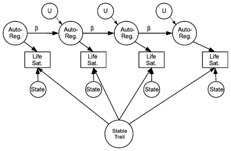
Diagram of the stable trait autoregressive trait state model

The bivariate STARTS model is a simple extension of the univariate model. Separate models are estimated for two constructs (Schimmack et al. 2010). The two stable-trait components, the two initial autoregressive-trait components, and autoregressive residual components from the same wave are allowed to correlate with one another (correlations between concurrent autoregressive residual components are constrained to be equal across waves). Finally, a new latent variable that reflects the variance that is shared between the state components for the target variable (life satisfaction in this case) and the correlate (domain satisfaction) is included. To identify the model in a bivariate context, the paths from this variable to the latent state variables are constrained to be equal to 1.0. As we discuss in the next section, this constraint can be relaxed with more than two variables. In addition, the variance of this new latent trait is constrained to be equal across all waves. In this multivariate model, the reliability of the measure is estimated to be the ratio of the sum of the stable trait, autoregressive trait, and shared state variance to the total variance. In other words, occasion-specific variance that is shared across constructs is included as part of the true-score variance when calculating reliability. The argument for this assumption is that state variance that correlates across constructs is not random error and therefore should not “count against” the cross-sectional reliability of the scores. Because there are missing data, full information maximum likelihood estimation is used for all models. All models were estimated in Mplus 5.21 (Muthén and Muthén 1998–2009).

3 Results

Table 1 presents fit indexes, variance decompositions, and reliability estimates for the univariate and bivariate models in each of the four samples. With the possible exception of the univariate model in the HILDA, the fit of the models was acceptable by current conventions (see e.g., Brown 2006, pp. 86–89) with CFIs and TLIs above 0.95, RMSEAs at or below 0.05, and SRMRs below 0.08. The variance decomposition columns report the percentage of variance accounted for by each of the components. We use the term “residual” to refer both to the state component in the univariate model (as this is technically the residual term for the observed variable) and to the residual term for the latent state factor in the multivariate model. Reliability is calculated as 1 minus the percentage of variance accounted for by this residual in each model.

Table 1.

Fit statistics and variance decompositions for the univariate and bivariate STARTS models

Study	Model	Fit statistics								Variance decomposition				Reliability	% Increase
		χ2	df	p	N	CFI	TLI	RMSEA	SRMR	Stable trait	Auto-regressive	Shared state	Residual
GSOEP
	Univariate	3868.661	296	0.000	13155	0.97	0.97	0.03	0.07	0.26	0.36		0.39	0.61
	Bivariate	8669.545	1164	0.000	13155	0.98	0.98	0.02	0.06	0.27	0.34	0.13	0.26	0.74	0.21
BHPS
	Univariate	471.576	62	0.000	26153	0.99	0.99	0.02	0.04	0.38	0.24		0.37	0.63
	Bivariate	1025.443	241	0.000	26176	1.00	1.00	0.01	0.03	0.37	0.25	0.11	0.26	0.74	0.17
HILDA
	Univariate	811.711	32	0.000	19592	0.98	0.98	0.04	0.10	0.31	0.32		0.37	0.63
	Bivariate	1594.386	124	0.000	19594	0.99	0.99	0.03	0.07	0.37	0.27	0.09	0.27	0.73	0.16
SHP
	Univariate	148.373	32	0.000	9109	0.99	0.99	0.02	0.04	0.26	0.36		0.38	0.62
	Bivariate	468.983	124	0.000	9112	0.99	0.99	0.02	0.03	0.34	0.28	0.05	0.32	0.68	0.09

Table 1 shows that the univariate models consistently estimate the reliability of the life satisfaction measure to be about 0.62. The multivariate models, however, generally show that there is a moderate amount of occasion-specific variance that is shared between constructs. If this variance is counted as true-score variance then there is a sizable increase in estimated reliability for single-item measures. For three of the four studies, the percentage of reliable variance increased by approximately 20% from the univariate models, with estimates of 0.74, 0.74, and 0.73 in the GSOEP, BHPS, and the HILDA. The estimate for the SHP was lower (0.68), but this still reflects a 9% increase in the amount of reliable variance in the measure.

4 Discussion

The estimation of reliability is a critical task in the analysis and interpretation of research (Thompson 2003). Researchers who use single-item measures are faced with unique challenges in this domain and longitudinal approaches would seem to be the most direct avenue for estimating reliability when single-item measures are used. However, standard longitudinal models assume that any occasion-specific variance is error variance, and this assumption may lead to biases in the estimation of reliability. In this paper we show how univariate and multivariate STARTS models can provide estimates of the reliability for single-item measures using different sets of assumptions. Our analyses showed that the increase in estimated reliability that occurs when researchers count systematic occasion specific variance as true score variance can be substantial. Across the four studies, estimated reliability increased by an average of 16% from the univariate to the bivariate model. In three out of four studies, estimates for this single-item measure crossed the frequently cited heuristic for minimally acceptable reliability of 0.70. Although we recognize that measures with reliabilities below 0.70 are useful for some purposes (and that measures with reliabilities above 0.70 can still be problematic), reviewers and editors may often rely on this 0.70 cutoff when evaluating results of studies that use measures that have moderate levels of reliability (see Lance et al. 2006 for a discussion for this rule of thumb).

It is important to acknowledge two limitations of our proposed technique. First, a correlate of the target measure must have been assessed to implement this approach. In the current analyses, we chose a variable that should theoretically be linked with the construct of interest. However, the correlate does not have to be as close to the original construct as domain satisfaction is to life satisfaction for the approach to be useful. For instance, to assess the reliability of self-reported health, one could test a multivariate STARTS model with a variety of other indicators of health including symptom reports or doctors visits. Although the association between each alternative measure and self-reported health may be moderate to small, this association could be used to isolate reliable occasion-specific variance in the target construct.

The second limitation is that we cannot be sure that the shared within-occasion variance is really true-score variance as opposed to systematic error. However, the model provides a general approach that can be used to test this possibility. If the correlate that is used to examine occasion-specific variance is assessed using an alternative method, then many sources of systematic error can be ruled out. Schimmack and Lucas (2010) used a similar model to estimate spousal similarity in the GSOEP. In their model, simultaneous STARTS models were estimated for life satisfaction scores from husbands and wives. Although Schimmack and Lucas did not emphasize this result, their analyses showed that correlations between husbands’ and wives’ state variance were moderate in size, ranging from 0.25 to 0.32 (as compared to 0.50 for the correlation between state components of life and domain satisfaction in the GSOEP in the current study). These two measures assess different constructs using different respondents, yet the moderate correlations suggest that at least some of the occasion-specific variance is in fact true-score variance that should not count against the reliability of the scores.

It is also important to note that in the bivariate model that we used in this paper, the covariance between the state components is directly interpreted as an index of the amount of reliable occasion-specific variance that exists in each measure. This is because the loadings of the state component on the shared latent trait are necessarily constrained to be equal to identify the model. If the state component for one construct was actually more reliable than the other, then this assumption could lead to upward biases in the reliability estimate for the measure whose scores had lower reliability. However, with additional correlates, this constraint can be relaxed and the assumption can be tested. To demonstrate, we split the domain satisfaction measure from the HILDA into two separate scales consisting of three items each and then re-estimated the three-variable model with life satisfaction and two halves of the domain satisfaction measure. This allowed us to free the loadings from the shared state variance to the state component of each construct. Even in this modified model, the estimated reliability of the life satisfaction scores dropped only from 0.73 to 0.72.

In closing, it is important to acknowledge that all approaches for assessing reliability involve assumptions. Therefore, unqualified statements about the reliability of a set of scores are usually not warranted. In this paper, we have shown how state-trait models can be used to quantify the impact that assumptions about occasion-specific variance have on reliability estimation in longitudinal contexts. Our results suggest that single-item measures of life satisfaction might be considerably more reliable than some approaches indicate. In addition to increasing confidence in research using these measures, the methods we outlined can be used evaluate the reliability of measures of other constructs including those based on composite scores. All told, both univariate and multivariate STARTS models may provide researchers with even more tools for judging the psychometric adequacy of their measures.

References

- Alwin DF. Margins of error: A study of reliability in survey measurement. New York: Wiley; 2007. [Google Scholar]
- Biemer PP, Christ SL, Wiesen CA. A general approach for estimating scale score reliability from panel survey data. Psychological Methods. 2009;14:400–412. doi: 10.1037/a0016618. [DOI] [PMC free article] [PubMed] [Google Scholar]
- Brown TA. Confirmatory factor analysis for applied research. New York: Guilford Press; 2006. [Google Scholar]
- Ehrhardt JJ, Saris WE, Veenhoven R. Stability of life-satisfaction over time: Analysis of change in ranks in a national population. Journal of Happiness Studies. 2000;1:177–205. doi: 10.1023/A:1010084410679. [DOI] [Google Scholar]
- Haisken-De New JP, Frick J. Desktop companion to the German Socio-Economic Panel Study (GSOEP) Berlin: DIW; 2005. [Google Scholar]
- Kenny DA, Zautra A. The trait-state-error model for multi-wave data. Journal of Consulting and Clinical Psychology. 1995;63:52–59. doi: 10.1037/0022-006X.63.1.52. [DOI] [PubMed] [Google Scholar]
- Kenny DA, Zautra A. The trait-state models for longitudinal data. In: Collins LM, Sayer AG, editors. New methods for the analysis of change. Washington, DC: American Psychological Association; 2001. pp. 243–263. [Google Scholar]
- Lance CE, Butts MM, Michels LC. The sources of four commonly reported cutoff criteria: What did they really say? Organizational Research Methods. 2006;9:202–220. doi: 10.1177/1094428105284919. [DOI] [Google Scholar]
- Muthén LK, Muthén BO. Mplus user’s guide. 5. Los Angeles, CA: Muthén & Muthén; 1998–2009. [Google Scholar]
- Schimmack U, Lucas RE. Environmental influences on well-being: A dyadic latent panel analysis of spousal similarity. Social Indicators Research. 2010;98:1–21. [Google Scholar]
- Schimmack U, Wagner GG, Krause P, Schupp J. Stability and change of well being: An experimentally enhanced latent state-trait-error analysis. Social Indicators Research. 2010;95:19–31. [Google Scholar]
- Taylor MF, Brice J, Buck N, Prentice-Lane E. British Household Panel Survey user manual volume A: Introduction, technical report, and appendices. Colchester: University of Essex; 2004. Available at: http://iserwww.essex.ac.uk/ulsc/bhps/doc/ [Google Scholar]
- Thompson B, editor. Score reliability: Contemporary thinking on reliability issues. Thousand Oaks, CA: Sage; 2003. [Google Scholar]
- University of Essex. Institute for Social and Economic Research. British Household Panel Survey; waves 1–12, 1991–2003 [computer file] Colchester, Essex: UK Data Archive [distributor]; 2004. [Google Scholar]
- Watson N. HILDA user manual—release 8. Melbourne Institute of Applied Economic and Social Research, University of Melbourne; 2010. [Google Scholar]