

Abstract
Shrinkage of empirical Bayes estimates (EBEs) of posterior individual parameters in mixed-effects models has been shown to obscure the apparent correlations among random effects and relationships between random effects and covariates. Empirical quantification equations have been widely used for population pharmacokinetic/pharmacodynamic models. The objectives of this manuscript were (1) to compare the empirical equations with theoretically derived equations, (2) to investigate and confirm the influencing factor on shrinkage, and (3) to evaluate the impact of shrinkage on estimation errors of EBEs using Monte Carlo simulations. A mathematical derivation was first provided for the shrinkage in nonlinear mixed effects model. Using a linear mixed model, the simulation results demonstrated that the shrinkage estimated from the empirical equations matched those based on the theoretically derived equations. Simulations with a two-compartment pharmacokinetic model verified that shrinkage has a reversed relationship with the relative ratio of interindividual variability to residual variability. Fewer numbers of observations per subject were associated with higher amount of shrinkage, consistent with findings from previous research. The influence of sampling times appeared to be larger when fewer PK samples were collected for each individual. As expected, sample size has very limited impact on shrinkage of the PK parameters of the two-compartment model. Assessment of estimation error suggested an average 1:1 relationship between shrinkage and median estimation error of EBEs.
Electronic supplementary material
The online version of this article (doi:10.1208/s12248-012-9407-9) contains supplementary material, which is available to authorized users.
Key words: empirical Bayes estimate, mixed-effects models, population PK/PD, shrinkage
INTRODUCTION
The knowledge obtained from exposure–response modeling can facilitate the drug development process, and may be used to optimize patient response within the therapeutic window. Longitudinal data for drug exposure (i.e., drug concentrations) and pharmacological responses are often collected in a large number of subjects to understand the underlying relationship between pharmacokinetics (PK) and pharmacodynamics (PD) of a therapeutic agent. Mixed-effects modeling remains a popular tool for analyzing longitudinal PK or/and PD data (1–3). In population PK/PD analysis, individual parameter estimates, a combination of fixed and random effects, are often used as model diagnostic tools and subsequent individual-based analysis (4). Such estimations of individual parameters are usually referred to as empirical Bayes “estimates” (EBE) (5,6).
The distributions of EBEs obtained from mixed-effects models are usually narrower than those assumed to characterize the random variables being estimated. This type of phenomenon is called shrinkage in the Bayesian literature because subject-specific estimations are shrunk toward an appropriate population mean (7,8). However, there is some concern of the potential drawbacks of this phenomenon. Savic and Karlsson pointed out that the presence of a high level of shrinkage may compromise the usefulness of EBE-based diagnostic tools for mixed-effects models (4). Shrinkage may obscure the apparent correlations between random effects and covariate relationships or falsely induce such relationships (4,5). Overshrinkage can also lead to reduction in sensitivity to identify “extreme” individuals (9–11).
The amount of shrinkage has been shown to be associated with the quality of EBE-based model diagnostics (4). Empirical equations based on variability (i.e., standard deviation (SD) or variance) of estimated individual random effects were proposed to quantify the overall shrinkage of a parameter for a study population (4,12–14). Shrinkage has been studied extensively for mixed-effects models in statistical literature (15,16). Since different definitions and equations have been used and reported in PK/PD and statistical arenas, it is of great interest to compare the shrinkage calculation based on the proposed empirical equations in the PK/PD literature to that based on the theoretically derived equation in statistical literature. This may help to understand the similarity and differences between these shrinkage estimation equations and to avoid confusions.
As noted previously, shrinkage can lead to poor estimation of subject-specific random effects, particularly for subjects who exhibit much higher or lower values of parameters compared to the population mean (11). However, in a clinical study, those subjects who have extremely low or high drug exposure are usually at risk of being undertreated or experiencing unwanted adverse events. Therefore, understanding the impact of shrinkage on estimation error of subject-specific model parameters is important for exposure response analysis.
Although the focus of Savic and Karlsson’s work was on the impact of shrinkage on EBE-based diagnostics, it also suggested that the number of samples, sampling times, and residual errors are important factors affecting the overall shrinkage (4). However, some of the simulations in their work are ordinary simulations with a very small number of simulation replicates (i.e., n ≤ 10), therefore limiting the interpretation of the simulation results. Single ordinary simulations were carried out to evaluate some factors (i.e., magnitude of interindividual variability and residual variability, number of samples per subject, and estimation algorithm) that may influence the amount of shrinkage for clearance of a pharmacokinetic model (17). In this work, we first provided a theoretical derivation of shrinkage for a nonlinear mixed-effects model based on linear approximations as it has not been shown in the current literature. Also, we conduct Monte Carlo simulations (1) to compare commonly used shrinkage equations in a simple linear mixed-effects model, (2) to explore potential factors that may influence shrinkage for a pharmacokinetic model, and (3) to investigate the impact of shrinkage on the estimation error of posterior individual parameters.
METHODS
Random-Effects Estimation and Shrinkage in Nonlinear Mixed-Effects Models
In this section, we discuss and demonstrate the shrinkage of posterior individual random effects in a nonlinear mixed-effects model. Consider a non-linear mixed-effects model:
 |
1 |
where  , is a vector of observed response (e.g., drug concentration) for the ith subject who has ni observations, Xi is a covariate matrix for the ith subject (e.g., time), ηi is a q × 1 vector for the random effects and θ is a p × 1 vector of fixed effect. We assume that ηi ∼ N(0,Ω) and the residual error, εi ∼ N(0, Σi), and ηi and εi are independent of each other. Ω=Ω(θ,ϕ) and Σi=Σi(θ,φ) are the covariance matrices for the interindividual random effects and residual variability, respectively, where ϕ,φ are vector of parameters characterizing the covariance structures. By making first-order Taylor expansion of f(Xi,θ,ηi) at ηi = 0:
 |
2 |
where
 |
therefore,
 |
3 |
where Zi is known as the design matrix (ni × q), which links the random effects ηi to Yi, and contains the information for covariates including time invariant or/and time-varying covariates (15).
Similar to the derivations of shrinkage in linear mixed-effects models (15,16), by considering ηi,εij jointly follows a multivariate normal distribution  , we can obtain:
 |
therefore, ηi can be derived as
 |
The predicted response profile  can be then re-expressed as follows:
 |
4 |
where the weight (Wi) is the fraction of interindividual variability (IIV) from the overall variability:
 |
5 |
As it was shown in Eq. 4, the predictions of individual response profiles can be viewed as a weighted average of the population mean profile  and the observed data (Yi). The shrinkage in nonlinear mixed-effects models can be expressed as the weight associated with population mean as follows:
 |
6 |
Wi and SHi are computed at the estimated parameter values. When the residual variability  is large compared to the IIV, the shrinkage becomes large, whereas when IIV is greater than the residual variability, the shrinkage is small. This clearly demonstrates that the empirical Bayesian estimator shrinks the ith subject’s predicted response profile towards the population mean. It is noted that the derivation of Eq. 4 was based on the FO approximation (18–20). Similar derivations may also be made for other approximation algorithms such as the “first-order conditional” approach (known as FOCE) (21–24). However, due to the complexity and involvement of iterations in the FOCE algorithm, the derivation based on FOCE is not provided in this manuscript.
Variance functions are often used to model the heteroscedasticity of variance structure (Σi) of the residual errors. A general variance function model can be defined as (25,26):
 |
where νij is a vector of variance covariates, δ is a vector of variance parameters, and g(·) is the variance function. For the commonly used proportional and combined error structures, the variance models can be expressed as:
 |
Simulation Studies
Comparison of shrinkage equations for a linear mixed model
The purpose of this simulation was to compare the theoretically derived shrinkage equation (Eq. 6) with the empirical shrinkage equations commonly used in PK/PD research. Although Eq. 6 appears straightforward, the exact analytical solutions of shrinkage for nonlinear mixed-effects models are usually complex. However, the amount of shrinkage for some linear mixed-effects models can be readily quantified by simple equations. For the comparison purpose, a simple random intercept linear model was used for the simulation as follows:
 |
where ηi ∼ N(0, ω2), and εij ∼ N(0, σ2) with mutual independence.
For the random intercept model, Zi in Eq. 6 is an ni x1 vector of 1 s, and it can be shown that the theoretically derived shrinkage based on variance can be expressed using the following formula:
 |
7a |
Another intuitive way to calculate the shrinkage for the random intercept model can be based on the square root of the derived weight (SD of the variance):
 |
7b |
Empirical equations based on variability (i.e., SD or variance) of estimated individual random effects was used to quantify the shrinkage of the random intercept (4,13,14):
 |
8a |
 |
8b |
where  is the posterior estimate for individuals based on EBE and
  is the estimated standard deviation for the corresponding random effect.
For the random intercept linear model, Eq. 7a can be viewed as the derived counterpart of the variance version of the empirical shrinkage equation (Eq. 8a), while Eq. 7b is the derived counterpart for the SD version of the empirical shrinkage (Eq. 8b), which has been built into software like NONMEM and PsN (27,28). It should be noted that the SD-based shrinkage equations are just a function of the variance-based shrinkage equations, and can be easily converted to each other numerically.
The simulations were performed at low (≤15%), medium (45–65%), and high (≥90%) shrinkage levels (calculated based on Eq. 7a) for two different sampling schemes: one with six samples per subject and the other with 12 samples per subject. One hundred subjects were simulated for each trial, and the simulation was repeated 1,000 times. To simplify the simulation, all subjects in a trial have the same number of observations (either six or 12 samples per subject). The details of the simulations are described in Table I.
-
Simulation 2:
Factors Influencing Shrinkage in a PK Model
Table I.
Descriptions of Simulations Conducted to Evaluate the Empirical Shrinkage Equations Using a Linear Random-Intercept Model
| Simulation scenario | Number of observations | Interindividual variability | Residual variability | Shrinkage (%)a | Level of shrinkageb |
|---|---|---|---|---|---|
| 1 | 12 | 0.4 | 0.33 | 5.3 | Low |
| 2 | 12 | 0.3 | 1 | 48.1 | Medium |
| 3 | 12 | 0.01 | 4 | 97.1 | High |
| 4 | 6 | 0.4 | 0.33 | 10.2 | Low |
| 5 | 6 | 0.3 | 1 | 64.9 | Medium |
| 6 | 6 | 0.01 | 4 | 98.5 | High |
aCalculated based on the derived variance-based shrinkage equation (Eq. 7a) and the predefined values for the interindividual and residual variability used for simulations
bThe level of shrinkage is defined as follows: Low (≤15%); Medium (45–65%); and High (≥90%)
As Eq. 6 indicates, the amount of shrinkage is a function of the relative magnitude of interindividual and residual variability, the number of observations per subject, and the sampling times for the subject. The purpose of the simulations was to confirm how these factors affect the shrinkage of the parameters of a PK model. In addition, the impact of sample size was also investigated in the simulation study. Based on the theoretically derived shrinkage equation (Eq. 6), the sample size will not have an impact on the estimated shrinkage values. The purpose of the simulation for different sample size was simply to confirm the derived equation, and evaluate the impact of sample size on shrinkage estimation due to its influence on the precision of population estimates. It should be noted that the fixed-effect parameters were first estimated and the individual random effects were estimated subsequently by fixing the population parameters to their estimated values. Therefore, effects on both population parameter estimation and on shrinkage were studied. A two-compartment PK model with first-order oral absorption and first-order elimination was used for the simulations. The PK parameter values are listed in Table II. The random effects of the PK model were assumed to follow a log-normal distribution. An exponential residual error model was used to simulate the PK data. Due to involvement of wide range of factors, it is not practical to examine all the combinations of different values of these factors, and therefore only limited simulations were conducted to evaluate the impact of them. A number of simulation scenarios were considered for the four influencing factors on shrinkage as follows:
To evaluate the impact of the relative magnitude of inter- and intraindividual variability, the simulations were conducted with 12 PK samples for each subject at two IIV levels: 10% and 40%. For each IIV level, four levels of residual variability were investigated (10%, 20%, 40%, and 80%)
- To evaluate the impact of sampling times and number of observations, the inter- and intraindividual variabilities were fixed at 40% and 10%, respectively. The number of PK samples per subject was set to be two, four, eight, or twelve. For each of the two-, four-, and eight-sample scenario, four different sets of sampling times in hours were considered:
- (0.25, 24), (0.5, 20), (2, 16), and (4, 12)
- (0.25, 1, 16, 24), (0.5, 2, 12, 20), (1, 4, 8, 12), (2, 4, 6, 8)
- (0.25, 0.5, 1, 2, 12, 16, 20, and 24), (0.5, 1, 2, 4, 10, 12, 16, and 20), (1, 2, 4, 6, 8, 10, 12, and 16), and (0.5, 2, 4, 6, 8, 12, 18, and 24)
Table II.
PK Parameters Used for Simulation 2
| PK parameters | Population mean | Interindividual variability |
|---|---|---|
| CL (L/h) | 30 | 10% or 40%a |
| Vc (L) | 70 | 10% or 40%a |
| Vp (L) | 200 | 10% or 40%a |
| Q (L/h) | 20 | 10% or 40%a |
| KA | 1.5 | 10% or 40%a |
| Residual error | 10–80% (CV%)b |
CL clearance, Vc central volume of distribution, Vp peripheral volume of distribution, Q inter-compartmental clearance, KA absorption rate constant, CV coefficient of variation
aEither 10% or 40% was used for each simulation
bEither 10%, 20%, 40%, or 80% was used depending on the purpose of the simulation
Only one sampling time scenario was investigated for the case with 12 observations per subject, 0.25, 0.5, 1, 2, 4, 6, 8, 10, 12, 16, 20, and 24 h. The sampling times were selected arbitrarily. However, it is expected that samples at earlier times contains more information for absorption.
-
3.
To evaluate the impact of sample size, the inter- and intraindividual variabilities were fixed at 10% and 40%, respectively. Two levels of numbers of observations per subject (four and twelve) were studied. A sample size of 50, 100, 200, and 300 subjects per study was simulated and compared. For the four-sample simulation scenarios, PK samples were collected at 0.25, 1, 16, and 24 h
For each simulation, 100 PK datasets were simulated using NONMEM VI 2.0 [5]. One hundred subjects were included in each simulated dataset except for the simulation series that evaluates the impact of sample size. For each simulated trial, the same design was used for all subjects. The simulated dependent variable was log-transformed before modeling. The first-order conditional estimation method was used.
Impact of Shrinkage on Estimation of Individual PK Parameters
Due to the shrinkage feature of the estimated posterior Bayesian individual parameters, the performance and the quality of the Bayes estimator may be compromised. For a PK parameter, the relative deviation of an individual EBE for a subject from its corresponding true value being used for the simulation was evaluated by calculating the relative estimation error (REE%) as follows:
 |
where  is the true η value for the ith subject used for the simulation and
  is the posterior parameter estimate for that subject based on EBE. Median REE% was then calculated for each simulation trial to facilitate the comparison with the study-specific shrinkage. Median was used as the statistics to summarize the estimation error as it may be more suitable for situations where a normal distribution may not be applicable (29,30). Due to the shrinkage, the distribution of EBEs may not be normal. It is worth mentioning that the median of prediction errors has been utilized in PK/PD research as a model validation criterion (31,32). The calculated shrinkage amounts and median REE% percentages from all the simulations conducted in the Simulation 2 section were pooled and plotted against each other to evaluate the relationship between amount of shrinkage and degree of estimation error for individual PK parameters.
RESULTS
Comparison of Shrinkage Equations in a Linear Mixed Model
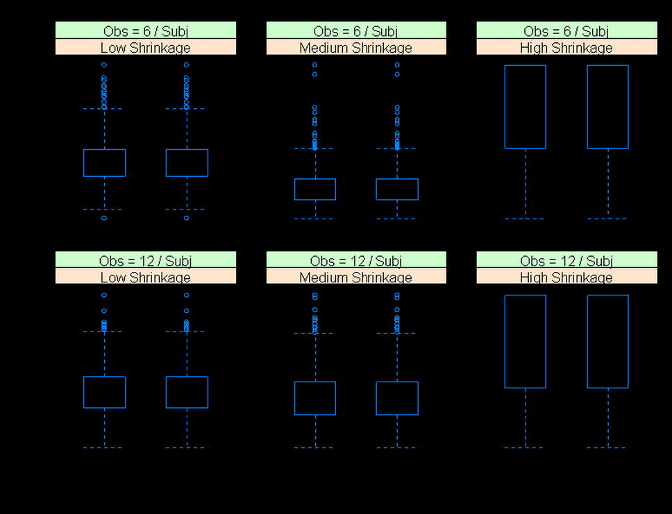
Figure 1 compares shrinkage values estimated from the variance-based derived and empirical shrinkage equations for the linear random intercept model for six different simulation scenarios described in Table I. The comparison for the SD-based derived and empirical shrinkage equations is presented in Supplementary Figure 1. The model estimated interindividual and residual variability were used for the estimation of shrinkage. The shrinkage values calculated from the derived shrinkage equations are almost identical to those based on the empirical shrinkage equations (Fig. 1). A closer examination of the shrinkage estimates from individual simulation replications found that the relative difference between the derived and the empirical equations was less than 0.0001%, suggesting that the simple empirical shrinkage equations could provide shrinkage estimates matching the values calculated based on theoretically derived equations. The variance-based empirical shrinkage was used in the later part of the manuscript (simulations for the two-compartment PK model) as its direct reflection of the weight for estimating individual response or parameters can be advantageous (Eq. 4).
Fig. 1.
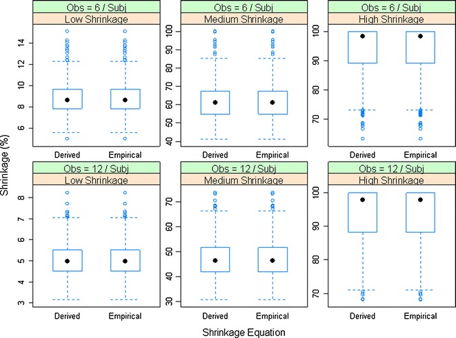
Comparison of the variance-based derived and empirical shrinkage equations for a linear random-intercept model. Model-estimated interindividual and residual variability were used in the equations
Evaluation of Influencing Factors on the Amount of Shrinkage
Since similar trend was observed for all the PK parameters, only the results for the primary PK parameters (i.e., CL and Vc) are discussed in the manuscript and are presented in the figures (Figs. 2, 3, 4, and 5), while the results for all the other PK parameters are provided in Supplementary Figures (Supplementary Figures 2–5).
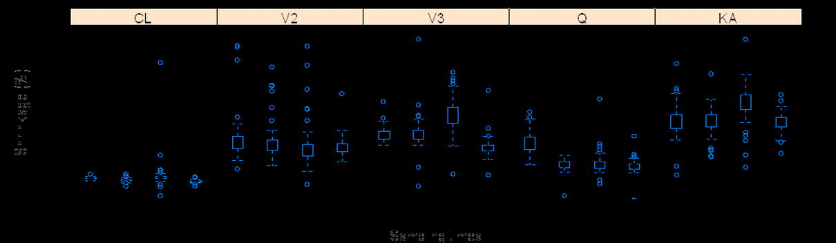
Fig. 2.
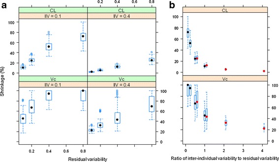
The relationship between shrinkage and residual variability at IIV = 10% and 40% for CL and Vc (a) and the relationship between shrinkage and ratio of interindividual variability to residual variability (b); in b, the boxplots with black and red median dots represent simulations for IIV = 10% and 40%, respectively. The empirical variance-based shrinkage was used
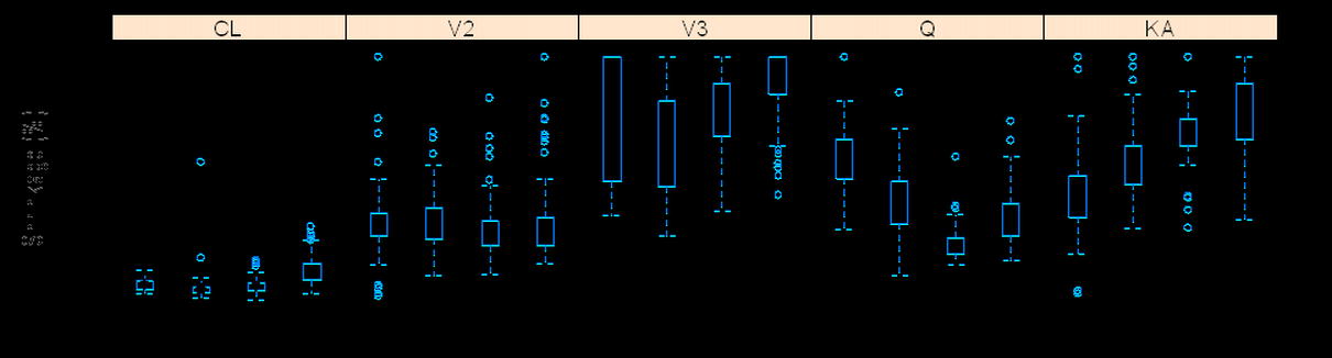
Fig. 3.
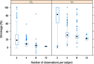
The relationship between shrinkage (empirical variance-based) and number of observations per subject for CL and Vc
Fig. 4.
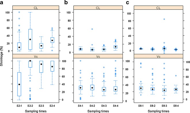
The influence of sampling times (in hours) on shrinkage of CL and Vc when observations per subject are two (a), four (b), or eight (c). S2-1: (0.25, 24), S2-2: (0.5, 20), S2-3: (2, 16), and S2-4: (4, 12); S4-1: (0.25, 1, 16, 24), S4-2: (0.5, 2, 12, 20), S4-3: (1, 4, 8, 12), and S4-4: (2, 4, 6, 8); and S8-1: (0.25, 0.5, 1, 2, 12, 16, 20, 24), S8-2: (0.5, 1, 2, 4, 10, 12, 16, 20), S8-3: (1, 2, 4, 6, 8, 10, 12, 16), and S8-4: (0.5, 2, 4, 6, 8, 12, 18, 24)
Fig. 5.
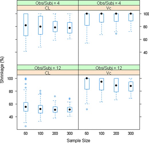
The relationship between shrinkage (empirical variance-based) and sample size for CL and Vc
Magnitude of Interindividual and Residual Variability
The influence of the magnitude of interindividual and residual variability on the shrinkage of posterior individual CL and Vc is shown in Fig. 2. At both levels of IIV (10% and 40%), as the residual variability increased, the shrinkage of the EBEs for the PK parameters increased until it reached a plateau around 100%. The amount of shrinkage at the 40% IIV level is generally lower than that at the 10% level. The CL appears to have lower shrinkage of the posterior individual estimates than the other PK parameters in the two-compartment model. Figure 2b demonstrates that as the ratio of IIV to residual variability increased, the shrinkage of the PK parameters decreased. In addition, it is also apparent that regardless of the absolute level of IIV and residual variability, when the ratio of IIV to residual variability is the same, the amount of shrinkage of EBEs for a PK parameter is similar, supporting that shrinkage is a function of the relative magnitude of IIV versus residual variability in non-linear mixed-effects models as Eq. 6 suggests.
Number of Observations and Sampling Times
As expected, lower shrinkage was clearly associated with larger numbers of observations per subject (Fig. 3). Under the current simulation conditions (40% IIV and 10% residual variability), when the number of observations per subject increased from two to 12, the median shrinkage of CL of the two-compartment model decreased from about 20% to <5%, while for Vc, the median shrinkage decreased from approximately 80% to about 20%. The smaller number of observations per subject was also related to a wider distribution of shrinkage values as the amount of shrinkage for both CL and Vc ranged from nearly 0% to 100% when there were only two PK samples per subject. This indicates that locations of sampling times may play a large role on estimation of posterior individual PK parameters and its associated shrinkage when the number of observations per subject is small. This is intuitively sensible because PK samples at different time points may carry different PK information. With fewer PK samples per subject collected, it is more important to design the PK sampling at optimized time points. In addition, when the number of observations is small, high imprecision in the population parameter estimates is expected, hence leading to more variability in the shrinkage. We further investigated the impact of sampling time points on the shrinkage by simulating four different sets of time points for each of the two, four, and eight observations per subject scenarios (Fig. 4). It appears that with two samples per subject, the variation in shrinkage across different sampling schemes was much higher than that with the four or eight samples per subject. The shrinkage of CL and Vc was very similar among different sampling schemes if four or eight PK samples were collected from each subject. This pattern was particularly apparent when there were eight observations per subjects. In the case of four samples per subject, as the early sampling points changed from 0.25 and 1 h to 2 and 4 h, the shrinkage on the EBEs of KA clearly increased from approximately 40% to nearly 80% (Supplementary Figure 4b). This makes sense because the information regarding the absorption phase mainly resides in the samples collected during early time points (0–2 h).
Sample Size
Sample size has very limited impact on shrinkage of the PK parameters (Fig. 5). The shrinkage of EBEs of CL appears to be smaller with a sample size greater than 100 compared to a sample size of 50. When the observations per subject were set to 12, the shrinkage of Vc EBEs appeared to be smaller at larger sample size. Theoretically, the sample size should not have an impact on the estimated shrinkage values. It is worth noting that a large sample size may help to reduce the variability in population parameter estimates and therefore to improve the precision of the estimation of shrinkage as a tighter distribution of shrinkage estimates across simulations can be observed when the sample size is larger. The small difference in median shrinkage values may be a result of larger variation in shrinkage at smaller sample size.
Relationship Between Shrinkage and Estimation Error
A scatter plot of the median estimation error of individual posterior η values of the PK parameters for each simulation dataset against the shrinkage calculated for that dataset is presented in Fig. 6. All the simulated PK datasets were combined to evaluate the relationship between shrinkage and estimation error of EBEs. An apparent linear relationship between the median estimation errors and the level of shrinkage was noted although some noise is present. Linear regression of the data for each PK parameter shows the slope is close to 1, suggesting there is 1:1 relationship on average between shrinkage and median estimation error of EBEs, i.e., a 40% shrinkage of a model/dataset means 40% estimation error of the individual-specific η values.
Fig. 6.
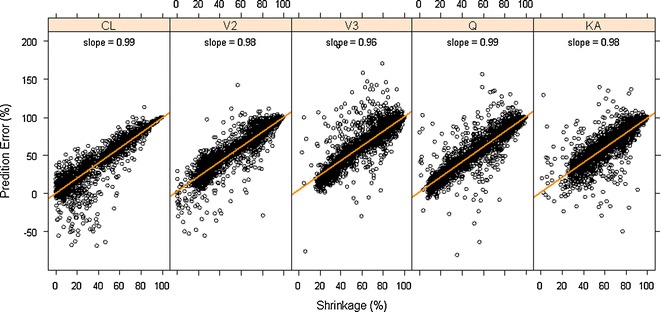
Impact of shrinkage (empirical variance-based) on median estimation error of subject-level parameter values for different PK parameters
DISCUSSION
The empirical Bayesian estimator is widely accepted for estimating posterior random effects for individuals (33). The tradeoff of this approach, as we mentioned previously and demonstrated in this manuscript, is its tendency to shrink estimates toward a population mean, which could lead to poor performance of the EB estimator, particularly in extreme regions of the random-effects distribution.
Shrinkage has become a popular indicator of the quality of the model building and evaluation procedure for population PK/PD models (4). Intuitive empirical shrinkage equations are commonly used for estimating overall shrinkage for population PK and PD models and datasets (4,13). Based on the theoretical derivations in this manuscript for nonlinear mixed models (Eq. 4) and in previous literature for linear mixed-effects models (15,16), posterior predicted responses for individuals can be viewed as weighted averages of population mean and observed data. Also, this weighting scheme can be also extended to estimate the EBEs of the individual parameters in linear models (15), where the EBEs of parameters  are expressed as linear combinations of the population mean value of a parameter
  and ordinary least square estimate
  based only on the individual’s observations with shrinkage as the weight as follows:
 |
9 |
where Iq is a q × q identity matrix, Ai is a design matrix including a set of between-individual covariates (a q × p matrix), and, again, Iq − Wi represents the shrinkage. Therefore, shrinkage can be interpreted and defined based on the theoretically derived weight. The simulations based on a linear model showed that the empirical shrinkage estimates were virtually same as the derived weight-based shrinkage. This result may provide a theoretical basis for the empirical equations, although they are already very intuitive as EBEs usually exhibit less variability than actually present in the population of random effects, ηi. It is worth mentioning that the variance-based shrinkage directly reflects the weights that can be used for predicting individual response profiles or posterior individual parameters, and therefore might be a natural choice for quantifying shrinkage. Further simulations are needed to investigate these shrinkage equations in nonlinear mixed-effects models, where such investigation is currently hampered by the lack of closed-form solutions of shrinkage.
The empirical shrinkage equations characterize the overall population shrinkage of a model and the underlying data. However, based on Eqs. 6, 7a, and 7b, shrinkage is indeed a subject-specific concept. Although the population shrinkage estimate may provide an indication of the overall performance of a model/dataset, it does not provide a means to resolve the problems caused by large shrinkage. Individual-level shrinkage has been proposed to choose informative EBEs which may serve as a basis for refined EBE-based diagnostics (34). As we noticed from the simulation study, the amount of shrinkage for the EBEs of a particular subject is dependent on the data quality (experimental errors), informativeness of samples (appropriateness of sampling times), and number of observations for that subject. Since population PK/PD often involve multiple studies and large numbers of subjects, a large amount of shrinkage may be encountered for such analysis due to poor data quality from poor sampling design, misconduct of a study or/and sparse data from late clinical phase studies. In such cases, an individual-based shrinkage estimation may allow identification and omission of influential individuals with inflated shrinkage from the EBE-based diagnostic plots (e.g., covariate search based on EBEs), and thereby reduce the impact of shrinkage on such diagnostic tools.
Since multiple factors (relative magnitude of IIV and residual error, sampling times, and number of observations per subject, etc.) may affect the shrinkage, appropriately interpreting and understanding the sources of shrinkage of a model parameter is important. When IIV is small (e.g., <10% IIV) and relatively big residual error (e.g., 30%), it can be expected that shrinkage may be large in this case as the relative magnitude of residual error is large. In this case, the large shrinkage toward the population mean is intuitive as the population is relatively homogeneous, and does not suggest a problematic model or less informative data but rather a homogeneous population. In situations where there is a high observed IIV (e.g., 20–30%), combined with a high residual error (40–50%), a large amount of shrinkage could indicate inappropriateness of a model (i.e., a poor choice of structural model) or large experimental errors (sampling errors or measurement errors). In this case, diagnostic plots on residual errors should be carefully examined to identify means to reduce the residual error. It is worth mentioning that shrinkage is only a secondary phenomenon and not as informative as residual error when it comes to model misspecification. When both IIV and residual error are within normal limits, a large shrinkage may indicate insufficient or non-informative data (small number of observations per subject or a poorly designed sampling scheme). It should be noted that lack of information (e.g., fewer observations and less informative sampling times) may also result in large standard errors of estimated population parameters in addition to high shrinkage of EBEs of random effects. Therefore, it is interesting to study the relationship between shrinkage of EBEs and standard errors of fixed- and random-effects parameters in future research.
To date, the discussion of the impact of shrinkage has been primarily focusing on model diagnostics and covariate model development using EBE-based random effects. Our research suggests that shrinkage of random effects can also be viewed as a metric of estimation error of posterior individual parameters. On average, there is an almost 1:1 relationship between the amount of shrinkage and the median relative estimation error for individual parameters. This means that high shrinkage of PK parameters could have profound impact on PK/PD analysis, particularly for sequential PK/PD analysis due to the use of posterior individual parameters in the approach. Since the amount of shrinkage varies among different PK parameters as was shown previously (4) and in the present simulation analysis, modelers need to evaluate and understand the amount of shrinkage for each PK parameter before choosing an appropriate PK measure (e.g., AUC, Cmin, or Cmax) for a sequential PK/PD analysis when summary PK variables are used. It appears that CL is usually the most well-informed PK parameter, and its EBEs are often associated with lower shrinkage (4). Therefore, AUC would be expected to be the most well-informed exposure variable. The influence of shrinkage should be limited for simultaneous PK/PD modeling. Some variations of sequential PK/PD methods (e.g., IPPSE and PPP&D) may reduce the influence of the shrinkage on estimation of PD parameters (35,36). In addition, various approaches, including nonparametric mixed-effects modeling and constrained Bayes estimation, have been proposed to reduce shrinkage in mixed-effects models (10,37,38). However, those topics are out of the scope of this article.
Savic and Karlsson suggested that a higher than 20–30% shrinkage (SD based) may result in misleading modeling diagnostics using EBEs (4). This amount of shrinkage is equivalent to approximately 40–50% shrinkage based on the variance-based shrinkage equation. This is intuitively sensible since shrinkage can be interpreted as the relative contribution to the estimation of individual parameters from either population mean estimates or individual OLS estimates (Eq. 9). When the shrinkage is greater than 50%, more contribution (weight) is provided by the population mean values, while the individual OLS estimates (or information from individuals) become more important when shrinkage is less than 50%. It can be expected that the correlations between random effects and covariate relationships may be falsely identified if EBEs of a parameter only contain limited information from individuals. The data from the current simulation study showed that the false-positive correlation between PK parameters increased with shrinkage (Supplementary Figure 6), confirming the previous findings (4). In addition, the cutoff value of 20–30% SD-based shrinkage may also be translated into approximately 50% estimation error in individual posterior model parameters.
In summary, the intuitive empirical shrinkage equations may provide shrinkage estimates close to those based on the theoretically derived equations for linear mixed-effects model. Further assessment is needed for nonlinear mixed models, particularly for population PK/PD models. The variance-based shrinkage directly reflects the weights that can be used for predicting individual response profiles or posterior individual parameters. In modeling practice, caution should be used to interpret the sources of shrinkage as multiple factors (e.g., relative magnitude of IIV and residual error, sampling times, and number of observations per subject, etc.) may affect the shrinkage. The present research suggests that, on average, there is a 1:1 relationship between the amount of shrinkage and the median relative estimation error for EBEs of PK parameters. Therefore, shrinkage can also be viewed as a metric of estimation error of posterior individual parameters. In addition, individual-based shrinkage may facilitate identification of subjects with inflated shrinkage and reduction of the influence of these subjects on EBE-based diagnostics.
Electronic Supplementary Material
Below is the link to the electronic supplementary material.
Comparison of the SD-based derived and empirical shrinkage equations for a linear random-intercept model. Model-estimated interindividual and residual variability were used in the equations (JPEG 56 kb)
The relationship between shrinkage (empirical variance based) and residual variability at IIV = 10% and 40% for different PK parameters (a) and the relationship between shrinkage and ratio of interindividual variability to residual variability (b); the boxplots with black and red median dots represent simulations for IIV = 10% and 40%, respectively (JPEG 59 kb)
The relationship between shrinkage (empirical variance based) and number of observations per subject for different PK parameters (JPEG 34 kb)
The influence of sampling times on shrinkage of PK parameters when observations per subject are two (a), four (b), or eight (c). S2-1: (0.25, 24), S2-2: (0.5, 20), S2-3: (2, 16), and S2-4: (4, 12); S4-1: (0.25, 1, 16, 24), S4-2: (0.5, 2, 12, 20), S4-3: (1, 4, 8, 12), and S4-4: (2, 4, 6, 8); and S8-1: (0.25, 0.5, 1, 2, 12, 16, 20, 24), S8-2: (0.5, 1, 2, 4, 10, 12, 16, 20), S8-3: (1, 2, 4, 6, 8, 10, 12, 16), and S8-4: (0.5, 2, 4, 6, 8, 12, 18, 24) (JPEG 32 kb)
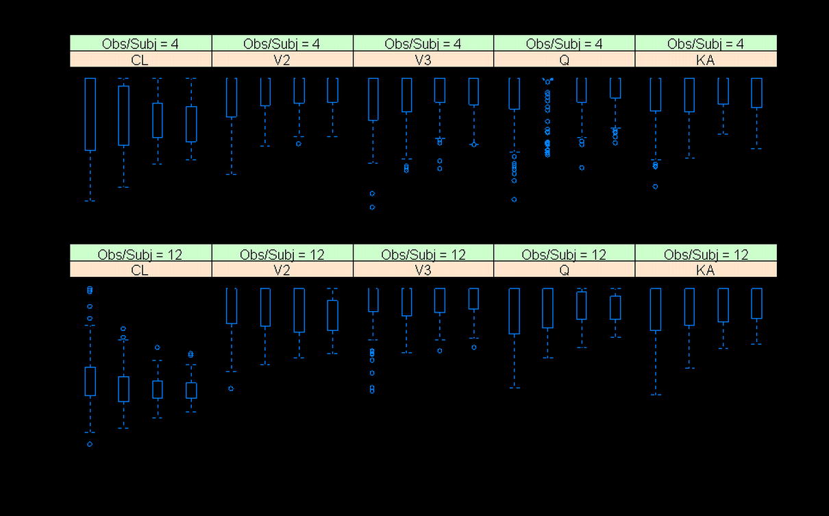
The relationship between shrinkage (empirical variance based) and sample size for different PK parameters (JPEG 69 kb)
The relationship between falsely induced correlation between η CL and η Vc and the shrinkage (empirical variance based) of the EBE estimates of the PK parameters. The 3D surface was constructed using LOWESS smoother. The true correlation between η CL and η Vc in the PK model was zero (JPEG 19 kb)
ACKNOWLEDGMENTS
There is no conflict of interest. Steven Xu is an adjunct assistant professor in the School of Public Health at the University of Medicine and Dentistry of New Jersey. This work is partially supported by the National Science Foundation of China (NSFC), Grant no. 11201452.
REFERENCES
- 1.Kloft C, Poggesi I. Current and future directions of pharmacokinetic and pharmacokinetic–pharmacodynamic modelling and simulation: population approach group in Europe 19th annual meeting. Expert Opin Drug Metab Toxicol. 2010;6(12):1599–1604. doi: 10.1517/17425255.2010.529899. [DOI] [PubMed] [Google Scholar]
- 2.Laird NM, Ware JH. Random-effects models for longitudinal data. Biometrics. 1982;38(4):963–974. doi: 10.2307/2529876. [DOI] [PubMed] [Google Scholar]
- 3.Sheiner L, Wakefield J. Population modelling in drug development. Stat Methods Med Res. 1999;8(3):183–193. doi: 10.1191/096228099672920676. [DOI] [PubMed] [Google Scholar]
- 4.Savic RM, Karlsson MO. Importance of shrinkage in empirical Bayes estimates for diagnostics: problems and solutions. AAPS J. 2009;11(3):558–569. doi: 10.1208/s12248-009-9133-0. [DOI] [PMC free article] [PubMed] [Google Scholar]
- 5.Fitzmaurice GM. Longitudinal data analysis. Boca Raton: Chapman & Hall; 2008. [Google Scholar]
- 6.Carlin BP, Louis TA. Bayesian methods for data analysis. 3. Boca Raton: CRC Press; 2009. [Google Scholar]
- 7.Carlin BP, Louis TA. Bayes and empirical Bayes methods for data analysis. 2. Boca Raton: Chapman & Hall; 2000. [Google Scholar]
- 8.Strenio JF, Weisberg HI, Bryk AS. Empirical Bayes estimation of individual growth-curve parameters and their relationship to covariates. Biometrics. 1983;39(1):71–86. doi: 10.2307/2530808. [DOI] [PubMed] [Google Scholar]
- 9.Louis TA. Estimating a population of parameter values using Bayes and empirical Bayes methods. J Am Stat Assoc. 1984;79:393–398. doi: 10.1080/01621459.1984.10478062. [DOI] [Google Scholar]
- 10.Ghosh M. Constrained Bayes estimation with applications. J Am Stat Assoc. 1992;87:533–540. doi: 10.1080/01621459.1992.10475236. [DOI] [Google Scholar]
- 11.Efron B, Morris C. Limiting the risk of Bayes and empirical Bayes estimators—part I: the Bayes case. J Am Stat Assoc. 1971;66:807–815. [Google Scholar]
- 12.Karlsson MO, Savic RM. Diagnosing model diagnostics. Clin Pharmacol Ther. 2007;82(1):17–20. doi: 10.1038/sj.clpt.6100241. [DOI] [PubMed] [Google Scholar]
- 13.Bertrand J, Comets E, Laffont CM, Chenel M, Mentre F. Pharmacogenetics and population pharmacokinetics: impact of the design on three tests using the SAEM algorithm. J Pharmacokinet Pharmacodyn. 2009;36(4):317–339. doi: 10.1007/s10928-009-9124-x. [DOI] [PMC free article] [PubMed] [Google Scholar]
- 14.INRIA (Institut National de la Recherche en Informatique et Automatique). Monolix 4.0.1 user Guide (http://www.lixoft.net/wp-content/uploads/2011/10/Monolix4-UserGuide1.pdf); 2011.
- 15.Fitzmaurice GM, Laird NM, Ware JH. Applied longitudinal analysis. Hoboken: Wiley-Interscience; 2004. [Google Scholar]
- 16.Verbeke G, Molenberghs G. Linear mixed models for longitudinal data. New York: Springer; 2000. [Google Scholar]
- 17.Bonate PL, SpringerLink (Online service). Pharmacokinetic–pharmacodynamic modeling and simulation. In. Boston, MA: Springer Science + Business Media, Inc.; 2006.
- 18.Sheiner LB, Beal SL. Evaluation of methods for estimating population pharmacokinetic parameters. III. Monoexponential model: routine clinical pharmacokinetic data. J Pharmacokinet Biopharm. 1983;11(3):303–319. doi: 10.1007/BF01061870. [DOI] [PubMed] [Google Scholar]
- 19.Sheiner BL, Beal SL. Evaluation of methods for estimating population pharmacokinetic parameters. II. Biexponential model and experimental pharmacokinetic data. J Pharmacokinet Biopharm. 1981;9(5):635–651. doi: 10.1007/BF01061030. [DOI] [PubMed] [Google Scholar]
- 20.Sheiner LB, Beal SL. Evaluation of methods for estimating population pharmacokinetics parameters. I. Michaelis–Menten model: routine clinical pharmacokinetic data. J Pharmacokinet Biopharm. 1980;8(6):553–571. doi: 10.1007/BF01060053. [DOI] [PubMed] [Google Scholar]
- 21.Vonesh EF. A note on the use of Laplace’s approximation for non-linear mixed-effects models. Biometrika. 1996;83:447–452. doi: 10.1093/biomet/83.2.447. [DOI] [Google Scholar]
- 22.Wolfinger RD. Laplace’s approximation for non-linear mixed models. Biometrika. 1993;80:791–795. doi: 10.1093/biomet/80.4.791. [DOI] [Google Scholar]
- 23.Wolfinger RD, Lin X. Two Taylor-series approximation methods for nonlinear mixed models. Comput Stat Data Anal. 1997;25(4):465–490. doi: 10.1016/S0167-9473(97)00012-1. [DOI] [Google Scholar]
- 24.Lindstrom ML, Bates DM. Nonlinear mixed effects models for repeated measures data. Biometrics. 1990;46(3):673–687. doi: 10.2307/2532087. [DOI] [PubMed] [Google Scholar]
- 25.Davidian M, Giltinan DM. Nonlinear models for repeated measurement data. 1. London: Chapman & Hall; 1995. [Google Scholar]
- 26.Pinheiro JC, Bates DM, ebrary Inc . Mixed-effects models in S and S-PLUS. New York: Springer; 2000. [Google Scholar]
- 27.Lindbom L, Pihlgren P, Jonsson EN. PsN-Toolkit—a collection of computer intensive statistical methods for non-linear mixed effect modeling using NONMEM. Comput Methods Programs Biomed. 2005;79(3):241–257. doi: 10.1016/j.cmpb.2005.04.005. [DOI] [PubMed] [Google Scholar]
- 28.Bauer RJ. Nonmem users guide: introduction to Nonmem 7. Ellicott City: ICON Development Solutions; 2010. [Google Scholar]
- 29.Pfanzagl J, Hamböker R. Parametric statistical theory. W. de Gruyter, Berlin 1994.
- 30.van der Vaart HR. Some extensions of the idea of bias. Ann Math Stat. 1961;32(2):436–447. doi: 10.1214/aoms/1177705051. [DOI] [Google Scholar]
- 31.Sheiner LB, Beal SL. Some suggestions for measuring predictive performance. J Pharmacokinet Biopharm. 1981;9(4):503–512. doi: 10.1007/BF01060893. [DOI] [PubMed] [Google Scholar]
- 32.Bruno R, Vivier N, Vergniol JC, De Phillips SL, Montay G, Sheiner LB. A population pharmacokinetic model for docetaxel (Taxotere): model building and validation. J Pharmacokinet Biopharm. 1996;24(2):153–172. doi: 10.1007/BF02353487. [DOI] [PubMed] [Google Scholar]
- 33.Searle SR, Casella G, McCulloch CE. Variance components. New York: Wiley; 1992. [Google Scholar]
- 34.Savic R, Wilkins JJ, Karlsson MO. (Un)informativeness of empirical Bayes estimate-based diagnostics [abstr T3360]. AAPS J. 2006 8(S2).
- 35.Lacroix BD, Friberg LE, Karlsson MO. Evaluating the IPPSE method for PKPD analysis [Abstr 1843]. PAGE 2010;19:<www.page-meeting.org/?abstract=1843>.
- 36.Wade JR, Karlsson MO. Combining PK and PD data during population PK/PD analysis [Abstr 139]. PAGE 1999;8:<www.page-meeting.org/?abstract=139>.
- 37.Lyles RH, Xu J. Classifying individuals based on predictors of random effects. Multicenter AIDS Cohort Study. Stat Med. 1999;18(1):35–52. doi: 10.1002/(SICI)1097-0258(19990115)18:1<35::AID-SIM995>3.0.CO;2-#. [DOI] [PubMed] [Google Scholar]
- 38.Davidian M, Gallant AR. Smooth nonparametric maximum likelihood estimation for population pharmacokinetics, with application to quinidine. J Pharmacokinet Biopharm. 1992;20(5):529–556. doi: 10.1007/BF01061470. [DOI] [PubMed] [Google Scholar]
Associated Data
This section collects any data citations, data availability statements, or supplementary materials included in this article.
Supplementary Materials
Comparison of the SD-based derived and empirical shrinkage equations for a linear random-intercept model. Model-estimated interindividual and residual variability were used in the equations (JPEG 56 kb)
The relationship between shrinkage (empirical variance based) and residual variability at IIV = 10% and 40% for different PK parameters (a) and the relationship between shrinkage and ratio of interindividual variability to residual variability (b); the boxplots with black and red median dots represent simulations for IIV = 10% and 40%, respectively (JPEG 59 kb)
The relationship between shrinkage (empirical variance based) and number of observations per subject for different PK parameters (JPEG 34 kb)
The influence of sampling times on shrinkage of PK parameters when observations per subject are two (a), four (b), or eight (c). S2-1: (0.25, 24), S2-2: (0.5, 20), S2-3: (2, 16), and S2-4: (4, 12); S4-1: (0.25, 1, 16, 24), S4-2: (0.5, 2, 12, 20), S4-3: (1, 4, 8, 12), and S4-4: (2, 4, 6, 8); and S8-1: (0.25, 0.5, 1, 2, 12, 16, 20, 24), S8-2: (0.5, 1, 2, 4, 10, 12, 16, 20), S8-3: (1, 2, 4, 6, 8, 10, 12, 16), and S8-4: (0.5, 2, 4, 6, 8, 12, 18, 24) (JPEG 32 kb)
The relationship between shrinkage (empirical variance based) and sample size for different PK parameters (JPEG 69 kb)
The relationship between falsely induced correlation between η CL and η Vc and the shrinkage (empirical variance based) of the EBE estimates of the PK parameters. The 3D surface was constructed using LOWESS smoother. The true correlation between η CL and η Vc in the PK model was zero (JPEG 19 kb)