Abstract
In many eusocial Hymenoptera, a proportion of males are produced by workers. To assess the effect of male production by workers on the effective population size Ne, a general expression of Ne in Hymenoptera with worker-produced males is derived on the basis of the genetic drift in the frequency of a neutral allele. Stochastic simulation verifies that the obtained expression gives a good prediction of Ne under a wide range of conditions. Numerical computation with the expression indicates that worker reproduction generally reduces Ne. The reduction can be serious in populations with a unity or female-biased breeding sex ratio. Worker reproduction may increase Ne in populations with a male-biased breeding sex ratio, only if each laying worker produce a small number of males and the difference of male progeny number among workers is not large. Worker reproduction could be an important cause of the generally lower genetic variation found in Hymenoptera, through its effect on Ne.
Keywords: effective population size, Hymenoptera, worker-produced males
Introduction
Effective population size Ne is a crucial parameter in population, conservation and quantitative genetics, because this parameter determines both the rate of inbreeding and the amount of genetic drift in populations (Caballero, 1994; Falconer and Mackay, 1996; Frankham et al., 2002). In haplodiploid species, Ne has been predicted by applying Wright's (1933) standard formula for X-linked locus,
 |
where Nf and Nm are the numbers of breeding females and males, respectively. This application is reasonable, as inheritance in haplodiploid species is effectively equivalent to sex-linked inheritance in diploid species (Yokoyama and Nei, 1979; Page and Marks, 1982).
Colonies of eusocial Hymenoptera are characterized by a reproductive division of labour. Colonies are founded by mated females (queens), who produce diploid daughters (workers and young queens) and haploid males. Workers do not mate, but they retain ovaries in many species. If workers are sterile, only queens should be counted as the breeding females in the computation of Ne. Furthermore, under monogamous mating system as in many Hymenopteran species, both the numbers of queens and males are approximated by the number of nests, giving from equation (1) an estimate of Ne as the number of nests multiplied by 1.5 (Ellis et al., 2006). In some species, as honey bees and army ants, a queen mates with more than one male, leading to a biased breeding sex ratio (r=Nm/Nf) from unity. In such species, assuming the absence of worker reproduction, Ne has been predicted from equation (1) as
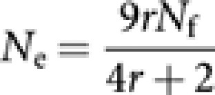 |
(Page and Marks, 1982). When r is large as in honey bees, 9Nf/4, that is, the number of nests multiplied by 9/4, can be a good approximation of Ne (Page and Marks, 1982).
It is, however, known that under certain conditions, workers lay unfertilized eggs which develop into males (Crozier and Pamilo, 1996). This production of males by workers is widespread in the eusocial Hymenoptera, such as stingless bees, honey bees, bumble bees, vespine wasps and higher ants (Crozier and Pamilo, 1996). Worker reproduction has received much attention in the context of evolution of sociality and altruism. For example, the kin selection theory of Hamilton (1964) predicts that haplodiploidy and its consequent asymmetric relationship among colony members cause a conflict over male production between queens and workers (Trivers and Hare, 1976; Queller et al., 1997). The conflict will be intensively expressed in a monogamous colony, because the workers should prefer to rear their own sons and nephews over their brothers (queen-produced males). This conflict has motivated many researchers to carry out theoretical and experimental studies (for example, Brown et al., 2003; Tsuchida et al., 2003; Wenseleers et al., 2004). In many species, worker-laid eggs are killed (policed) by the queen or by other workers. The policing is an important mechanism for resolving the queen–worker conflict and maintaining social harmony (Wenseleers et al., 2004), and also provides a clue for solving a question whether worker altruism is voluntary or enforced (Wenseleers and Ratnieks, 2006).
As for the effect of worker reproduction on Ne, there are two contrasting views. Contel and Kerr (1976) considered that the presence of worker-produced males will increase Ne because of the increased number of ‘genetically active' females. In contrast, Crozier and Pamilo (1996) predicted that worker reproduction decreases Ne, despite there being more breeding females, because an extra round of gametic sampling is introduced in each generation and the rate of genetic drift is enhanced. Owen and Owen (1989) derived an expression of Ne for the simplest case where each laying worker contributes exactly one breeding male. By numerical analysis with the obtained expression, they showed that if the breeding sex ratio is unity or female-biased, then Ne is reduced by the presence of worker-produced males, while with male-biased breeding sex ratio Ne is increased. For a more realistic situation where laying workers produce variable numbers of breeding males, they predicted using computer simulation that worker-produced males reduces Ne regardless of breeding sex ratio. However, due to lack of a general formula of Ne, the effect of worker-produced males on Ne has never been fully assessed.
In the present study, we derive a general expression of Ne for populations eusocial Hymenoptera with worker-produced males. The validity is checked by computer simulation, and the effect of worker-produced males on Ne is assessed by numerical analysis.
Materials and methods
Model and description of genetic drift
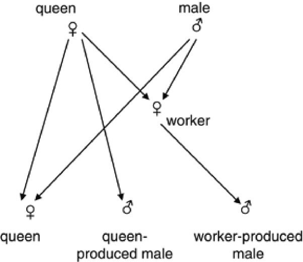
We assume a random mating population of eusocial Hymenoptera with a constant size of Nf queens, Nm (haploid) males and Nw laying workers. The Nm males consist of Nm1 queen-produced and Nm2 worker-produced males, thus the proportion (ϕ) of the worker-produced males being  . Subscripts f, m, w, m1 and m2 are used to specify the cohorts of queens, males, laying workers, queen-produced males and worker-produced males, respectively. The assumed breeding structure is illustrated in Figure 1.
Figure 1.
Assumed breeding structure and gametic pathways.
There are two major definitions of Ne, the variance effective size (Ne(V)), which is defined by the accumulation rate of genetic drift, and the inbreeding effective size (Ne(I)), which is defined by the increasing rate of inbreeding (Crow and Kimura, 1970). Our derivation of expressions for Ne is based on the dentition of Ne(V). Crow and Kimura (1970) has shown that Ne(V) is approximately equal to Ne(I) in a population with a constant mating system and a constant population size over generations. This view will be verified under the examined condition in this study by computer simulation in the later section.
We consider an allele on a neutral locus with the frequency in an arbitrary initial generation as follows:
Queens pf
Laying workers pw
Queen-produced males pm1
Worker-produced males pm2
All males pm=(1−ϕ)pm1+ϕpm2
Owing to genetic drift, the allele frequencies will be changed between generations. With subscripts u and v (=f, m, w, m1 or m2), the change through the gametic pathway from cohorts of u to v is expressed as Δpuv. Furthermore, let Δpf, Δpm1 and Δpm2 be the total change of gene frequency from the parental generation to queens, queen-produced males and worker-produced males in the next generation, respectively. From the mode of haplodiploid inheritance,
 |
 |
The change of gene frequency in worker-produced males (Δpm2) is generated through two steps: step from parents (queens and males) to workers, and step from workers to their sons. Thus, Δpm2 is expressed as
 |
where Δpwm2|pw is the change of gene frequency from workers to their sons for a given pw. The total change of gene frequency in males (Δpm) in the next generation is
Following Hill's (Hill, 1979) idea of the asymptotic contribution of a reproductive cohort in a given generation to remote future, which was introduced to define Ne with overlapping generations, we consider the asymptotic contributions of queens and males in a given generation, which are denoted by cf(∞) and cm(∞), respectively. As shown in Appendix A, they are expressed as
 |
Note that when ϕ=0, cf(∞)=2/3 and cm(∞)=1/3, and these contributions are immediately attained. However, when ϕ>0, the contributions asymptotically converge to cf(∞) and cm(∞). With the asymptotic contributions, the asymptotic contribution of the total change of gene frequency to remote future generations is expressed as
 |
The variance of Δp among an infinite number of conceptual replicated populations is
 |
According to Hill (1979), the effective population size (Ne) is obtained by equating V[Δp] to p(1−p)/2Ne:
 |
where p is the asymptotic average gene frequency in the parental generation, defined by
 |
This definition of average gene frequency was also adopted by Owen and Owen (1989) but without the detailed explanation.
Formulation of the effective population size
From the derivation in Appendix B, we obtain following approximated expressions of V[pf] and V[pm]:
 |
 |
where μuv and  are the mean and variance of the number of progeny in cohort v from a parent in cohort u. Noting μuv=Nv/Nu and Nm1=(1−ϕ)Nm, and substituting (8) into (6) give a general expression of Ne of Hymenopteran population with worker-produced males as
 |
When ϕ=0, equation (9) reduces to
 |
agreeing with the formula obtained by Pollak (1980, 1990), except for omitting the term of covariance among female and male progeny numbers of female parents (queens), which can be neglected if female and male progeny are independently selected.
A compact expression comparable to the formula (1) could be obtained by assuming a Poisson distribution of the progeny number in each gametic pathway, which is a good approximation when the progeny are selected at random. Noting  under a Poisson distribution, we get from (9)
 |
which reduces to the formula (1) when ϕ=0. If the distribution of male progeny number of worker deviates from a Poisson distribution but in other gamaetic pathways the progeny numbers follow a Poisson distribution within each gametic pathway, Ne should be predicted by
 |
where CVwm2(=σwm2/μwm2) is the coefficient of variation of male progeny number per laying worker.
Owen and Owen (1989) derived a formula of Ne for the special case where each laying worker produce exactly one male. In this case, μwm2=1 and  . Assuming again Poisson distributions of the progeny numbers in the other gametic pathways, we obtain from (9)
 |
in accordance with the formula given by Owen and Owen (1989).
Computer simulation
Validity of the obtained equations was checked by computer simulation of genetic drift in the frequency of an allele on a neutral locus. Initial genotypes of Nf queens and Nm males were generated by randomly assigning A1 and A2 alleles with equal frequency (pm=pf=0.5). To obtain the genotype of a young queen, a gamete (gene) picked at random with equal probability from a queen randomly sampled from Nf queens and a gamete from a male randomly sampled from Nm males was united. The sampling of parents (queen and male) and unification of their gametes were repeated until obtaining the genotypes of Nf young queens. In each repetition the sampling of parents was carried out with replacement, allowing both queens and males to have a chance of multiple mating, that is, ‘polyandry–polygyny' model was simulated. The above process to generate young queens is conceptually equivalent to a situation where each parent contributes a large number of candidates for young queens, and young queens are randomly selected from the pooled candidates. The genotypes of Nw laying workers were generated in the same manner. For a queen-produced male, a gene picked at random with equal probability from a randomly sampled (with replacement) queen was assigned. This was replicated to obtain Nm1 queen-produced males. In the basic model of simulation, Nm2 worker-produced males were analogously generated from Nw laying workers. The above reproduction was repeated over a specified number of generations.
In each generation, the frequencies of A1 allele in Nf queens and Nm males were computed. The average gene frequency (pt) in generation t was calculated with equation (7). The simulation was replicated 10 000 times, and the variance of the gene frequency among the replicates  in generation t was computed. Following Spiess (1989), the variance effective population size (Ne(V),t) in generation t was obtained by
 |
where p0 (=0.5) is the initial gene frequency.
As another measure of simulated effective population size, the inbreeding effective population size (Ne(I),t) in generation t was computed from the rate of inbreeding in young queens. The average inbreeding coefficient (Ft) of young queens in generation t was obtained by applying the coancestry method (Falconer and Mackay, 1996) with modification for haplodiploidy and presence of worker reproduction, as described in Appendix C. Following Crow and Kimura (1970), the rate of inbreeding (ΔFt) was computed by
 |
With the average ( ) over 10 000 replicates, the inbreeding effective population size (Ne(I),t) in generation t was obtained by
  .
.
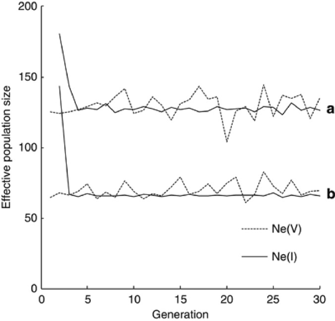
Figure 2 shows the variance and inbreeding effective sizes (Ne(V),t and Ne(I),t) observed over 30 generations in simulated populations with two sets of variables, set A: Nf=Nm=100, ϕ=0.4 and μwm2=2, and set B: Nf=Nm=100, ϕ=0.8 and μwm2=5. Because the first inbred young queens appear in generation 2, Ne(I),t was computed after generation 2. After the initial sharp decline, Ne(I),t essentially attained a steady value. Although Ne(V),t showed a larger fluctuation, the fluctuation seems to be random deviation from an equilibrium value. In all the examined simulations with other sets of variables, similar tendency was observed in the behaviour of Ne(V),t and Ne(I),t. In simulations with a small effective population size as in the variable set B, fixation (or extinction) of an allele occurred in a small proportion (<0.1%) of the replicated populations after generation 25. Inclusion of such replicated populations into the computation of Ne(V),t will result in an overestimation through an underestimation of change in the variance of gene frequency. Viewing these results, the simulated variance and inbreeding effective population sizes were expressed as the harmonic mean over generations 6–20.
Figure 2.
Variance and inbreeding effective population sizes (Ne(V) and Ne(I)) observed during 30 generations of simulated populations with two sets of variables, set (a): Nf=Nm=100, ϕ=0.4 and μwm2=2, and set (b): Nf=Nm=100, ϕ=0.8 and μwm2=5.
In Table 1, the simulated Ne are compared with the prediction from equation (10) for several combination of Nf, Nm and ϕ. In all the cases examined, Ne(V),t and Ne(I),t show an essentially same value, as expected from the relevant theory (Crow and Kimura, 1970). Equation (10) gives a good prediction of both the effective sizes, although it tends to slightly underestimate the simulated effective sizes.
Table 1. Simulated variance and inbreeding effective sizes (N e(V) and N e(I)) and predicted (N e(pre)) effective size of populations with various proportion (ϕ) of worker-produced males, when the progeny number in each gametic pathway follows a Poisson distribution.
| Nf | Nm | μwm2 | ϕ |
Effective size |
||
|---|---|---|---|---|---|---|
| Ne(V) | Ne(I) | Ne(pre) | ||||
| 100 | 100 | 2 | 0.2 | 140.5 | 142.1 | 139.0 |
| 0.4 | 128.1 | 127.2 | 126.1 | |||
| 0.8 | 101.3 | 98.6 | 96.0 | |||
| 5 | 0.2 | 126.3 | 127.3 | 125.6 | ||
| 0.4 | 105.5 | 104.3 | 103.0 | |||
| 0.8 | 68.2 | 65.9 | 65.1 | |||
| 150 | 50 | 2 | 0.2 | 117.3 | 113.2 | 112.6 |
| 0.4 | 95.7 | 92.6 | 92.5 | |||
| 0.8 | 66.1 | 60.3 | 59.3 | |||
| 5 | 0.2 | 103.2 | 99.3 | 96.1 | ||
| 0.4 | 75.7 | 71.8 | 69.6 | |||
| 0.8 | 41.9 | 38.4 | 37.3 | |||
| 50 | 150 | 2 | 0.2 | 100.1 | 97.7 | 97.0 |
| 0.4 | 99.9 | 97.2 | 96.8 | |||
| 0.8 | 94.8 | 92.4 | 91.7 | |||
| 5 | 0.2 | 93.4 | 93.1 | 92.5 | ||
| 0.4 | 91.3 | 87.5 | 86.8 | |||
| 0.8 | 74.4 | 71.1 | 70.3 | |||
Abbreviations: Nf, number of queens; Nm, number of males; μwm2, average number of male progeny per laying worker.
Owen and Owen (1989) simulated two distribution models of the male progeny number per laying worker: the first model is that each laying worker exactly contributes one male, and the second model is that equal numbers of workers produce either 1, 2, 3, 4, or 5 males. Under the first model, they verified that their equation (that is, equation (12) in the present study) leads to a satisfactory prediction. In additional simulations, we checked the validity of our prediction under the second model of Owen and Owen (1989) by comparing simulated Ne with that predicted from equation (11). As shown in Table 2, we again found a good agreement between the simulated and predicted Ne.
Table 2. Simulated variance and inbreeding effective sizes (N e(V) and N e(I)) and predicted (N e(pre)) effective size of populations with various proportion (ϕ) of worker-produced males, when the male progeny number of laying worker follows a uniform distribution with the range from 1 to 5.
| Nf | Nm | Nw | ϕ |
Effective size |
||
|---|---|---|---|---|---|---|
| Ne(V) | Ne(I) | Ne(pre) | ||||
| 100 | 100 | 5 | 0.15 | 144.1 | 140.8 | 139.5 |
| 15 | 0.45 | 120.2 | 116.1 | 116.1 | ||
| 30 | 0.90 | 82.4 | 79.3 | 78.6 | ||
| 50 | 150 | 10 | 0.2 | 99.6 | 95.7 | 96.0 |
| 30 | 0.6 | 95.1 | 92.1 | 91.1 | ||
| 40 | 0.8 | 89.9 | 86.9 | 85.9 | ||
| 150 | 50 | 5 | 0.3 | 97.7 | 96.3 | 96.9 |
| 10 | 0.6 | 71.3 | 67.9 | 67.7 | ||
| 15 | 0.9 | 49.1 | 45.9 | 45.9 | ||
Abbreviations: Nf, number of queens; Nm, number of males; Nw, number of laying workers.
In many eusocial Hymenopteran species, both queens and males mate only once or nearly so (Crozier and Pamilo, 1996; Hughes et al., 2008), which could be approximated by ‘monoandry–monogyny' model. Validity of the obtained equation was also checked under this model. In the simulation, an equal number (N=Nf=Nm) of queens and males were paired to form N fixed couples in each generation. A young queen (or a laying worker) was generated by uniting gametes from a randomly sampled (with replacement) couple. The sampling of couple and unification of their gametes were replicated to obtain Nf young queens (or Nw laying workers). Males were reproduced in the analogous way to the ‘polyandry–polygyny' model. Predicted Ne from equation (10) is compared with the simulated Ne in Table 3. It is verified that under the ‘monoandry–monogyny' model, equation (10) gives a satisfactory prediction of Ne(V),t and Ne(I),t.
Table 3. Simulated variance and inbreeding effective sizes (Ne(V) and Ne(I)) and predicted (Ne(pre)) effective size of populations with various proportion (ϕ) of worker-produced males and monoandry–monogyny mating system.
| Nf | Nm | μwm2 | ϕ |
Effective size |
||
|---|---|---|---|---|---|---|
| Ne(V) | Ne(I) | Ne(pre) | ||||
| 100 | 100 | 2 | 0.2 | 142.5 | 140.2 | 139.0 |
| 0.4 | 130.1 | 127.4 | 126.1 | |||
| 0.8 | 99.3 | 96.6 | 96.0 | |||
| 5 | 0.2 | 130.5 | 127.6 | 125.6 | ||
| 0.4 | 105.7 | 104.4 | 103.0 | |||
| 0.8 | 69.7 | 66.0 | 65.1 | |||
| 300 | 300 | 2 | 0.2 | 423.1 | 418.4 | 417.0 |
| 0.4 | 383.0 | 386.9 | 378.4 | |||
| 0.8 | 289.0 | 288.1 | 288.1 | |||
| 5 | 0.2 | 383.7 | 390.2 | 376.9 | ||
| 0.4 | 314.5 | 311.4 | 309.1 | |||
| 0.8 | 196.6 | 191.9 | 195.2 | |||
Abbreviations: Nf, number of queens; Nm, number of males; μwm2, average number of male progeny per laying worker.
Numerical analysis
To assess the effect of male production by workers on Ne, numerical analysis was carried out. Assuming that the progeny numbers in all the gametic pathways but that from workers to males follow independent Poisson distributions, relative Ne with worker-produced males to that without male production by workers was computed. Using equations (1) and (11), the relative effective size (R) is expressed as
 |
where r=(Nm/Nf) is the breeding sex ratio. In Hymenopteran species, female-baiased breeding sex ratio are very rare, and even when they exists, they are not far from unity. To evaluate the effect of male production by workers on Ne under realistic situations, the low and high ends of r were set at 0.9 and 10, respectively, in the numerical analysis.
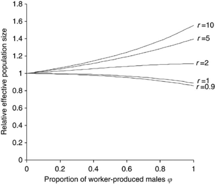
In Figure 3, R is plotted along the proportion of worker-produced males (ϕ) for the cases where each laying worker produces exactly one male (μwm2=1 and CVwm2=0). If the breeding sex ratio is unity or female-biased (r⩽1), the effect of worker-produced males is to slightly reduce Ne. In contrast, when the breeding sex ratio is male-biased (r>1), Ne is increased compared with the value with ϕ=0. The increase in Ne is more prominent for a larger bias in the breeding sex ratio toward male.
Figure 3.
Relative effective size of populations with worker-produced males to that without male production by workers (ϕ=0), when each laying worker exactly produces one male. r, breeding sex ratio (Nm/Nf).
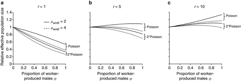
A more realistic situation where some laying workers produce more than one male was examined by considering the combination of two values of μwm2(=2 and 4) and two values of CVwm2:  , where α=1 (variation expected under Poisson distribution) and 2 (variation twice that expected under Poisson distribution). Values of R for the breeding sex ratio r=1, 5 and 10 are plotted along ϕ in Figures 4a, b and c, respectively. As a case with female-biased breeding sex ratio, the breeding sex ratio of r=0.9 was computed, but the result was omitted because it did not largely depart from the result from the unity breeding sex ratio. When the breeding sex ratio is unity (Figure 4a), male production by workers always reduces Ne. Note that the reduction is considerably greater than that in the case of no variation of male progeny number per worker (cf. Figure 3). For example, with the breeding sex ratio r=1 and ϕ=0.5, Ne is reduced by 2.0% when each worker produces a single male (Figure 3), whereas when the male progeny numbers of workers follow a Poisson distribution with μwm2=2, the reduction is 20.6% (Figure 4a). The reduction in Ne is enhanced by an increase in μwm2 and/or CVwm2. If the breeding sex ratio is male-biased (Figures 4b and c), a prominent increase in Ne by worker reproduction is observed only for smaller μwm2 and CVwm2. Unless the breeding sex is extremely biased toward male, the presence of worker-produced males may reduce Ne when μwm2 and/or CVwm2 become larger, as seen in Figure 4b.
Figure 4.
Relative effective size of populations with worker-produced males to that without male production by workers (ϕ=0), when laying workers produce variable numbers of males. r, breeding sex ratio (Nm/Nf); μwm2, average number of male progeny per laying worker; Poisson, male progeny number per laying worker distributes with the coefficient of variation expected under a Poisson distribution; 2 × Poisson, male progeny number per laying worker distributes with the coefficient of variation twice that expected under a Poisson distribution. Results for r=1, 5 and 10 are shown in panels a, b and c, respectively.
Results and Discussion
Crozier and Pamilo (1996) predicted that male production by workers inevitably reduces Ne due to the enhanced genetic drift induced by extra reproduction by workers. The present study, however, showed that a reduction in Ne is not an inevitable consequence of worker reproduction. In a population with male-biased breeding sex ratio, worker reproduction may increase Ne if each laying worker produce a small number of males and the difference of male progeny number among workers is not large.
The honeybee Apis cerana is a good illustrative example for the increased Ne by worker reproduction. Using microsatellite markers, Takahashi (unpublished data) estimated the proportion of worker-produced males (ϕ) in this species to be 34.3% (average over eight colonies). By dissection of workers, he found that 10.2% (average over 8 colonies) of workers per colony have highly developed ovary, but most of them have at most one mature egg in their ovaries. This observation suggests that most of the worker-produced males are from different workers, that is, μwm2≈1 and  . Koyama et al. (2009) estimated that a queen of this species mates nine drones on average. As each drone mates only once, the breeding sex ratio is estimated to be r=9. Substituting these estimated values into (13) gives a relative effective size of 1.12. Thus, the male production by workers in A. cerana increases Ne by 12%, compared with the population without worker-produced males.
In populations with unity or female-biased breeding sex ratio, worker reproduction always reduces Ne. Even in population with male-biased breeding sex ratio, Ne may be reduced by worker reproduction when laying workers contribute highly variable numbers of males. The reduction in Ne could be illustrated with a population of the wasp Polistes chinensis. From the data given by Tsuchida et al. (2003); Wenseleers and Ratnieks (2006) estimated the proportion of worker-produced males (ϕ) to be 51.1%. Assuming unity breeding sex ratio (r=1) and a Poisson distribution of the progeny number in each gametic pathway, the reduction in Ne predicted from (13) is 21.2% for μwm2=2. The reduction increases to 34.0% when μwm2=4.
The bumblebee Bombus sylvarum could be another example to illustrate the importance for incorporating the effect of worker reproduction into the estimation of Ne. Assuming monogamous mating and Nf=Nm=32 (which is the estimated number of nests), and using formula (1), Ellis et al. (2006) estimated Ne of an isolated population (Castlemartin) of B. sylvarum in UK to be 48, whereas a three times less estimate (16.4) of Ne was obtained for this population from the changes in allele frequency at microsatellite loci. Although the proportion (ϕ) of worker-produced males in this species is not known, significant levels (20–80%) of worker-produced males have been reported in many Bombus species (Crozier and Pamilo, 1996; Brown et al., 2003). Assuming Nf=Nm=32 and μwm2=4, equation (10) gives estimates of Ne=35.1 for ϕ=0.4, and Ne=23.3 for ϕ=0.8. In a recent work, Huth-Schwarz et al. (2011) reported that the proportion of worker-produced males in the neotropical bumblebee B. wilmattae is 96.7%. When this proportion is assumed, the estimate of Ne is further reduced to 19.1. These estimates suggest that a large part of the difference between the two estimates (48 vs 16.4) of Ne reported by Ellis et al. (2006) might be ascribed to the effect of worker reproduction.
Hymenopteran species usually exhibit lower levels of genetic variation, when compared with diploid species (reviewed by Packer and Owen (2001)). Crozier and Pamilo (1996) predicted that although male production by workers may lead to lower levels of genetic variation by its effect on Ne, it is unlikely that the effect is larger. However, as shown in the present study, worker reproduction could be a critical source to limit genetic variation through a reduction in Ne.
Ne has a special importance in Hymenopteran species with complementary sex determination (CSD), because it determines allelic diversity at the CSD locus (Yokoyama and Nei, 1979; Page and Marks, 1982; Zayed, 2009). Populations with a smaller Ne maintain less alleles at the CSD locus, and consequently produce higher frequencies of sterile or effectively lethal diploid males. As suggested by Zayed and Packer (2005), this phenomenon can lead to ‘an extinction vortex'. Furthermore, Zayed (2004) showed that CSD itself may drastically reduce Ne by the loss of breeding males through diploid male production. The present study suggests that worker reproduction could be an additional factor to critically reduce Ne and should be incorporated into population and conservation genetic models of Hymenopteran populations with CSD.
Data archiving
Data have been deposited at Dryad: doi: 10.5061/dryad.7p838r83.
Acknowledgments
This work was in part financially supported by the Japan Beekeeping Association.
Appendix A
Derivation of equation (5)
Let πuv be the contribution of parents of cohort u (=m or f) to progeny of cohort v (=m or f). Clearly,
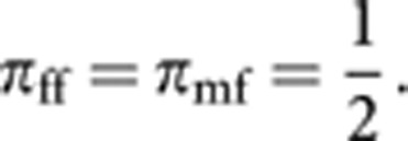 |
The contribution πfm consists of two components: the direct contribution of queens, and the contribution through laying workers, which are expected to be 1−ϕ and ϕ/2, respectively. Thus,
 |
As males contribute to male progeny only through laying workers,
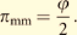 |
We define a transition matrix P and vectors cf(0) and cm(0) as
 |
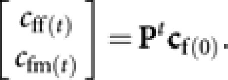
The contributions of queens in a given generation (generation 0) to queens and males in generation t, cff(t) and cfm(t), respectively, are obtained as
 |
Similarly, the contribution of males in generation 0 to queens and males in generation t, cmf(t) and cmm(t), respectively, are
 |
Since P is a stochastic matrix describing a two-state Markov chains, from the relevant theory of stochastic process (for example, Bhat, 1984), Pt is expressed as
 |
where
 |
Since x→0 and y→0 for t→∞,
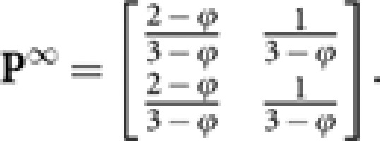 |
Then,
 |
giving
 |
Analogously, we get from P∞cm(0)
 |
Appendix B
Derivation of equation (8)
From (2), the variance of Δpf is
 |
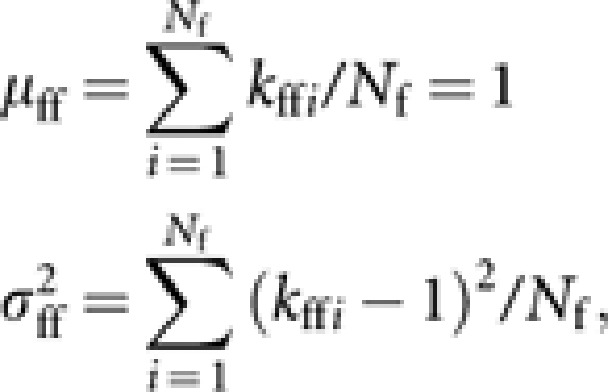
Take V[Δpff] as an example of the derivation. Following the approach described by Crow and Denniston (1988) and Caballero (1994), let kffi be the number of young queens contributed by queen i, with the mean (μff) and variance  ,
,
 |
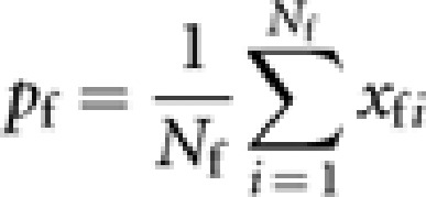
and xfi (=0, 1/2 or 1) be the gene frequency in queen i. The gene frequency in queens is
 |
and the gene frequency in Nf genes of young queens contributed by queens is
 |
where δij is the difference in gene frequency between jth sampled gene and its parental value xfi (δij is zero if queen i is a homozygote, or ±1/2 if a heterozyote). Then,
 |
Following the retrospective approach in defining the effective population size from the observed numbers of progeny per parent (Crow and Kimura, 1970; Caballero, 1994), we regard kffi as a fixed variable. This gives
 |
According to Caballero (1994), approximated expressions of V[xfi] and V[δij] are  and
and  . With these expressions, we obtain
 |
Applying a similar approach and noting that males are haploids, we obtain an expression of V[Δpmf] as
 |
Approximating pf and pm by the average gene frequency p, that is,
and substituting (A2) and (A3) into (A4) give equation (8a) in the text. Approximation (A4) is reasonable, because the difference of gene frequency between queens and males in a generation asymptotically disappears, as predicted from the deterministic analysis by Owen (1980).
Next, consider the variance of Δpm. From (4), the variance is expressed as
The derivation applied to obtain (A2) gives
 |
From (3), V[Δpm2] is written as
 |
where E[ ] is the expectation taken for pw. With the analogous derivation applied to (A2) and (A3), we have
 |
and
 |
Furthermore, applying an approximation E[pw(1−pw)]=p(1−p) and an analogous derivation to (A2), we have an expression of the final term in (A7) as
 |
Substituting (A8–10) into (A7) and applying the approximation (A4) give
 |
Finally, substituting (A6) and (A11) into (A5), and again applying the approximation (A4) lead to equation (8b) in the text.
Appendix C
Modified coancestry method applied to computation of inbreeding coefficient in simulated populations
For the computation of inbreeding coefficients of young queens, the coancestry method described by Falconer and Mackay (1996) was applied with modifications for haplodiploidy and presence of worker reproduction. We first define a coancestry matrix among young queens and males in generation t as
 |
where θff,t is a matrix (with order Nf × Nf) containing coancestries among Nf young queens, θmm,t is a matrix (with order Nm × Nm) containing coancestries among Nm males, θfm,t is a matrix (with order Nf × Nm) containing coancestries between Nf young queens and Nm males, and θ′fm,t is the transposed matrix of θfm,t. For the initial generation (t=0), θfm,0 is a null matrix, and θff,0 and θmm,0 are diagonal matrices:
When parentages of young queens and males are known, all the elements of θt can be expressed with elements of θt−1.
Take elements of θmm,t as an example. As males are haploid, self-coancestry (θm(i)m(i),t) of a male (m(i); i=1, 2, …, Nm), which is a diagonal element of θmm,t, is apparently
 |
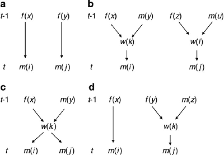
To obtain expressions for coancestry among different males (m(i) and m(j); i, j=1, 2, …, Nm and i≠j), following four cases should be considered.
Case a: Two queen-produced males (Figure C1a).
Figure C1.
Four cases of relationship among two males (m(i) and m(j)) to be considered in construction of coancestry matrix in generation t. (a) Two queen-produced males; (b) Two worker-produced males from different workers; (c) Two worker-produced males from same worker; (d) Queen-produced and worker-produced males. f and m, queen and male in generation t−1; w, laying worker.
By definition, coancestry among m(i) and m(j) is equal to coancestry among their mothers (f(x) and f(y)):
 |
Case b: Two worker-produced males from different workers (Figure C1b)
Coancestry among m(i) and m(j) is equal to coancestry among their mothers (workers w(k) and w(l)). Then, with the standard rule of coancestry (Falconer and Mackay, 1996),
 |
Case c: Two worker-produced males from same worker (Figure C1c)
Coancestry among m(i) and m(j) is equal to self-coancestry of the common mother (worker w(k)). Then
 |
Case d: Queen-produced and worker-produced males (Figure C1d)
Coancestry among m(i) and m(j) is equal to coancestry among their mothers (queen f(x) and worker w(k)). Then
 |
With an analogous way, the remaining elements of θt can be related to elements of θt−1. The inbreeding coefficient (Ff(i),t) of a young queen in generation t is obtained by coancestry among their mother and father (f(x) and m(y)) as Ff(i),t=θf(x)m(y),t−1, which is an element of θfm,t−1.
The authors declare no conflict of interest.
References
- Bhat UN. Elements of Applied StochasticProcess. John Wiley & Sons: New York; 1984. [Google Scholar]
- Brown MJF, Schmid-Hempel R, Schmid-Hempel P. Queen-controlled sex ratios and worker reproduction in the bumble bee Bombus hypnorum, as revealed by microsatellites. Mol Ecol. 2003;12:1599–1605. doi: 10.1046/j.1365-294x.2003.01840.x. [DOI] [PubMed] [Google Scholar]
- Caballero A. Developments in the prediction of effective population size. Heredity. 1994;73:657–679. doi: 10.1038/hdy.1994.174. [DOI] [PubMed] [Google Scholar]
- Contel EPB, Kerr WE. Origin of males in Melipona subnitida estimated from data of an isozymic polymorphic system. Genetica. 1976;46:271–277. [Google Scholar]
- Crow JF, Denniston C. Inbreeding and variance effective population numbers. Evolution. 1988;42:482–495. doi: 10.1111/j.1558-5646.1988.tb04154.x. [DOI] [PubMed] [Google Scholar]
- Crow JF, Kimura M. An Introduction to Population Genetics Theory. Harper & Row: New York; 1970. [Google Scholar]
- Crozier RH, Pamilo P. Evolution of Social Insect Colonies. Sex Allocation and Kin Selection. Oxford University Press: Oxford; 1996. [Google Scholar]
- Ellis JS, Knight ME, Darvill B, Goulson D. Extremely low effective population size, genetic structuring and reduced genetic diversity in a threatened bumblebee species, Bombus sylvarum (Hymenoptera: Apidae) Mol Ecol. 2006;15:4375–4386. doi: 10.1111/j.1365-294X.2006.03121.x. [DOI] [PubMed] [Google Scholar]
- Falconer DS, Mackay TFC.1996Introduction to Quantitative Genetics4th edn.Longman: Essex [Google Scholar]
- Frankham R, Ballow JD, Briscoe DA. Introduction to Conservation Biology. Cambridge University Press: Cambridge; 2002. [Google Scholar]
- Hamilton WD. The genetical evolution of social behavior. I, II. J Theor Biol. 1964;7:17–52. doi: 10.1016/0022-5193(64)90039-6. [DOI] [PubMed] [Google Scholar]
- Hill WG. A note on effective population size with overlapping generations. Genetics. 1979;92:317–322. doi: 10.1093/genetics/92.1.317. [DOI] [PMC free article] [PubMed] [Google Scholar]
- Hughes WHO, Oldroyd BP, Beekman M, Ratnieks FLW. Ancestral monogamy shows kin selection is key to the evolution of eusociality. Science. 2008;320:1213–1216. doi: 10.1126/science.1156108. [DOI] [PubMed] [Google Scholar]
- Huth-Schwarz A, León A, Vandame R, Moritz RFA, Kraus FB.2011Workers dominate male production in the neotropical bumblebee Bombus wilmattae (Hymenoptera: Apidae) Front Zool 813[online] URL. . http://www.frontiersinzoology.com/content/8/1/13 . [DOI] [PMC free article] [PubMed] [Google Scholar]
- Koyama S, Takagi T, Martin SJ, Yoshida T, Takahashi J. Absence of reproductive conflict during queen rearing in Apis cerana. Insect Soc. 2009;56:171–175. [Google Scholar]
- Owen RE. Population genetics of social Hymenoptera with worker-produced males. Heredity. 1980;45:31–46. [Google Scholar]
- Owen RE, Owen ARG. Effective population size in social Hymenoptera with worker-produced males. Heredity. 1989;63:59–65. doi: 10.1038/hdy.2012.11. [DOI] [PMC free article] [PubMed] [Google Scholar]
- Packer L, Owen R.2001Population genetic aspects of pollinator decline Conserv Ecol 54[online] URL. . http://www.consecol.org/vol5/iss1/art4 . [Google Scholar]
- Page RE, Marks RW. The population genetics of sex determination in honey bees: random mating in closed populations. Heredity. 1982;48:263–270. [Google Scholar]
- Pollak E. Effective population numbers and mean times to extinction in dioecious populations with over lapping generations. Math Biosci. 1980;52:1–25. [Google Scholar]
- Pollak E. The effective population size of an age-structured population with a sex-linked locus. Math Biosci. 1990;101:121–130. doi: 10.1016/0025-5564(90)90105-8. [DOI] [PubMed] [Google Scholar]
- Queller DC, Peters JM, Solis CR, Strassmann JE. Control of reproduction in social insect colonies: individual and collective relatedness preferences in the paper wasp, Polistes annularis. Behav Ecol Sociobiol. 1997;40:3–16. [Google Scholar]
- Spiess EB. Genes in Populations. John Wiley & Sons: New York; 1989. [Google Scholar]
- Trivers RL, Hare H. Haplodiploidy and the evolution of the social insects. Science. 1976;191:249–263. doi: 10.1126/science.1108197. [DOI] [PubMed] [Google Scholar]
- Tsuchida K, Saigo T, Nagata N, Tsujita S, Takeuchi K, Miyano S. Queen-workwe conflicts over male production and sex allocation in a primitively eusocial wasp. Evolution. 2003;57:2265–2373. doi: 10.1111/j.0014-3820.2003.tb00248.x. [DOI] [PubMed] [Google Scholar]
- Wenseleers T, Ratnieks FLW. Enforced altruism in insect societies. Nature. 2006;442:50. doi: 10.1038/444050a. [DOI] [PubMed] [Google Scholar]
- Wenseleers T, Helanterä H, Hart A, Ratnieks FLW. Worker reproduction and policing in insect societies: an ESS analysis. J Evol Biol. 2004;17:1035–1047. doi: 10.1111/j.1420-9101.2004.00751.x. [DOI] [PubMed] [Google Scholar]
- Wright S. Inbreeding and homozygosis. Proc Natl Acad Sci USA. 1933;19:411–420. doi: 10.1073/pnas.19.4.411. [DOI] [PMC free article] [PubMed] [Google Scholar]
- Yokoyama S, Nei M. Population dynamics of sex-determining alleles in honey bees and self-incompatibility alleles in plants. Genetics. 1979;91:609–626. doi: 10.1093/genetics/91.3.609. [DOI] [PMC free article] [PubMed] [Google Scholar]
- Zayed A. Effective population size in Hymenoptera with complementary sex determination. Heredity. 2004;93:627–630. doi: 10.1038/sj.hdy.6800588. [DOI] [PubMed] [Google Scholar]
- Zayed A. Bee genetics and conservation. Apidologie. 2009;40:237–262. [Google Scholar]
- Zayed A, Packer L. Complementary sex determination substantially increases extinction proneness of haplodiploid populations. Proc Natl Acad Sci USA. 2005;102:10742–10746. doi: 10.1073/pnas.0502271102. [DOI] [PMC free article] [PubMed] [Google Scholar]


