Actual and Counterfactual Smoking Prevalence Rates in the US population via Micro-simulation

Abstract

The Smoking History Generator (SHG) developed by the National Cancer Institute simulates individual life/smoking histories that serve as inputs for the Cancer Intervention and Surveillance Modeling Network (CISNET) lung cancer models. In this chapter, we review the SHG inputs, describe its outputs, and outline the methodology behind it. As example, we use the SHG to simulate individual life histories for individuals born between 1890 and 1984 for each of the CISNET smoking scenarios and use those simulated histories to compute the corresponding smoking prevalence over the period 1975–2000.

1 INTRODUCTION

Micro-simulation models produce individual observations. Rather than sample the entire population, each observation is generated using a pseudo random number generator using distributions based on characteristics of a specific population. For the Cancer Intervention and Surveillance Modeling Network (CISNET) lung cancer models, the relevant population was all males and females ages 30–84 years in the US population over the period 1975–2000. It was necessary to distinguish this population by smoking status, specifically in terms of never, current and former smokers. The former smokers were further categorized by the number of years since quitting smoking. Smokers and ex-smokers were also characterized by their smoking duration and smoking intensity. To generate simulated natural histories, smoking patterns had to be developed over the lifetime of the simulated individual. To accomplish these aims, the smoking history generator (SHG) was developed to provide a common source for smoking pattern data from which to assess the impact of tobacco control efforts.

The SHG is a shared precursor model that produces cohort-specific smoking histories and related other-cause death rates (i.e., non-lung cancer deaths) as inputs for larger dose/response survival generation models. This shared input source provides a control for smoking history and other-cause mortality aspects of the simulations performed that is common across all CISNET models. The core SHG software was parameterized using three distinct smoking scenarios to produce the requisite input data for the models. The first, called the actual tobacco control (ATC) scenario, is a quantitative description of actual smoking behaviors of males and females born in the US between 1890 and 1984. The second, called no tobacco control (NTC), is a quantitative description of predicted smoking behaviors of US population under the assumption that tobacco control efforts starting mid-century had never been implemented (see Chapter 4 of this monograph⁽¹⁾). The third, called complete tobacco control (CTC), is a quantitative description of predicted smoking behaviors of US population under the assumption that tobacco control activities yielded perfect compliance, with all cigarette smoking coming to an end in the mid-sixties (see Chapter 4 of this monograph⁽¹⁾). The ATC scenario used inputs derived directly from observed data in the National Health Interview Surveys (NHIS) and the Substance Abuse and Mental Health Services Administration (SAMHSA) National Survey on Drug Use and Health (see Chapter 2 of this monograph⁽²⁾). The NTC scenario used inputs derived by extrapolating from trends in the observed histories before 1954, i.e., before any tobacco control in the decade leading up to the publication of the Surgeon General’s Report in 1964. The CTC scenario was simulated by setting cessation rates to one (i.e., transferring all current smokers to former smokers) and allowing no further initiation starting in 1965 while using the observed values in earlier years.

The outputs of the SHG are used by each individual lung cancer model in CISNET to stratify the population by smoking histories. Some models can be characterized as individual cohort models, meaning that they utilize as inputs individual smoking histories from birth as part of biologically-based models of carcinogenesis to determine when lung cancer death occurs.^(3–6) Other models can be characterized as group cross-sectional models, with inputs comprised of a cross-sectional picture defined by calendar-year, gender, and age-specific proportions of the population stratified by smoking status. While the SHG was originally developed for the individual cohort models, estimates of grouped data were needed for the group cross-sectional models to have a common input base across all models.

In this chapter, we review the inputs of the SHG, describe its outputs, and briefly summarize the methodology behind it. Using the SHG, we simulated 15,000 individual life histories per birth year from 1890 until 1984 for both males and females in the US for each of the three CISNET smoking scenarios, and used those individual life histories to compute and compare the prevalence of smoking under the three smoking scenarios.

2 METHODS

2.1 The smoking history generator

2.1.1 SHG Inputs

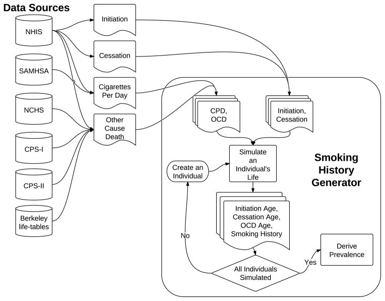
The SHG utilizes input data from several sources, including the NHIS data from 1965 to 2001 and the SAMHSA data (see Chapter 2 of this monograph⁽²⁾), the Berkeley mortality database cohort life-tables, the National Center for Health Statistics (NCHS), the Cancer Prevention Study I and II (CPS-I and CPS-II), and the Nutrition follow-up studies sponsored by the American Cancer Society (see Chapter 3 of this monograph⁽⁷⁾). The NHIS and the SAMHSA datasets provide estimates for prevalence of never, former (by years quit) and current smokers by age and year, and data on smoking intensity (in terms of the average number of cigarettes smoked per day (CPD)). These data were used to create implicit initiation and cessation rates, while adjusting for the differential mortality of ever smokers in comparison with that of never smokers to correct for biases in the retrospective reconstruction of initiation rates (see Chapter 2 of this monograph⁽²⁾ for more details). Using the average initiation rate, the SHG is able to determine the probability that a never smoker becomes a smoker per year. For those individuals who are smokers, the cessation rates are used to determine the annual probability that a smoker becomes an ex-smoker. The Berkeley life-tables, combined with smoking prevalence estimates from NHIS and the relative risks of death for smokers and former smokers in comparison to never smokers from CPS-I and CPS-II, are used to produce the probability of death from causes other than lung cancer based on age, gender, birth cohort, and smoking status. Fig. 1 shows a flow diagram of the SHG, and Table I summarizes the input sources for the SHG for the three CISNET smoking scenarios.

Fig. 1.

Flow diagram of the Smoking History Generator

Table I.

Inputs for the SHG

Input	ATC	NTC	CTC
Initiation rates	NHIS (see Chapter 2(2))	Derived (see Chapter 4(1))	Derived (see Chapter 4(1)) (no new smokers after 1965)
Cessation rates	NHIS (see Chapter 2(2))	Derived (see Chapter 4(1))	Derived (see Chapter 4(1)) (all smokers quit in 1965)
CPD1	NHIS, SAMHSA (see Chapter 2(2))
OCD2	Berkeley life-tables, NCHS, NHIS, CPS-I, CPS-II, Nutrition Follow-up studies (see Chapter 3(7))
Birth year (1890 – 1984)	User defined
Gender (Male/Female)	User defined
Race (All race)	User defined

¹Cigarettes smoked per day.

²Other cause death.

ATC: actual tobacco control, NTC: no tobacco control, CTC: complete tobacco control.

The SHG accepts parameters supportive of the three smoking scenarios described above (see Table I). The ATC scenario uses initiation, cessation and smoking intensity (CPD) rates directly derived from the NHIS and SAMHSA datasets (see Chapter 2 of this monograph⁽²⁾). The NTC scenario uses initiation and cessation rates derived by fitting an age-period-cohort model to the ATC rates up to 1954, i.e., before the appearance of any tobacco control measures, and by projecting those into the future maintaining them consistent with the patterns observed in 1954 (see Chapter 4 of this monograph⁽¹⁾). The CTC scenario uses initiation and cessation rates identical to those of the ATC scenario up to 1965, and then sets the cessation rates equal to one and the initiation rates equal to zero, i.e., all smokers are forced to quit in 1965, and no new smokers are allowed to appear thereafter. All scenarios use smoking dependent other cause death (OCD) rates derived from several sources as mentioned above (see Chapter 3 of this monograph⁽⁷⁾).

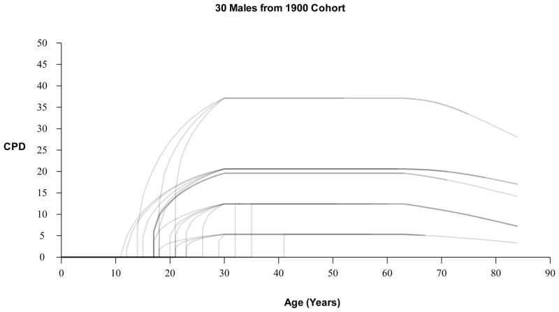
Dose is determined by the individual’s smoking intensity quintile, which is assigned as a function of initiation age. More specifically, if an individual initiates smoking, the SHG classifies the individual into one of five smoking intensity groups, based on the probabilities of being a light to heavy smoker as a function of initiation age. Smoking intensity quintiles determine the smoker’s mean CPD starting from age 30 and are based on race, gender and birth cohort. For years between initiation age and age 30, the smoker’s CPD is modeled as monotonically increasing from initiation. The uptake formula depends on age, duration, year, and is fit to exactly match the age 30 mean CPD designated by the individual’s smoking intensity quintile. See Appendix A.1 for details on the uptake formula. Fig. 2 presents examples of smoking dose (CPD) profiles for 30 males from the 1900 birth cohort.

Fig. 2.

Examples of smoking dose (CPD) profiles for 30 males from the 1900 birth cohort.

2.1.2 SHG Outputs

The inputs of the SHG are used to simulate life histories (up to age 84) for individuals born in the US between 1890 and 1984. These life histories include a birth year, and age at death from causes other than lung cancer, conditioned on smoking histories. For each simulated individual, the generated life histories include whether the individual was a smoker or not and, if a smoker, the age at smoking initiation, the smoking intensity (CPD) by age, and the age of smoking cessation (See Fig. 1). Smoking relapse, the probability that a former smoker starts smoking again, is not modeled. More details about the computational algorithm behind the SHG are given in Appendix A.

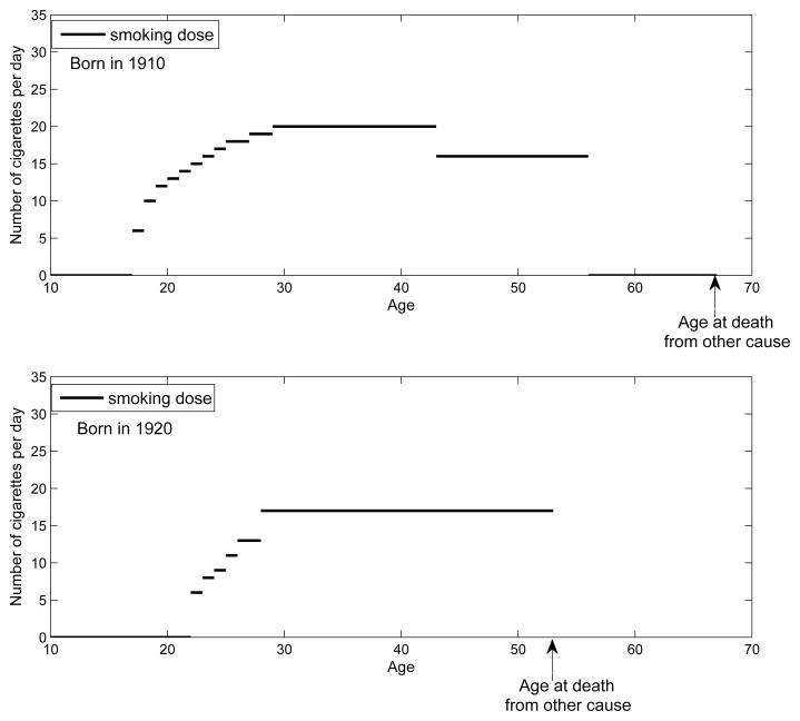
Table II summarizes the output of the SHG, and Fig. 3 shows two examples of smoking histories simulated by the SHG; a) an individual born in 1910 who begins smoking at age 17, quits at age 56 and dies at age 67 due to causes other than lung cancer, and b) an individual born in 1920 who begins smoking at age 22 and dies at age 53 due to causes other than lung cancer.

Table II.

Output variables of the SHG

Initiation Age	Age at smoking initiation
Cessation Age	Age at smoking cessation
OCD1 Age	Age at death from cause other than lung cancer
Smoking History	Smoking intensity quintile (5 quintiles ranging from light to heavy smoking), Yearly smoking dose (CPD2)

¹Other cause death.

²Cigarettes smoked per day.

Fig. 3.

Examples of the SHG-generated events.

The SHG can produce smoking histories consistent with each of the three CISNET smoking scenarios described above (see Table I). In the case of the ATC scenario, the smoking patterns in the simulated individuals, resulting from the combined event of lung cancer death superimposed over the SHG-generated life histories, agree with the observed ones in the US population (see Validation and Consistency Checks below).

2.2 Generation of prevalence tables using simulated individual life histories for the US population

The main purpose of the CISNET Lung Smoking Base Case is to evaluate the effects of smoking interventions on lung cancer mortality rates in the US. The SHG was used to simulate detailed smoking information for individuals born between 1890 and 1984 under each of the three smoking scenarios. Among the CISNET models, the individual cohort models use the individual information directly, while the group cross-sectional models require average statistics by age and birth year. To provide inputs for the group cross-sectional models, we computed tables that summarize the smoking experience of the population by using the SHG-generated individual life histories for each of the three smoking scenarios.

Specifically, we generated smoking prevalence tables for US males and females by smoking status (never, current, former smokers), average smoking intensity for current and former smokers (CPD), average smoking initiation age for current and former smokers, average smoking duration for current smokers, and average years since quitting smoking for former smokers. These tables were provided as inputs for the group cross-sectional models.

To generate the prevalence tables, we first simulated 15,000 individual life histories per birth year from 1890 until 1984 for both males and females using the SHG. At each age, simulated individuals were distributed into three categories according to their smoking status: never, current, and former smokers. The former smokers were further classified into five sub-categories depending on the number of years since quitting: 1–2 years, 3–5 years, 6–10 years, 11–15 years, more than 16 years. Because the SHG does not account for death from lung cancer in its simulations, it produces an excess of ever smokers, especially among the oldest ages, in comparison with the US population. To remedy this inconsistency, we adjusted the SHG-generated life histories by incorporating lung cancer mortality using one of the CISNET models. The details of this adjustment are described in the Appendix B. With the simulated life histories, we generated smoking prevalence tables by birth cohort, calendar year, smoking status, and gender. Similarly, we also generated tables containing the mean number of CPD, the mean duration of smoking, and the mean age of smoking initiation for current and former smokers.

2.2.1 Validation and Consistency Checks

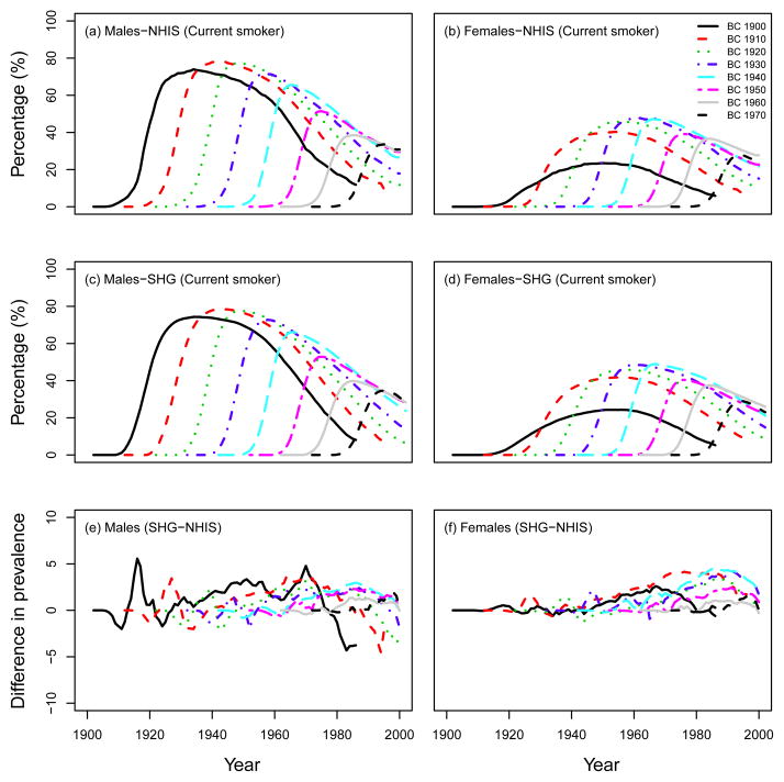
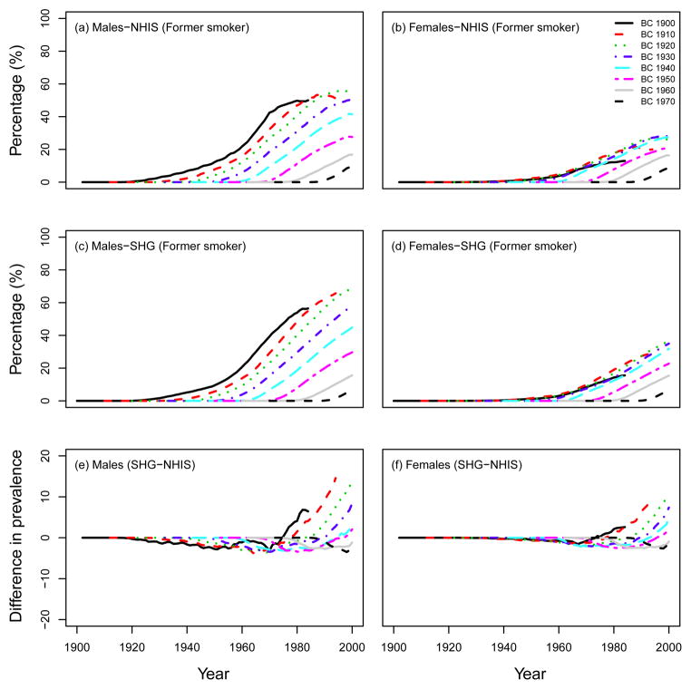
To validate the performance of the SHG, we checked the consistency in smoking patterns (e.g., smoking prevalence, smoking intensity, smoking duration) between the observed data from the NHIS and outputs of the SHG (ATC scenario). Note that, as mentioned above, we had to adjust the SHG-generated life histories by incorporating lung cancer mortality using one of the CISNET models (See Appendix B). For example, Fig. 4 shows the percentage of current smokers in US males and females for several birth cohorts (top row: observed data from the NHIS, middle row: computed prevalence using 15,000 simulated individual life histories for each birth cohort from the SHG). Fig. 4 also shows the difference (percentage) between the observed prevalence of current smokers and the predictions from the SHG (bottom row). As seen in Fig. 4 the SHG produces smoking histories that match closely the prevalence levels observed in the US population, i.e., the predicted prevalence from the SHG-generated data is within 5 percentage points of the NHIS observed data. A similar figure comparing the SHG predictions with the prevalence of former smokers in NHIS is presented in Fig. 5. In this case, the former smoker prevalence from the SHG is also fairly consistent with that observed in the NHIS, with the exception perhaps of former smokers of ages 80 or older. This discrepancy for older former smokers may be explained in part by the assumptions on cessation and lack of relapse in the SHG as well as by the potential misclassification of long-term former smokers (long-term quitter) as never smokers in the NHIS data^(8–9) (see discussion). Notice that the larger discrepancies in these figures are mostly for the largest prevalence values, which in relative terms would translate into small differences.

Fig. 4.

Percentage of current smokers in US males and females. Top row: observed data from the NHIS survey, middle row: computed prevalence using the SHG-generated data, adjusted for lung cancer deaths (ATC scenario). Bottom row: Difference between SHG-generated prevalence (SHG) and observed prevalence (NHIS), calculated by SHG-NHIS. BC=birth cohort.

Fig. 5.

Percentage of former smokers in US males and females. Top row: observed data from the NHIS survey, middle row: computed prevalence using the SHG-generated data, adjusted for lung cancer deaths (ATC scenario). Bottom row: Difference between SHG-generated prevalence (SHG) and observed prevalence (NHIS), calculated by SHG-NHIS. BC=birth cohort.

3 RESULTS

3.1 Comparison of smoking prevalence between the three CISNET smoking scenarios

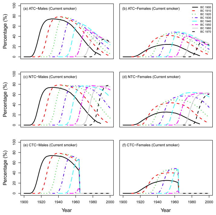
Fig. 6 shows the prevalence of current smokers for several birth cohorts under the three CISNET smoking scenarios (ATC, NTC, CTC) for US males and females.

Fig. 6.

Prevalence of current smokers in US males and females in several birth cohorts, which were computed using the SHG-generated data, adjusted for lung cancer deaths. Three CISNET smoking scenarios; ATC: actual tobacco control, NTC: no tobacco control, CTC: complete tobacco control.

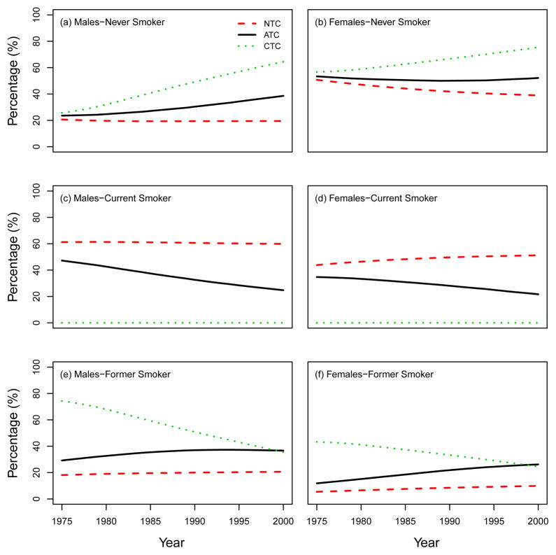
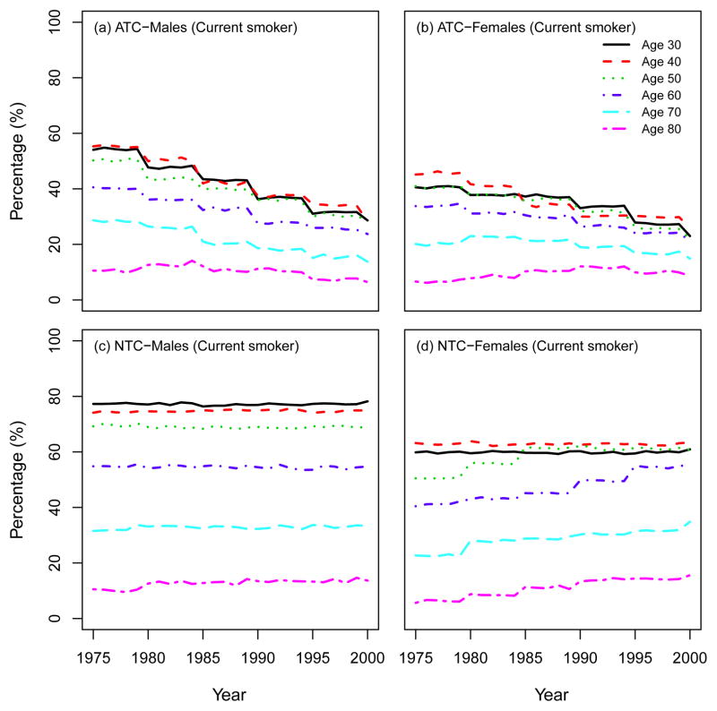
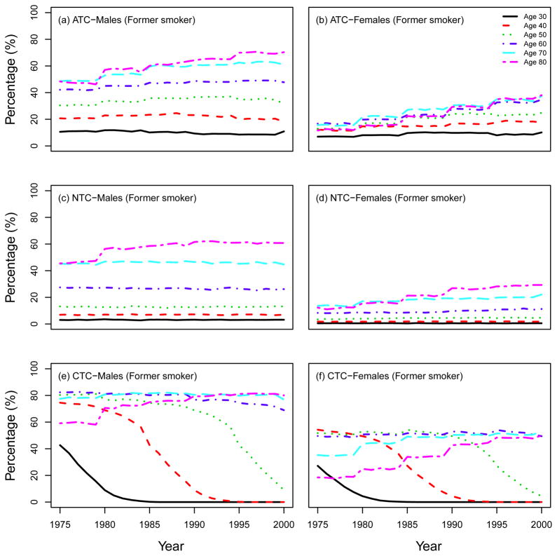
We also present other summary statistics of smoking prevalence and smoking patterns under the three CISNET smoking scenarios. From this point forward we will follow the same structure as the CISNET Lung Smoking Base Case, whereby all results are confined to ages 30–84 years over the period 1975–2000. Fig. 7 shows the percentage of never, current and former smokers in the three CISNET smoking scenarios by calendar year for both males and females. As mentioned above, the ATC scenario represents the smoking levels actually experienced by the US population, so the percentages under this scenario are consistent with those observed in the US. In particular, the percentage of current smokers over the period covered decreased from about 47% in 1975 to 25% in 2000 among males and from about 35% to 22% among females. The percentage of never smokers increased from about 24% in 1975 to 39% in 2000 among males, while the prevalence of never smokers remained more or less constant among females (≈ 50%). In contrast, in the NTC scenario there were no explicit changes in smoking trends for both males and females. In the CTC scenario, the more extreme smoking intervention, more rapid changes in smoking levels are observed in comparison with the ATC. Fig. 8 and Fig. 9 show the percentage of current and former smokers by age and calendar year for males and females. Notice that there are no current smokers in the CTC scenario starting in 1965. A similar figure for never smokers is shown in a separate chapter (see Chapter 6 of this monograph⁽¹⁰⁾). These figures show the dramatic difference in the levels of smoking experienced between the three CISNET smoking scenarios.

Fig. 7.

Percentage of never, current, and former smokers under the three CISNET smoking scenarios; NTC: no tobacco control, ATC: actual tobacco control, CTC: complete tobacco control. All the results are confined to ages 30–84 by following the same structure as the CISNET Lung Smoking Base Case.

Fig. 8.

Prevalence of current smokers according to single ages (30; 40; 50; 60; 70; 80). ATC: actual tobacco control, NTC: no tobacco control.

Fig. 9.

Prevalence of former smokers according to single ages (30; 40; 50; 60; 70; 80). ATC: actual tobacco control, NTC: no tobacco control, CTC: complete tobacco control.

3.2 Comparison of smoking intensity between the three CISNET smoking scenarios

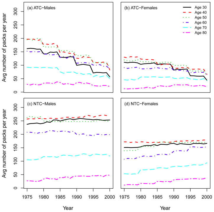
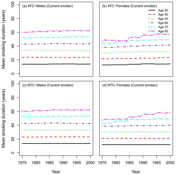
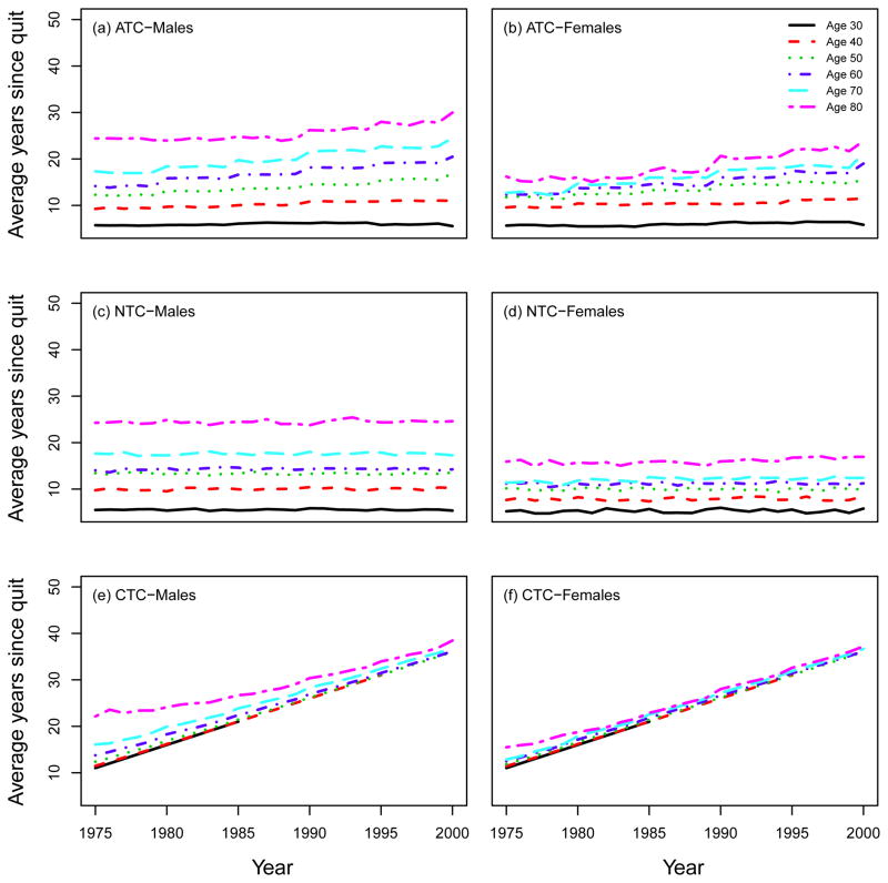
Using the SHG, the distribution of the smoking intensities (CPD) can be computed by age and calendar year. Moreover, the SHG can be used to compute other standard epidemiological measures of smoking exposure, like the average number of packs of cigarettes smoked per year (1975 – 2000). Fig. 10 shows that there is a decrease in smoking intensity by calendar year in the ATC scenario for both males and females, especially among young people, while no trend appears in the NTC. Fig. 11 shows the mean smoking duration of current smokers according to single ages by calendar year, indicating no difference between ATC and NTC for both males and females. This occurs because, although in the NTC scenario fewer people quit smoking, those who remain as current smokers do so at levels comparable to those in the ATC scenario. Fig. 12 shows the average years since quitting smoking of former smokers under each smoking scenario for males and females.

Fig. 10.

Average number of packs of cigarettes smoked per year according to single ages (30; 40; 50; 60; 70; 80). ATC: actual tobacco control, NTC: no tobacco control.

Fig. 11.

Mean smoking duration of current smokers according to single ages (30; 40; 50; 60; 70; 80). ATC: actual tobacco control, NTC: no tobacco control.

Fig. 12.

Average years since quitting smoking of former smokers according to single ages (30; 40; 50; 60; 70; 80). ATC: actual tobacco control, NTC: no tobacco control, CTC: complete tobacco control.

3.3 Sensitivity analysis for the year to quit smoking in the CTC scenario

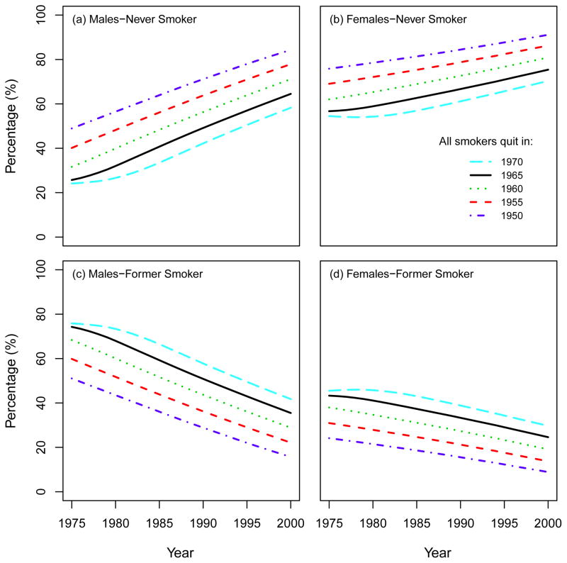
Under the CTC smoking scenario, all smokers quit in 1965 and no further initiation occurs after 1964. Fig. 13 shows a sensitivity analysis around this assumption by changing the starting year of the intervention. In particular, we repeated the CTC simulations, setting the year of quitting as 1950, 1955, 1960, 1965, 1970, and computed the corresponding percentage of never and former smokers in each cohort over the period 1975–2000. As portrayed in Fig. 12, the percentage of never smokers increases in any given year if the perfect smoking intervention occurs earlier. For example, the prevalence of males never smokers in the year 2000 is 84% if the perfect intervention occurs in 1950, while it is 58% if it occurs in 1970. Accordingly, an opposite but proportional effect is seen among former smokers.

Fig. 13.

Percentage of never and former smokers under the CTC scenario by varying the year to quit smoking. All the results are confined to ages 30–84 by following the same structure as the CISNET Lung Smoking Base Case.

4 DISCUSSION

The SHG combines US national survey data and US life tables conditioned on smoking history to produce individual birth-cohort specific life histories. These histories include the potential of smoking initiation, intensity and cessation along with age of death from causes other than lung cancer, conditioned on the smoking history (if any) simulated for the individual. In this chapter we described the inputs, outputs, and the methodology behind the SHG. The performance of the SHG was validated by comparing the observed US smoking prevalence from 1900 to 2000 with the corresponding prevalence obtained by simulating individual smoking histories using the SHG. We also compared the difference in the smoking levels under the three CISNET smoking scenarios (ATC, NTC, CTC).

Certain limitations should be kept in mind. First, the SHG is only as good as the smoking data it uses. However, the NHIS data is a large representative sample of the US population. Second, assumptions were made in the structure used to generate smoking histories. Initiation of smoking is largely complete by age 30 for most cohorts and only a small amount of initiation occurs after the age of 30. Furthermore, rather than attempting to model relapse by birth cohort and calendar year, smokers become ex-smokers through the cessation rate at the end of two years, at which time most relapse has occurred.^(11–13) In the NHIS survey if an individual quits smoking within two years prior to survey administration, he/she is considered as a current smoker up to his/her survey administration date. An individual only becomes a former smoker in the NHIS if he/she quitted more than two years prior to his/her response to the survey. Since the SHG attempts to be consistent with the NHIS, this implies that current smokers in the SHG may include some former smokers that have less than two years since quitting, some of which would actually relapse. The SHG does not consider how smokers may go through many unsuccessful attempts before actually successfully quitting, nor the role of relapse after the second year of quitting. In addition, the smoking intensity, smoking duration inputs and cessation parameters are assumed to be independent from each other. Consequently, the model does not take into consideration that those who initiate earlier may be more likely have higher smoking intensity and less likely to quit. Finally, the SHG also implicitly assumes that besides smoking, deaths due to other causes than lung cancer are unrelated to lung cancer deaths.

Overall, the SHG predictions of current and former smoker prevalence are quite consistent with the NHIS data. An exception is that the SHG slightly over-predicts the prevalence of former smokers for ages older than 80, which in turn implies that the SHG slightly under-predicts the corresponding prevalence of never smokers for ages above 80. These discrepancies could be explained in part by the assumptions on cessation and lack of relapse in the SHG as well as by the potential misclassification of long-term former smokers (long-term quitter) as never smokers in the NHIS data^(8–9). If the discrepancies between the SHG and the NHIS indeed arise from the misclassifications of long-term former smokers as never smokers in NHIS, then these are likely to be minimal bias when using the SHG to predict lung cancer risks in the US population, since the lung cancer risk of long-term former smokers and never smokers are expected to be similar. That being said, one should exercise caution when using the SHG to model population-based prevalence of former smokers for ages above 80.

The CISNET Lung Cancer Group has used the SHG to investigate the effects of changes in smoking practices on lung cancer mortality in the US. We expect that the SHG could be useful to others who want to obtain micro-simulated data for simulating smoking histories. With adjustments (i.e., for the death from lung cancer), the simulator can also be used to examine smoking related deaths due to other causes, e.g., chronic obstructive pulmonary disease, cardiovascular and cerebrovascular death. With suitable counterfactuals, the simulator might also be used to examine the effect of specific tobacco control policies, e.g., taxes, or smoke-free air laws. The SHG might also be used to develop macro data, which controls for specific diseases and smoking patterns. The SHG provides detailed data on smoking characteristics over at least a 25 year period that distinguishes by gender and age, and can be used to distinguish by race. In general, the SHG constitutes a powerful tool that can allow researchers to investigate the effects of smoking trends on disease burden.

A Computational process in the usage of the SHG

The CISNET SHG is implemented in C++ and consists of a single simulation class, that receives file system paths to five parameter files, four integer pseudorandom number generator (PRNG) seeds, and an optional immediate smoking cessation year parameter. The SHG simulation class employs four independent random selection processes that are implemented via a class-based wrapper of the Mersenne Twister PRNG.⁽¹⁴⁾ For any given run of the model, the following inputs must be provided (Table III):

Table III.

Input parameters for the SHG.

Parameter	Valid values
Seed value for PRNG used for Initiation, Cessation, OCD1, Smoking intensity quintile	Integer from −1 to 2147483647 (A value of −1 uses the clock time as the seed)
Race	0 = All Races
Gender	0 = Male, 1 = Female
Year of Birth	Integer from 1890 to 1984
Immediate Cessation year2	0 or Integer from 1910 to 2000
Repeat3	Integer > 1 (number of times to repeat simulation)
File paths to Initiation, Cessation, OCD, Smoking intensity quintile and CPD4 data files	As derived from NHIS depending on the scenario

¹Other cause death.

²This variable is set to 0 except for CTC scenario. To apply immediate smoking cessation for CTC scenario, the year for immediate cessation must be supplied to the simulator. If the year value supplied is 0, immediate cessation will not be used in the run. If a year value is supplied, immediate cessation will occur on January 1st of year provided.

³Key is optional and can be excluded. If the Repeat value is included and is not a vector value, each set of parameters will be repeated by the amount specified. If the Repeat value is included and is a vector value, the repeat value will pertain to the value set that it corresponds to.

⁴Cigarettes smoked per day.

Here we briefly describe the outline for computational process in the usage of the SHG:

1. Initialization

   1. Load input data

   2. Initialize random number streams

2. Start Simulation

   1. Validate inputs

   2. Determine Initiation Age (if any)

   3. Determine Cessation Age (if any)

   4. Compute cigarettes smoked per day (CPD) vector for those who initiate

      1. Determine smoking intensity group (based on initiation age)

      2. Determine CPD based on smoking intensity and age at initiation

      3. Determine uptake period and attenuate CPD during uptake period

      4. Generate CPD vector from initiation to cessation or simulation cutoff

   5. Compute other cause death (OCD) age

3. Write individual outputs

4. Loop simulation if repeats are specified

Simulation results by the SHG can be formatted in four different ways: 1. Text (formatted, human readable text depicting smoking history); 2. Tab Delimited Data (plain text, suitable for postprocessing); 3. Annotated text-based time-line (visual representation in text); 4. XML (plain text, suitable for parsing). The outputs from the SHG are made up of individual life histories, each of which includes the variables explained in Table II in the main text.

A.1 Simulation of cigarette smoking intensity

To determine the number of cigarettes per day (CPD) for a smoker, the SHG classifies the smoker into one of the five smoking intensity groups, based on the probabilities of being a light to heavy smoker, which are provided as a function of initiation age.

When the SHG determines that an individual is a smoker, the smoker should be assigned to one of the five smoking intensity groups. The smoker could be assigned arbitrarily to one of these five quintiles, but it is preferred that each smoker be assigned according to the probability of being a light or heavy smoker based upon the age of smoking initiation. Typically those who start smoking earlier will smoke more each day than those who start smoking at a more advanced age. Since the number of respondents in the data who actually start smoking between the ages of 8 and 11 is small, the probability of falling into each quintile at the age of 12 was applied to those who start smoking before the age of 12.

Smoking intensity quintiles determine the smoker’s mean CPD starting from age 30 and are based on race, gender and birth cohort. For years between initiation age and age 30, the smoker’s CPD is modeled as monotonically increasing from initiation. The uptake formula depends on age, duration, year, and age and is fit to exactly match the age 30 mean CPD designated by the individual’s smoking intensity quintile.

Here we describe the computation of CPDs at each age for a smoker. Let a_e be the age at smoking initiation.

• For age < a_e,

  $$\mathit{CPD}=0$$
• For a_e ≤ age ≤ 30,

  $${\mathit{CPD}}_{i,j,l,m}(\mathit{age})={\kappa }_{i,j,l,m}\times f_m(\mathit{dur},yr,\mathit{age}),$$

  where

  • i = quintile, 1 ≤ quintile ≤ 5

  • j = birth cohort, 1900 ≤ birth cohort ≤ 1980 (grouped in 5 years)

  • l = race, race = All

  • m = gender, gender = Male or Female

  • dur = age − a_e

  • yr = calendar year − 1900 = (year of birth + age) − 1900.

  Note that κ_i,k,l,m is a scaling factor to match the function value at age 30 to the value for each smoking intensity quintile at age 30. If an inidividual is born in the last two birth cohorts, 1975–1979 and 1980–1984, the scaling factor will be applied using age 26 and 21, respectively, instead of 30. This adjustment is necessary because at age 30, these two birth cohorts exceed the calendar year for which there are data.

  The uptake formulas are given by

  $$\begin{array}{l}{f}_{\mathit{Male}}(\mathit{dur},yr,\mathit{age})=-38.578+3.342\times \sqrt{\mathit{dur}}-0.00168\times max{\{79,yr\}}^2-17.538\times \sqrt{\mathit{age}}+44.967+ln(\mathit{age})\\ f_{\mathit{Female}}(\mathit{dur},yr,\mathit{age})=-56.751+0.700\times \mathit{dur}-0.00163\times max{\{79,yr\}}^2-3.473\times \mathit{age}+32.800\times \sqrt{\mathit{age}}.\end{array}$$

  Occasionally, the uptake formula will produce a negative number of CPD, particularly when the age of initiation falls below 12, the earliest age of initiation that was analyzed to develop these uptake formulas, or when duration=0, the age at which the subject begins smoking. If the uptake formula produces a negative number of CPD at these early ages, the number of CPD will be set to 0.10.

• For age > 30,

  $${\mathit{CPD}}_{i,j,l,m}(\mathit{age})=\text{given}\text{by}\text{a}\text{look}-\text{up}\text{table}\text{derived}\text{from}\text{the}\text{NHIS}\text{data}.$$

B Adjustment of the SHG-generated data for lung cancer deaths

We briefly describe how we adjusted the outputs from the SHG for lung cancer deaths. First we introduce the definition of cancer incidence (hazard). The incidence of cancer is a measure of the rate of cancer occurrence in previously cancer-free tissues, and mathematically is defined as

$$h(t)=\underset{\mathrm{\Delta }t\to 0}{lim}\frac{1}{\mathrm{\Delta }t}Pr[t<T\le t+\mathrm{\Delta }t\mid T>t],$$

where T denotes the occurrence time of cancer. And the survival function S(t), which is the probability of not developing cancer by age t, can be expressed by

$$S(t)=exp\left[-{\int }_0^{t}h(s)ds\right].$$

We derive the hazard function h(t) using the two-stage clonal expansion (TSCE) model (for details of the model, refer to Chapter 8 of this monograph⁽¹⁵⁾). The lag time between lung cancer incidence and death from lung cancer is modeled by a constant term. Since the TSCE model explicitly considers both genetic/epigenetic events and cell kinetics, it may allow to investigate the effects of changes of risk factors (such as genetic/epigenetic variants, smoking behaviors) on cancer incidence or mortality. Within the framework of the TSCE model, one or more biological parameters in the model may be affected by risk factors.

The purpose of the Lung Smoking Base Case in CISNET is to explore and quantify smoking effects on lung cancer mortality in US males and females. To this end, let d(t) be the exposure dose to smoking at age t. We assume that the parameters (say, θ) in the TSCE model may be altered during periods of exposures through flexible dose-response relationships:

$$\theta (d(t))={\theta }_0(1+{\theta }_{c}d{(t)}^{{\theta }_e}),$$

where θ₀ is a background parameter, θ_c and θ_e are the dose-response coefficients corresponding to smoking. In practice, these parameters can be expressed as piecewise constants, and the closed form expressions for the hazard and survival function of the TSCE model are known in the case of piecewise constant parameters.⁽¹⁶⁾ For notational convenience, let the TSCE model hazard and survival at time t be represented by h_TSCE(t) and S_TSCE(t), respectively. We assume a constant lag time (t_lag) between lung cancer incidence and death from lung cancer. Then the probability of not developing lung cancer by age t of an individual with smoking history d, S(t; θ̄(d)), is given by

$$S(t;\overline{\theta }(d))=S_{\mathit{TSCE}}(t-t_{\mathit{lag}};\overline{\theta }(d)),$$ (1)

where θ̄(d) denotes the vector of identifiable model parameters given the smoking history d. We chose t_lag = 5 years based on likelihood analysis previously done by fitting the TSCE model to lung cancer incidence or mortality cohorts.^(4–5) We used the estimates for other biological parameters from the TSCE model calibration to two lung cancer mortality cohorts: Nurses’ Health Study (NHS) cohort for females and the Health Professionals’ Follow-Up Study (HPFS) cohort for males (for details, see Chapter 8 of this monograph⁽¹⁵⁾). Using the cohort-calibrated TSCE model, we compute the probability of lung cancer death for each simulated individual as a function of age based on his/her smoking history. Then we simulate the age of death from lung cancer for the individual by using this probability distribution. Finally, we set the last age of follow-up for the individual as whichever is smaller between the age at lung cancer death and the age of death from cause other than lung cancer. Therefore we adjusted the smoking prevalence obtained from the SHG by incorporating lung cancer deaths based on individual smoking histories.

References

- 1.Holford TR, Clarke L. Counterfactual Smoking Histories. Risk Analysis (Chapter 4 of this monograph) doi: 10.1111/j.1539-6924.2011.01759.x. [DOI] [PMC free article] [PubMed] [Google Scholar]
- 2.Anderson CM, Burns DM, Dodd KW, Feuer EJ. Birth Cohort Specific Estimates of Smoking Behaviors for the U.S. Population. Risk Analysis (Chapter 2 of this monograph) doi: 10.1111/j.1539-6924.2011.01703.x. [DOI] [PMC free article] [PubMed] [Google Scholar]
- 3.Moolgavkar SH, Knudson AG., Jr Mutation and cancer: a model for human carcinogenesis. Journal of the National Cancer Institute. 1981;66(6):1037–1052. doi: 10.1093/jnci/66.6.1037. [DOI] [PubMed] [Google Scholar]
- 4.Hazelton WD, Clements MS, Moolgavkar SH. Multistage carcinogenesis and lung cancer mortality in three cohorts. Cancer epidemiology, biomarkers & prevention. 2005;14(5):1171–1181. doi: 10.1158/1055-9965.EPI-04-0756. [DOI] [PubMed] [Google Scholar]
- 5.Meza R, Hazelton WD, Colditz GA, Moolgavkar SH. Analysis of lung cancer incidence in the Nurses’ Health and the Health Professionals’ Follow-Up Studies using a multistage carcino-genesis model. Cancer causes & control. 2008;19(3):317–328. doi: 10.1007/s10552-007-9094-5. [DOI] [PubMed] [Google Scholar]
- 6.Knoke JD, Shanks TG, Vaughn JW, Thun MJ, Burns DM. Lung cancer mortality is related to age in addition to duration and intensity of cigarette smoking: an analysis of CPS-I data. Cancer epidemiology, biomarkers & prevention. 2004;13(6):949–957. [PubMed] [Google Scholar]
- 7.Rosenberg MA, Feuer EJ, Yu B, Sun J, Henley J, Shanks T, Anderson CM, McMahon PM, Thun M, Burns DM. Equation Cohort Life Tables By Smoking Status Removing Lung Cancer as a Cause of Death. Risk Analysis (Chapter 3 of this monograph) doi: 10.1111/j.1539-6924.2011.01662.x. [DOI] [PMC free article] [PubMed] [Google Scholar]
- 8.van de Mheen PJ, Gunning-Schepers LJ. Reported prevalences of former smokers in survey data: the importance of differential mortality and misclassification. American journal of epidemiology. 1994;140(1):52–57. doi: 10.1093/oxfordjournals.aje.a117158. [DOI] [PubMed] [Google Scholar]
- 9.Kemm J. A model to predict the results of changes in smoking behaviour on smoking prevalence. Journal of public health medicine. 2003;25(4):318–324. doi: 10.1093/pubmed/fdg077. [DOI] [PubMed] [Google Scholar]
- 10.McCarthy W, Meza R, Jeon J, Moolgavkar SH. Lung cancer in never smokers. Epidemiology and risk prediction models. Risk Analysis (Chapter 6 of this monograph) doi: 10.1111/j.1539-6924.2012.01768.x. [DOI] [PMC free article] [PubMed] [Google Scholar]
- 11.McWhorter WP, Boyd GM, Mattson ME. Predictors of quitting smoking: the NHANES I followup experience. Journal of clinical epidemiology. 1990;43(12):1399–1405. doi: 10.1016/0895-4356(90)90108-2. [DOI] [PubMed] [Google Scholar]
- 12.Gilpin EA, Pierce JP, Farkas AJ. Duration of smoking abstinence and success in quitting. Journal of the National Cancer Institute. 1997;89(8):572–576. doi: 10.1093/jnci/89.8.572. [DOI] [PubMed] [Google Scholar]
- 13.Hughes JR, Peters EN, Naud S. Relapse to smoking after 1 year of abstinence: a meta-analysis. Addictive Behaviors. 2008;33(12):1516–1520. doi: 10.1016/j.addbeh.2008.05.012. [DOI] [PMC free article] [PubMed] [Google Scholar]
- 14.Matsumoto M, Nishimura T. Mersenne twister: a 623-dimensionally equidistributed uniform pseudo-random number generator. ACM Transactions on Modeling and Computer Simulation. 1998;8(1):3–30. [Google Scholar]
- 15.Hazelton WD, Jeon J, Meza R, Moolgavkar SH. FHCRC Lung Cancer Model. Risk Analysis (Chapter 8 of this monograph) doi: 10.1111/j.1539-6924.2011.01681.x. [DOI] [PMC free article] [PubMed] [Google Scholar]
- 16.Heidenreich WF, Luebeck EG, Moolgavkar SH. Some properties of the hazard function of the two-mutation clonal expansion model. Risk analysis. 1997;17(3):391–399. doi: 10.1111/j.1539-6924.1997.tb00878.x. [DOI] [PubMed] [Google Scholar]