A Total-Evidence Approach to Dating with Fossils, Applied to the Early Radiation of the Hymenoptera

Fredrik Ronquist; Seraina Klopfstein; Lars Vilhelmsen; Susanne Schulmeister; Debra L Murray; Alexandr P Rasnitsyn

doi:10.1093/sysbio/sys058

. 2012 Jul 26;61(6):973–999. doi: 10.1093/sysbio/sys058

A Total-Evidence Approach to Dating with Fossils, Applied to the Early Radiation of the Hymenoptera

Fredrik Ronquist ^1,^*, Seraina Klopfstein ¹, Lars Vilhelmsen ², Susanne Schulmeister ³, Debra L Murray ⁴, Alexandr P Rasnitsyn ⁵

PMCID: PMC3478566 PMID: 22723471

Abstract

Phylogenies are usually dated by calibrating interior nodes against the fossil record. This relies on indirect methods that, in the worst case, misrepresent the fossil information. Here, we contrast such node dating with an approach that includes fossils along with the extant taxa in a Bayesian total-evidence analysis. As a test case, we focus on the early radiation of the Hymenoptera, mostly documented by poorly preserved impression fossils that are difficult to place phylogenetically. Specifically, we compare node dating using nine calibration points derived from the fossil record with total-evidence dating based on 343 morphological characters scored for 45 fossil (4--20 complete) and 68 extant taxa. In both cases we use molecular data from seven markers (∼5 kb) for the extant taxa. Because it is difficult to model speciation, extinction, sampling, and fossil preservation realistically, we develop a simple uniform prior for clock trees with fossils, and we use relaxed clock models to accommodate rate variation across the tree. Despite considerable uncertainty in the placement of most fossils, we find that they contribute significantly to the estimation of divergence times in the total-evidence analysis. In particular, the posterior distributions on divergence times are less sensitive to prior assumptions and tend to be more precise than in node dating. The total-evidence analysis also shows that four of the seven Hymenoptera calibration points used in node dating are likely to be based on erroneous or doubtful assumptions about the fossil placement. With respect to the early radiation of Hymenoptera, our results suggest that the crown group dates back to the Carboniferous, ∼309 Ma (95% interval: 291--347 Ma), and diversified into major extant lineages much earlier than previously thought, well before the Triassic. [Bayesian inference; fossil dating; morphological evolution; relaxed clock; statistical phylogenetics.]

In recent years, divergence time estimation has become increasingly prominent in evolutionary biology. Methodological and empirical advances now allow time trees to be estimated more accurately than ever before. At the same time, biologists have discovered that the relative timing of different events provides crucial information in the study of many evolutionary phenomena.

Originally, phylogenies were dated by assuming a constant molecular clock, the rate of which could be estimated by reference to the fossil record (Zuckerkandl and Pauling 1962). Since then, divergence time estimation has become much more sophisticated. Numerous studies have shown that the rate of molecular evolution varies significantly over time and among lineages, and it is now standard practice to accommodate such rate variation using relaxed-clock models (Drummond et al. 2006; Lepage et al. 2007; Linder et al. 2011; Thorne et al. 1998; Thorne and Kishino 2002). The calibration of the trees has also improved considerably. Instead of relying on a single-point estimate of the clock rate, it is now common to use multiple calibration points derived from the fossil record, each of which is associated with a probability distribution summarizing the available information (Yang and Rannala 2006). Increasingly, such complex data sets are being analyzed with Bayesian methods, which provide a unifying framework for accommodating multiple sources of uncertainty.

Despite these advances, the current method of extracting dating information from the fossil record by postulating a number of calibration points, an approach we refer to as “node dating,” is far from ideal. First, the calibration data must be associated with fixed nodes in the tree, despite the fact that we do not know any of the nodes with absolute certainty. This may result in artifacts in the dating analysis, such as exaggerated confidence in the tree topology and the resulting age estimates. To avoid constraining the tree, one can attach the calibration information to the most recent common ancestor of some named terminal taxa instead. If there is topological uncertainty, however, this results in the calibration information floating around in the tree in a manner that is unlikely to reflect the uncertainty in the placement of the calibration fossil.

Second, node dating only extracts calibration information from the oldest fossil assigned to a particular group, as younger fossils from the same group do not provide any additional information on the minimum age of the calibrated node. Moreover, many of the more poorly preserved fossils are excluded from the analysis from the outset because their placement cannot be inferred with sufficient certainty. For node dating, one thus often ends up discarding most of the information preserved in the fossil record (but see Marshall 2008).

Third, the raw data from the fossil record—the ages of the fossils and their morphology—must be translated into appropriate probability distributions for the ages of the calibrated nodes, a process that is not straightforward (Parham et al. 2012). Even if the phylogenetic position of a fossil can be determined beyond any reasonable doubt, it is likely to sit on a side branch of some unknown length rather than directly on the calibration node itself. Thus, the fossil only provides a minimum age, and it remains unclear how the information available in the morphological characters about the period between the calibration point and the formation of the fossil can be translated into a probability distribution for the age of the calibrated node. Thus, it is difficult to design these probability distributions properly, even though it has been shown that they often have a huge influence on the analysis, resulting in divergence time estimates that can vary by hundreds of million years (Warnock et al. 2011).

Some of the problems with node dating can be alleviated by using multiple calibration points with “soft boundaries,” that is, probability distributions without hard upper or lower limits (Yang and Rannala 2006). Another possibility is to use cross- validation techniques to identify and remove inconsistent calibration nodes (Near and Sanderson 2004; Near et al. 2005; Rutschmann et al. 2007). Nevertheless, node dating still relies heavily on indirect ad hoc translation of the fossil record into appropriate calibration points.

A more satisfactory way of addressing fossil affinities is to treat the actual character evidence in a phylogenetic context. Several studies have analyzed fossil and recent taxa together, using combined morphological and molecular data, to study the placement of the fossils and their impact on the topology estimates for the recent taxa (Lee et al. 2009; Manos et al. 2007; Matallón 2010; Wiens et al. 2010)). However, these studies were not intended to result in calibrated trees, or if they were, they only used the inferred placements of the fossils to inform a classical node-dating approach. Although the fossil placement and minimum calibration constraints on the tree were thus improved, these approaches could not avoid the largely arbitrary assignment of a probability distribution to the calibration points.

Here, we advocate a different approach to dating phylogenies, which includes fossils alongside extant taxa in a “total-evidence” analysis. It uses morphological data to infer fossil placement, like some previous studies, but it also calibrates the tree at the same time. Unlike node dating, total-evidence dating can easily be applied to rich sets of fossils without fixing any nodes in the tree. It relies on the morphological similarity between a fossil and the reconstructed ancestors in the extant tree in assessing the likely length of any extinct side branch on which the fossil sits. Thus, total-evidence dating explicitly incorporates and exposes the data used to indirectly derive calibration points in the node dating approach, while integrating over the associated uncertainties.

True total-evidence dating was apparently first attempted by Pyron (2011). However, his study considered a relatively small data set (only one gene) with poor overlap between morphological and molecular data (only eight taxa coded for both). Moreover, the fossils sampled for his analysis mostly clustered outside of the extant taxa of the ingroup, reducing the power of the approach in inferring ingroup divergence times. Pyron Pyron (2011) did not discuss the tree prior used in his analysis, but it appears that he relied on a model assuming complete sampling and no extinction (the Yule process), which is a less than perfect fit for this type of study. Last but not least, he did not directly compare total-evidence dating to node dating, and it thus remains unclear how the two approaches perform on the same data set.

In this article, we illustrate total-evidence dating and its potential using the early radiation of the Hymenoptera (wasps, ants, bees, and relatives) as a test case. The Hymenoptera are probably the sister group of all other extant holometabolous insects (Beutel et al. 2011; Meusemann et al. 2010; Savard et al. 2006; Wiegmann et al. 2009), and are represented in the fossil record since the Triassic (Grimaldi and Engel 2005; Rasnitsyn 2010)). Their early history is largely documented by poorly preserved impression fossils, most of which are difficult to place phylogenetically (Rasnitsyn and Quicke 2002).

Our study includes ∼5 kb of data from seven molecular markers and more than 340 morphological characters scored for almost all extant taxa (61 of 68 taxa) and for all fossils, to the extent allowed by their preservation. The fossil sample consists of 45 taxa spanning the entire Hymenoptera tree and includes the oldest known representatives of all major lineages. Importantly, we provide a rigorous mathematical foundation for total-evidence analysis by explicitly formulating a prior model for clock trees with fossils. We also contrast the results obtained from total-evidence dating with estimates derived under traditional node dating, allowing detailed comparison of the two approaches. Finally, we make all Bayesian analytical techniques developed for this study available in the recently released software package MrBayes 3.2 (Ronquist et al. 2012).

Materials and Methods

Taxon and Character Sampling

We sampled a total of 113 terminals, comprising 60 extant and 45 fossil hymenopteran taxa, and 8 outgroups (Tables 1 and 2). The sampling was focused on the “Symphyta,” which are well known to be a paraphyletic assemblage of basal hymenopteran lineages (Heraty et al. 2011; Sharkey et al. 2011). We also included 12 representative extant taxa from the Apocrita, which comprises most of the extant hymenopteran diversity but is a monophyletic clade deeply nested within the “Symphyta.” Although we had to use composite suprageneric taxa for the outgroups and for some Apocrita to include data on both molecular and morphological characters, we used individual genera or species in “Symphyta.”

Table 1.

Taxa, specimens, and GenBank accession numbers per gene

		GenBank Accession numbers^b
Tree label	Taxon^a	12S	16S	18S	28S	CO1	EF1a F1	EF1a F2
Orthoptera	Orthoptera, diverse species	-	AF145557	U65115	U65173	HM583652	-	AB583232
Paraneoptera	Paraneoptera, diverse species	-	AY035468	AF423793	U65177	AF301594	-	AY553913
Chrysopidae	Chrysopidae, diverse species	-	not subm.	X89482	not subm.	AB354065	-	not subm.
Raphidioptera	Raphidioptera, diverse species	-	not subm.	GU169690	AY521795	GU169696	-	not subm.
Coleo_Polyphaga	Polyphaga, diverse species	-	not subm.	not subm.	not subm.	not subm.	-	-
Coleo_Adephaga	Adephaga, diverse species	-	AF219428	AF012507	U65179	AB047568	-	EF588667
Lepi_Papillionidae	Papilio, diverse species	-	AF095451	AF286299	U65199	AF044021	-	EU136675
Mecoptera	Mecoptera, diverse species	-	not subm.	X89493	GU169694	not subm.	-	AF423818
Xyela	Xyela sp. [Sus1]¹²⁴⁵, Xyela julii [JC119]³⁶⁷	EF032184	AY206772	AY621119	EF032243	EF032210	JF505403	GQ410682
Macroxyela	Macroxyela ferruginea [Sus2]¹²³⁴⁵, [DM293]⁶⁷	EF032185	AY206773	AY621120	EF032244	EF032211	JF505404	GQ410681
Runaria	Runaria reducta [Sus3]¹²³⁴⁵⁷	EF032186	AY206774	AY621121	EF032245	EF032212	-	GQ410686
Paremphytus	Paremphytus flavipes	-	-	-	-	-	-	-
Blasticotoma	Blasticotoma cf. filiceti [Sus79]	JF505464	JF505480	JF505495	JF505455	JF505394	-	-
Tenthredo	Tenthredo mesomela [Sus4]¹²³⁴⁵, Tenthredo sp. [DM259]⁷	EF032187	AY206775	AY621122	EF032246	EF032213	-	GQ410688
Aglaostigma	Aglaostigma lichtwardti [Sus31]	EF032202	EF032165	EF032309	EF032292	EF032275	-	-
Dolerus	Dolerus sp. [Sus5]¹²³⁴⁵, [244]⁶⁷	EF032188	AY206776	AY621123	EF032247	EF032214	JF505406	JF505436
Selandria	Selandria serva [Sus32]	EF032203	EF032166	EF032310	EF032293	EF032276	-	-
Strongylogaster	Strongylogaster multifasciata [Sus83]	JF505465	JF505481	JF505489	JF505456	JF505395	-	JF505437
Monophadnoides	Monophadnoides pauper [Sus84]	JF505466	JF505482	JF505490	JF505457	-	-	-
Metallus	Metallus rohweri [Sus55]	JF505467	JF505483	JF505491	JF505458	JF505396	-	-
Athalia	Athalia sp. [Sus6]¹²³⁴⁵, [229]⁶⁷	EF032189	AY206777	AY621124	EF032248	EF032215	JF505407	GQ410683
Taxonus	Taxonus agrorum [Sus65]	JF505468	JF505484	JF505492	JF505459	JF505397	-	-
Hoplocampa	Hoplocampa fulvicornis [Sus121]¹²³⁴⁵, Hoplocampa sp. [DMNE]⁷	JF505469	JF505485	JF505493	JF505462	JF505398	-	JF505438
Nematinus	Nematinus luteus [Sus124]¹²³⁴⁵, [DMNF]⁷	JF505470	JF505486	JF505494	JF505460	JF505399	-	JF505439
Nematus	Nematus sp. [Sus7]¹²³⁴⁵, [DM291]⁶⁷	EF032190	AY206778	AY621125	EF032249	EF032216	JF505408	JF505440
Cladius	Cladius pectinicornis [Sus33]¹²³⁴⁵, [DMNC]⁷	EF032204	EF032167	EF032311	EF032294	EF032277	-	JF505441
Monoctenus	Monoctenus juniperi [Sus34]¹²³⁴⁵, [DM289]⁶⁷	EF032205	EF032168	EF032312	EF032295	EF032278	JF505409	GQ410687
Gilpinia	Gilpinia frutetorum [Sus75]¹, Gilpinia sp. [Sus8]²³⁴⁵	JF505471	AY206779	AY621126	EF032250	EF032217	-	-
Diprion	Diprion cf. pini [Sus35]¹²³⁴⁵, Diprion sp. [DMND]⁶⁷	EF032206	EF032169	EF032313	EF032296	EF032279	JF505410	JF505442
Cimbicinae	Cimbex americana [Sus9]¹²³⁴⁵, [DMNB]⁷	EF032191	AY206780	AY621127	EF032251	EF032218	-	JF505443
Abia	Abia cf. sericea [Sus36]¹²³⁴⁵, A. fasciata [DM303]⁷	EF032207	EF032170	EF032314	EF032297	EF032280	-	JF505444
Corynis	Corynis crassicornis [Sus11]¹²³⁴⁵, [DM254]⁶⁷	EF032192	AY206782	AY621129	EF032253	EF032220	JF505411	GQ410684
Arge	Arge nigripes [JC117]¹²³⁴⁵, [DM252]⁶⁷	EF032209	EF032175	EF032320	AF146659	EF032285	JF505412	JF505445
Sterictiphora	Sterictiphora furcata [Sus13]¹²³⁴⁵, [SS-C]⁶⁷	EF032194	AY206784	AY621131	EF032255	EF032222	JF505413	GQ410685
Perga	Perga condei [Sus29]	EF032200	U06953	AY621132	EF032271	EF032238	-	-
Phylacteophaga	Phylacteophaga froggatti [Sus30]¹²³⁴⁵, [DM261]⁷	EF032201	U06954	AY621133	EF032272	EF032239	-	JF505446\down
Lophyrotoma	Lophyrotoma analis [Sus37]	EF032208	EF032171	EF032315	EF032298	EF032281	-	-
Acordulecera	Acordulecera sp. [144]¹⁶⁷, [Sus38]³⁴⁵, A. dorsalis [Sus122]²	JF505472	JF505487	EF032316	EF032299	JF505400	JF505414	JF505447
Decameria	Decameria similis [Sus125]	JF505473	JF505488	JF505496	JF505461	JF505401	-	-
Neurotoma	Neurotoma fasciata [Sus15]	-	AY206786	AY621135	EF032257	EF032224	-	-
Onycholyda	Onycholyda amplecta [Sus14]¹²³⁴⁵, [DM287]⁶⁷	EF032195	AY206785	AY621134	EF032256	EF032223	JF505415	GQ410691
Pamphilius	Pamphilius hortorum [Sus39]¹²³⁴⁵, [DM250]⁶⁷	JF505474	EF032172	EF032317	EF032300	EF032282	JF505416	JF505448
Cephalcia	Cephalcia sp. [Sus16]¹²³⁴⁵, C. arvensis [DM295]⁶⁷	EF032196	AY206787	AY621136	EF032258	EF032225	JF505417	GQ410692
Acantholyda	Acantholyda posticalis [Sus17]²³⁴⁵, [DM227]⁶	-	AY206788	AY621137	EF032259	EF032226	JF505418	-
Megalodontesc	Megalodontes cephalotes [Sus18]¹²³⁴⁵, [DM280]⁶⁷	EF032197	AY206789	AY621138	EF032260	EF032227	JF505419	JF505449
Megalodontessk	Megalodontes skorniakowii	-	-	-	-	-	-	-
Cephus	Cephus pygmaeus [Sus19]¹²³⁴⁵, C. nigrinus [DM271]⁶⁷	EF032198	AY206790	AY621139	EF032261	EF032228	JF505420	GQ410693
Calameuta	Calameuta filiformis [Sus20]¹²³⁴⁵, [DM305]⁶⁷	EF032199	AY206791	AY621140	EF032262	EF032229	JF505421	JF505450
Hartigia	Hartigia trimaculata [Sus21]¹²³⁴⁵, [SS-J]⁶⁷	JF505475	AY206792	AY621141	EF032263	EF032230	JF505422	GQ410694
Syntexis	Syntexis libocedrii [Sus25]¹²³⁴⁵, [DM397]⁷	JF505476	AY206796	AY621145	EF032267	EF032234	-	GQ410698
Sirex	Sirex noctilio [Sus22]²³⁴⁵, S. juvencus [DM246]⁶⁷	-	AY206793	AY621142	EF032264	EF032231	JF505423	GQ410697
Xeris	Xeris spectrum [Sus40]	-	EF032173	EF032318	EF032301	EF032283	-	-
Urocerus	Urocerus gigas [Sus23]²³⁴⁵, [DM350]⁶⁷	-	AY206794	AY621143	EF032265	EF032232	JF505424	JF505451
Tremex	Tremex columba [Sus24]²³⁴⁵, Tremex sp. [DM349]⁶⁷	-	AY206795	AY621144	EF032266	EF032233	JF505425	GQ410696
Xiphydria	Xiphydria prolongata [Sus26]²³⁴⁵, [231]⁶⁷	-	AY206797	AY621146	EF032268	EF032235	JF505426	GQ410695
Orussus	Orussus abietinus [Sus27]¹²³⁴⁵, [DM275]⁶⁷	JF505477	AY206798	AY621147	EF032269	EF032236	JF505427	GQ410708
StephanidaeA	Schlettererius cinctipes [Sus28]¹²³⁴⁵, [RLMV124]⁶⁷	JF505478	AY206799	-	EF032270	EF032237	JF505428	GQ410726
StephanidaeB	Neostephanus sp. [JC171]²³⁴⁵, Megischus sp. [DM288]⁶⁷	-	EF032181	EF032325	EF032306	EF032289	JF505429	GQ410725
Megalyra	Megalyra sp. [JC179]²³⁴⁵, [DM285]⁷	-	AY206800	AY621149	EF032273	EF032240	-	GQ410724
Trigonalidae	Labidogonalos sp. [JC18]²³⁴⁵, Orthogonalys pulchella [DM005]⁶⁷	-	AY206803	AY621151	AF142522	AF142544	JF505430	GQ410723
Chalcidoidea	Brachymeria sp. [JC118]², Chalcidoidea indet.³⁴⁵⁷	-	EF032176	not subm.	not subm.	not subm.	-	not subm.
Evanioidea	Evaniella sp. [DERV045]², Evaniella semaeoda³⁴⁵, Pristaulacus strangaliae [DM326]⁶⁷	-	AY817596	GQ410633	not subm.	AY800171	JF505431	GQ410728
Ichneumonidae	Labena grallator [Sus157]¹, [JC141]²³⁴⁵, Zagryphus sp. [DM320]⁶⁷	JF505479	EF032179	EF032323	EF032304	EF032287	JF505432	GQ410700
Cynipoidea	Ibalia anceps [CYN-001-001]²³⁴⁵, Ibalia sp. [DM202]⁶⁷	-	AY206802	AY621150	EF032274	EF032242	JF505433	GQ410732
ApoideaA	Sceliphron caementarium [JC199]²³⁴⁵, Sceliphron sp. [DMNH]⁶⁷	-	EF032183	EF032327	EF032308	EF032291	JF505434	JF505452
ApoideaB	Ammophila sp. [JC134]²³⁴⁵, [DMNA]⁶⁷	-	EF032177	EF032321	EF032303	JF505402	JF505435	JF505453
ApoideaC	Nomada sp. [JC135]²³⁴⁵, [DMNG]⁷	-	EF032178	EF032322	JF505463	EF032286	-	JF505454
Vespidae	Vespula maculifrons [JC8]²³⁴, Polistes aurifer [JC151]⁵, Vespidae sp.⁶⁷	-	AY206804	AF142515	AF142527	EF032288	not subm.	not subm.

Open in a new tab

^aThe notation in brackets in the Taxon column represents the specimen identifier. When different specimens were used for the different genes, the superscript numbers denote the gene numbers for which the specimen was used, starting with 1=12S and ending with 7=EF1aF2.

^bThe abbreviation “not subm.” refers to sequences that were not submitted to GenBank because they stemmed from specimens that were not identified to an adequate level. The sequences are however included in the alignments submitted to TreeBASE in order to assure repeatability.

Table 2.

Fossils included in the analysis, with estimated age, stratum, and completeness of the morphological coding

Tree taxon name	Species	Age (Ma)	Stratum	Provenance	Completeness^a (%)
Triassoxyela	Triassoxyela foveolata Rasnitsyn, 1964	235	Dzhayloucho	Madygen Formation, S. Ferghana	14
Asioxyela	Leioxyela antiqua (Rasnitsyn, 1964)	235	Dzhayloucho	Madygen Formation, S. Ferghana	6
Nigrimonticola	Nigrimonticola longicornis Rasnitsyn, 1966	161	Karatau	Kulbastau Formation, S. Kazakhstan	12
Gigantoxyelinae	Chaetoxyelasp. PIN no. 3064/1917	140	Baissa	Zaza Formation, Transbaikalia	20
Spathoxyela	Spathoxyela pinicola Rasnitsyn, 1982	140	Baissa	Zaza Formation, Transbaikalia	20
Mesoxyela mesozoica	Mesoxyela mesozoica Rasnitsyn, 1965	140	Baissa	Zaza Formation, Transbaikalia	12
Angaridyela	Anagaridyela vitimica Rasnitsyn, 1966	140	Baissa	Zaza Formation, Transbaikalia	20
Xyelotoma	Xyleotoma nigricornis Rasnitsyn, 1968	161	Karatau	Kulbastau Formation, S. Kazakhstan	10
Undatoma	Undatoma dahurica Rasnitsyn, 1977	146	Unda	Glushkovo Formation, Transbaikalia	19
Dahuratoma	Dahuratoma robusta Rasnitsyn, 1990	130	Turga	Turga Formation, Transbaikalia	16
Mesolyda	Mesolyda depressa Rasnitsyn, 1963	161	Karatau	Kulbastau Formation, S. Kazakhstan	14
Turgidontes	Turgidontes magnus Rasnitsyn, 1990	130	Turga	Turga Formation, Transbaikalia	10
Aulidontes	Aulidontes mandibulatus Rasnitsyn, 1983	161	Karatau	Kulbastau Formation, S. Kazakhstan	10
Protosirex	Protosirex xyelopterus Rasnitsyn, 1969	161	Karatau	Kulbastau Formation, S. Kazakhstan	17
Aulisca	Aulisca odontura Rasnitsyn, 1968	161	Karatau	Kulbastau Formation, S. Kazakhstan	10
Anaxyela	Anaxyela gracilis Martynov, 1925	161	Karatau	Kulbastau Formation, S. Kazakhstan	14
Syntexyela	Syntexyela media (Rasnitsyn, 1963), S. inversa Rasnitsyn, 1968, S. gracilicornis Rasnitsyn, 1968	161	Karatau	Kulbastau Formation, S. Kazakhstan	14
Karatavites	Karatavites angustus Rasnitsyn, 1963	161	Karatau	Kulbastau Formation, S. Kazakhstan	14
Stephanogaster	Stephanogaster magna Rasnitsyn, 1975	161	Karatau	Kulbastau Formation, S. Kazakhstan	12
Leptephialtites	Leptephialtities caudatus Rasnitsyn, 1975	161	Karatau	Kulbastau Formation, S. Kazakhstan	11
Cleistogaster	Cleistogaster buriatica Rasnitsyn, 1975	176	Novospasskoye	Ichetuy Formation, Transbaikalia	19
Sepulca	Sepulca mirabilis Rasnitsyn, 1968	161	Karatau	Kulbastau Formation, S. Kazakhstan	10
Onochoius	Onokhoius aculeatus Rasnitsyn, 1993	130	Onokhoy	Ghidari Formation, Transbaikalia	10
Ghilarella	Ghilarella mercurialis Rasnitsyn, 1988	121	Bon Tsagan	Khurilt rock unit of Bon Tsagan, Mongolia	12
Paroryssus	Paroryssus extensus Martynov, 1925	161	Karatau	Kulbastau Formation, S. Kazakhstan	10
Praeoryssus	Praeoryssus gracilis Rasnitsyn, 1968	161	Karatau	Kulbastau Formation, S. Kazakhstan	10
Mesorussus	Mesorussus taimyrensis Rasnitsyn, 1977	94	Agapa	Dolgan Formation of Nizhnaya Agapa, Taimyr	4
Trematothorax	Trematothorax baissensis Rasnitsyn, 1988	140	Baissa	Zaza Formation, Transbaikalia	15
Thoracotrema	Thoracotrema oculatum Rasnitsyn, 1988	121	Bon Tsagan	Khurilt rock unit of Bon Tsagan, Mongolia	11
Prosyntexis	Prosyntexis okhotensis (Rasnitsyn, 1993)	140	Obeshchayushchiy	Ola Formation, Magadan region	12
Kulbastavia	Kulbastavia macrura Rasnitsyn, 1963	161	Karatau	Kulbastau Formation, S. Kazakhstan	14
Brachysyntexis	Brachysyntexis nova Rasnitsyn, 1969	161	Karatau	Kulbastau Formation, S. Kazakhstan	12
Symphytopterus	Symphytopterus dubius (Rasnitsyn, 1963), S. pallicornis (Rasnitsyn, 1963)	161	Karatau	Kulbastau Formation, S. Kazakhstan	16
Eoxyela	Eoxyela tugnuica Rasnitsyn, 1983	176	Novospasskoye	Ichetuy Formation, Transbaikalia	14
Liadoxyela	Liadoxyela buriatica Rasnitsyn, 1983	176	Itshetuy	Ichetuy Formation, Transbaikalia	9
Abrotoxyela	Abrotoxyela lepida Gao et al., 2009 {&} Abrotoxyela multiciliata Gao et al., 2009	161	Daohugou	Jiulongshan Formation, Inner Mongolia, China	14
Pseudoxyelocerus	Pseudoxyelocerus bascharagensis Nel et al., 2004	180	Bascharage	Lower Toarcian, Lower Jurassic, Luxembourg	5
Palaeathalia	Palaeathalia laiangensis Zhang, 1985	140	Laiyang	Laiyang Formatin, Liaonin, China	7
Ferganolyda	Ferganolyda radialis Rasnitsyn, 1983	176	Sagul	Sogul Formation, S. Fergana	5
Pamphiliidae undescribed	Pamphiliidae undescribed (Rasnitsyn {&} Zhang, 2004)	161	Daohugou	Jiulongshan Formation, Inner Mongolia, China	7
Rudisiricius	Rudisiricius crassinodis Gao et al., 2010	161	Daohugou	Jiulongshan Formation, Inner Mongolia, China	14
Sogutia	Sogutia liassica Rasnitsyn, 1977	190	Soguty	Dzhil Formation, Issyk-Kul Lake, Kyrghyzstan	4
Xyelula	Xyelula benderi Rasnitsyn et al., 2003	180	Grimmen, Dobbertin	Lower Toarcian, Lower Jurassic, Germany	11
Brigittepterus	Brigittepterus brauckmanni Rasnitsyn et al., 2003	180	Dobbertin	Lower Toarcian, Lower Jurassic, Germany	5
Grimmaratavites	Grimmaratavites mirabilis Rasnitsyn, Ansorge {&} Zhang, 2006	180	Grimmen	Lower Toarcian, Lower Jurassic, Germany	10

Open in a new tab

^aCompleteness: percentage of all morphological characters (343 characters) scored for each taxon. The average for the fossils is 12% and for the recent species 77%.

Two objectives were pursued while choosing fossils for the analysis: (1) to include the earliest reasonably certain record of basal taxa; and (2) to provide maximum morphological information about early hymenopteran representatives. Thus, our sample included many of the oldest hymenopteran fossils but also younger, more completely preserved specimens. As a result, we hope to display both the chronological range and the ancestral morphology of the earliest hymenopteran lineages. It should be pointed out that the selected fossils (Table 2) reflect neither the complete fossil record nor the full extinct morphological diversity of the respective taxa.

Discrete morphological characters were taken from earlier studies (Schulmeister 2003; Vilhelmsen 2001), and the merged matrix was complemented by adding data for the fossils and for taxa and characters that were present in one study but not in the other. The final matrix contained morphological characters for all taxa except for two extant outgroup terminals and four extant Apocrita. Some of the characters were excluded because they did not provide any information in our data set, and some characters were refined, resulting in 343 variable morphological characters, 330 of which are parsimony-informative (see Supplementary Material available at http://datadryad.org, doi:10.5061/dryad.j2r64, for character descriptions). For the extant taxa, an average of 77% (range 47–96%) of the morphological characters were scored per terminal. This number dropped to 12% for the fossils (range 4–20%), none of which could be scored for the genitalic and larval characters in the matrix. Even the external adult characters were often difficult to score for the fossils because of their poor preservation.

Molecular data were collected for 66 of the extant taxa (Table 1). The remaining two taxa (Megalodontes skorniakowii and Runaria flavipes) are representatives of two species-poor, phylogenetically isolated hymenopteran families (Megalodontesidae and Blasticotomidae, respectively). We did not have material for sequencing of these taxa but nevertheless coded them for the morphological data to better capture the morphological variation found in the lineages to which they belong. We included seven gene fragments in our analyses: 12S, 16S, 18S and 28S rRNA, cytochrome oxidase subunit 1 (CO1), and two copies of elongation factor 1α (EF1α F1 and F2), resulting in a total of 5096 aligned base pairs. For the F1 copy of elongation factor 1α, we did not add any outgroup sequences, as it is still uncertain whether this copy has an ortholog outside Hymenoptera (Danforth and Ji 1998; Djernaes and Damgaard 2006). Part of the data was taken from Schulmeister (2003), and 121 sequences were newly generated for this study. Extraction, amplification, and sequencing protocols followed Schulmeister (2003) or Heraty et al. (2011).

Alignment and Substitution Model

Multiple sequence alignment was conducted as outlined in Schulmeister (2003), with protein-coding genes aligned after translation into amino acids, and rRNA sequences aligned in a mixed automated/manual procedure following Dowton and Austin (2001). All alignments were uploaded to TreeBASE (accession link for reviewers: http://purl.org/phylo/treebase/phylows/study/TB2:S11475?x-access-code=38dccbab577a4a7b4dcf358ee4ce6b6d&format=html/Study accession: http://purl.org/phylo/treebase/phylows/study/TB2:S11475).

The data were partitioned into eight parts as follows: (1) morphology, (2) combined 12S and 16S, (3) 18S, (4) 28S, (5) combined first and second codon positions of CO1, (6) third codon positions of CO1 (but see next paragraph), (7) combined first and second codon positions of both copies of EF1α , and finally (8) third codon positions of both copies of EF1α. Morphology was analyzed under the Mk model for morphology (Lewis 2001) as implemented in MrBayes 3.2, with the ascertainment bias set to variable (only variable characters scored), equal state frequencies and assuming gamma-distributed rate variation across characters. For the molecular partitions, we identified the best-fitting substitution models using MrModeltest version 2.2 (Nylander 2004), with a neighbor-joining tree as the test tree and applying the Akaike information criterion. The general time-reversible (GTR) model with a proportion of invariant sites and gamma-distributed rate variation across sites (GTR + I + Γ) was preferred for all partitions except 28S, for which equal base frequencies and symmetric exchange rates (SYM) provided a better fit (SYM + I + Γ). Parameters of the substitution models and among-site rate variation were unlinked across partitions, and partition-specific rate-multipliers were used to account for variation in evolutionary rates across partitions.

Initial analyses demonstrated several problems with the inclusion of the CO1-3rd partition. This partition evolved more than an order of magnitude faster than the other partitions and contained little information about branch lengths or tree height. This resulted in a vague posterior that included a large range of tree height and branch length values, including some extreme values. It was quite difficult to get convergence on this posterior, and the necessity to multiply the very low rates of the informative partitions with the extremely long branch lengths resulted in loss of precision in vital parameter estimates. For these reasons, we excluded the CO1-3rd partition from the analysis. The topologies resulting from the analyses with and without CO1-3rd partition did not differ, and clade support values were virtually identical.

Tree Model

Three different priors are commonly used today for clock trees: the uniform, birth--death, and coalescent priors. Only the coalescent model leads to a probability density that is easy to calculate for trees with terminals of different ages. However, the coalescent is based on an approximation of population genetics models, and is more appropriate for gene trees evolving inside populations than for total-evidence dating of higher-level phylogenies.

The birth–death model is widely used to model speciation and extinction. It was recently extended to accommodate sampling through time (Stadler 2010), but a number of complications arise when attempting to apply Stadler's model to total-evidence dating. First, it assumes a constant fossilization probability, which is not realistic in most cases. The hymenopteran fossils we consider here, for instance, come from a small number of sites and time horizons. A model of random sampling of the existing lineages at each of these time points would be a better fit than assuming a constant probability of fossilization and subsequent discovery throughout the history of the group.

Second, the birth–death model is quite sensitive to assumptions about the sampling of lineages. In the Hymenoptera, the true number of species is not known to the nearest order of magnitude, making it near impossible to estimate the sampling fraction of extant taxa. To make things worse, our taxon sampling is strongly biased in favor of maximizing diversity. Such sampling biases can strongly influence the birth--death model (Höhna et al. 2011), and it is not clear how to accommodate this in the context of sampling through time.

Third, Stadler's sampling-through-time model assumes a non-standard tree structure, in which fossils can sit both on side branches and directly on branches leading to extant taxa. Depending on implementation details, it may not be trivial to handle this tree structure in existing Bayesian software packages; this is the case for MrBayes at least. Finally, most empirical trees are more unbalanced than predicted by the birth–death model (Blum and François 2006), casting some doubt on how well it actually models the macroevolutionary processes of speciation and extinction.

Instead of a complete but unrealistic model of sampling, speciation, extinction, and fossilization, we use a presumably vague or uninformative prior for total-evidence dating, relying on the molecular and morphological data to provide the branch length information. Specifically, we extend the uniform prior on clock trees to trees with terminals of different ages. We first describe how to draw a random realization from this model, and then give the probability density of a tree.

Consider a clock tree τ with n tip nodes, n−2 interior nodes, and a root node. We order the ages of the tips in a vector a = {a₁, a₂,…, a_n,}, such that a_i≤a_i+1. We order the ages of the interior nodes in a similar vector t = {t₁, t₂,…, t_n−2}. The age of the root node is r.

To draw a random realization from the model, we first draw the age of each terminal i independently from the prior probability distribution on age associated with that terminal, described by the density function f_i(·). If the terminal is extant, f_i(·) is a point mass on 0, while for a fossil terminal, f_i(·) expresses the uncertainty concerning the age of the fossil. The obtained values are ordered to give a realization of a.

We now draw the age of the root of the tree, r, from a distribution with density h(·). We subject the draw to the condition r > a_n, that is, that the root is older than the oldest terminal in the tree. In the next step, the ages of the interior nodes are drawn from a set of uniform distributions on appropriate intervals, such that a tree with these node ages can always be constructed. Specifically, we draw the first value x₁ uniformly from the interval (a₂, r), the second value x₂ from the interval (a₃, r), and so on until we get the last value x_n−2 from the interval (a_n−1, r). Call the density functions associated with each of these distributions g_i(·), 1≤i≤n−2. We now order the values in vector x to get the values in the vector t. Finally, we construct the tree by taking each of the interior nodes in turn, from the youngest to the oldest, choosing a random pair of lineages existing at that time to coalesce in the node.

We now turn our attention to calculating the probability density of an observed tree. It is convenient to first divide the time interval (0, r) into n−2 coalescence intervals. The first interval is (a₂, a₃), because there can be no coalescence event in (a₁, a₂) as there is only one lineage in that interval. The second interval is (a₃, a₄), etc. until we get to the last interval, (a_n−1, r). There is no interval (a_n, r), because there need not be a single coalescent event in that interval except for the coalescence at the root.

Assume that one such interval j has m_j coalescent events, k_j lineages entering it, and k_j − m_j lineages exiting it. There are several ways of drawing the same m_j coalescence times from our set of uniform distributions, which increases the probability of any particular outcome. Specifically, there will be

ways in which we can get the observed coalescence times. Note that we need to subtract 1 in both the numerator and denominator because there can only be k − 1 coalescent events for k lineages.

For k lineages, there are

possible coalescent events, the probability of randomly picking one of these being the inverse of this number. For the entire interval j, the probability of the observed coalescent events is then

Finally, the probability density of a given tree, p(τ), is obtained by multiplying these probabilities together:

Outline of Analyses

We performed a number of different analyses to set prior parameters and to allow comparison of node dating and total-evidence dating. For the benefit of the reader, we provide an overview of the entire analytical procedure in Figure 1. We started by conducting a standard analysis that does not assume a molecular clock (“nonclock”), and a non-calibrated strict-clock analysis. This was done in order to assess the power of our data set to reconstruct the hymenopteran tree, to evaluate the impact of the strict clock model on the topology, and to obtain initial estimates of the tree height and of the among-branch rate variation. The latter estimates were used to inform priors on the clock rate for the calibrated analyses and on the rate variation expected in the relaxed-clock models, respectively. We then employed Bayes factor comparisons to examine the performance of the relaxed-clock models across uncalibrated, node-calibrated, and total-evidence-calibrated data sets. Standard node dating relied on seven calibration points extracted from the 45 fossils, and total-evidence dating was based on a total-evidence analysis of combined morphological and molecular data for the 45 fossils and 68 extant taxa. The obtained divergence time estimates were compared between the two approaches and contrasted with the fossil record and with earlier dating attempts in Hymenoptera. Details on all analyses are given below, and a file containing all commands for performing these analyses with MrBayes 3.2 is provided as Supplementary Material.

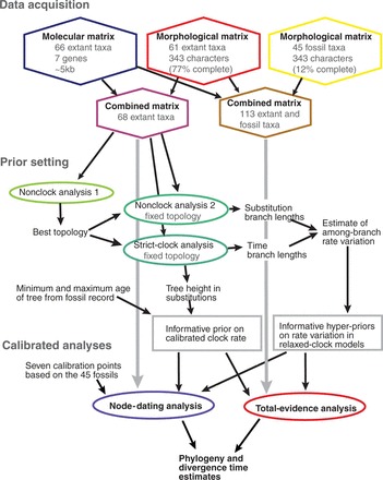
Figure 1. — Flow-chart showing the main analyses conducted in this study. See Materials and Methods section for details, explanations, and justifications for the different steps.

Specifying Priors for Relaxed-Clock Parameters

Because we could demonstrate significant rate variation across the extant tree, we explored relaxed-clock models in addition to standard nonclock and strict-clock models. In particular, we implemented Bayesian Markov chain Monte Carlo (MCMC) sampling in MrBayes 3.2 under three relaxed-clock models: the Thorne–Kishino 2002 (TK02) model (Thorne and Kishino 2002); the compound Poisson process (CPP) model (Huelsenbeck et al. 2000); and the independent gamma rates (IGR) model, originally described as the “white noise” model (Lepage et al. 2007).

The TK02 model is a continuous autocorrelated model, in which the evolutionary rate changes continuously along the branches of the tree in a manner similar to Brownian motion on the log scale. In particular, the evolutionary rate at a node is modeled by a lognormal distribution. The mean (not the log of the mean) of this distribution is the rate at the ancestral node, while the variance is proportional to the time separating the nodes, measured in expected substitutions per site at the base rate of the molecular clock. The overall evolutionary rate of a branch is taken to be the arithmetic average of the ancestral and descendant rates multiplied by the base rate of the clock. The rate at the root of the tree is assumed to be the same as the base rate of the molecular clock, as is true also for the other relaxed-clock models. Note that our implementation, which is virtually identical to that in Thorne and Kishino (2002), differs slightly from an earlier version of the model (Thorne et al. 1998).

The CPP model is a discrete autocorrelated model, in which the rate is successively modified by rate multipliers thrown onto the tree according to a Poisson process. Specifically, the rate multipliers are drawn from a lognormal distribution with a log mean of 0.0, ensuring that the rate does not tend to increase or decrease over time. We preferred the lognormal distribution over the modified gamma distribution used originally in the CPP model (Huelsenbeck et al. 2000) for mathematical convenience. The rate of the Poisson process and the variance of the lognormal distribution of the rate multipliers are not identifiable parameters (Rannala 2002). We address this by fixing the variance of the lognormal, such that each event is expected to result in some substantial change in the evolutionary rate, and by applying a suitable hyperprior to the rate of the Poisson process.

The CPP model was originally used only for fixed trees (Huelsenbeck et al. 2000); our implementation appears to be the first that also samples across tree space. The strategy we use was developed independently but is similar to the approach used by Blanquart and Lartillot (2006, 2008) to sample across tree space for a CPP model where the stationary state frequencies vary across the tree. For details of the MCMC implementation, we refer to the source code of MrBayes 3.2 (http://sourceforge.net/projects/mrbayes/develop/).

The IGR model is a continuous uncorrelated model, in which the branch rates are drawn independently from the same gamma distribution (Lepage et al. 2007). The mean of the gamma is the same as, and the variance is proportional to, the length of the branch measured in expected substitutions per site at the base rate of the clock. The IGR model is similar to the uncorrelated gamma model and related independent-branch rate models (Drummond et al. 2006), but it is mathematically more elegant in that it truly lacks time structure: the expected variance in effective branch lengths (branch lengths measured in terms of the number of expected substitutions per site) for a given time interval is the same regardless of how that interval is broken into branches.

Relaxed-Clock Prior Parameters

Relaxed-clock models are sensitive to the choice of priors, and we therefore exercised particular care in modeling rate variation appropriately (Fig. 2). To do this, we first found the nonclock topology with the highest posterior probability, which agreed well with previous studies of basal hymenopteran relationships and the papers cited therein(Heraty et al. 2011; Sharkey et al. 2011). We then sampled the branch length posteriors on this topology both under a nonclock and a strict-clock model. The ratio between the nonclock and strict-clock branch lengths gives a raw estimate of the branch rate that does not include a rate-smoothing component. Therefore, the variation of raw branch rates should provide a good guide for setting the hyperpriors in the rate-smoothing relaxed-clock models.

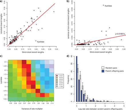
Figure 2. — Finding suitable prior parameters for relaxed-clock models. a) Relationship between branch lengths estimated under a strict-clock and under a nonclock model. The outlier corresponds to the branch leading to Xyelidae. b) Increase in variance (squared deviation from the expectation) of nonclock branch lengths over time. The slope of the regression line was used directly to center the prior for the variance increase parameter of the IGR model, and via simulations for the TK02 (Thorne–Kishino 2002) anc CPP models. c) Outcome of the simulations under the CPP model showing success of different combinations of the variance of the rate multiplier and the rate of the Poisson process to approximate the observed variance in branch lengths. Colors (in the online version of this figure) represent the relative deviation from the observed variance. The results were used to choose appropriate priors. d) The rate ratios observed in random pairs of branches tend to be higher than the ratios between parent and offspring pairs, demonstrating slight but significant rate autocorrelation in the data set (P=0.0055; Kolmogorov–Smirnov test of equality of distributions). The bars on the random pairs represent SDs obtained from 1000 replicates of random pair sets of the same size as the parent–offspring pair set.

The ratio between nonclock and strict-clock branch lengths was evenly distributed around the 1:1 expectation (Fig. 2a), and the variance (squared deviation from the 1:1 expectation) in nonclock branch lengths increased over time as expected (Fig. 2b). The IGR model assumes that the variance in effective branch lengths increases linearly over time. Therefore, we used the slope of the linear regression as the median for an exponential hyperprior on the variance increase parameter of this model.

For both the TK02 and the CPP model, we performed simulations in R (R Development Core Team 2009) in order to obtain suitable priors for the rate variation (R scripts provided as Supplementary Material). In the TK02 model, a single parameter controls the variation of the rate across the tree. Simulating the changes in evolutionary rates across our tree for different values of this parameter, we obtained an estimate of the optimal value. We used this estimate as the median of an exponential hyperprior on the variance parameter of the TK02 model.

In the CPP model, the variation in evolutionary rate depends on two parameters: the rate of the Poisson process generating rate multipliers, and the variance of the rate multipliers. To find parameter combinations resulting in the right amount of rate variation, we compared the variance of simulated effective branch lengths from the CPP model on our strict-clock tree to that of the nonclock branch lengths. The results show the expected inverse relationship between the rate and variance parameters of the CPP model (Fig. 2c). Any parameter combination along the optimal line would be appropriate for our analysis. We arbitrarily fixed the variance of the rate multipliers to a relatively high value (0.8), resulting in an expectation of a smaller number of more substantial rate-changing events. This is advantageous both from a parsimony perspective (fewer events needed to explain the rate variation) and in terms of MCMC convergence (CPP space with fewer events to sample across). To match this variance value, we then used an exponential hyperprior with mean 1.0 for the rate of the Poisson process (Fig. 2c).

In order to examine autocorrelation in rates across the tree, we compared the ratio of branch rates of parent–offspring pairs to the ratio of random pairs of branches (Fig. 2d). There was a small but significant tendency for parent–offspring pairs to have more similar rates (D=0.1625, P=0.0055; Kolmogorov–Smirnov test of equality of distributions). However, this observation does not mean that an autocorrelated relaxed-clock model necessarily has a better fit to our data, as this will depend on the actual distribution of rates across branches, and not only on the presence of some significant autocorrelation. Actually, the fact that the correlation was rather weak implies that parts of the tree could show no rate autocorrelation at all, a situation which could be difficult to model with one of our autocorrelated relaxed-clock models. We thus proceeded with all three relaxed-clock models and used Bayesian model choice to distinguish between them (see below).

Node Dating and Total-Evidence Dating

To obtain calibration points for the node-dating method, we assigned fossils to particular well-supported nodes of the tree of the extant taxa, relying on prior knowledge of their morphology and phylogenetic relationships. This resulted in seven calibration points within Hymenoptera Table 3 and Fig. 3, calibration points C–I; Rasnitsyn 1975; Rasnitsyn et al. 2003; Rasnitsyn and Zhang 2004; Zhang 1985; Zhang and Rasnitsyn 2007). It was not possible to extract more than seven calibration points out of the 45 fossil taxa included in our data set because many fossils were assigned to the same branches in the tree, or could not be assigned with certainty to any branch at all. In addition, we used two calibration points outside the Hymenoptera: one for Neoptera (calibration point A; same as the root of the tree; Prokop and Nel 2007) and one for Holometabola (calibration point B). All calibration nodes were fixed to be monophyletic, which appears justified given that they obtained 1.0 posterior probability in the nonclock analysis (Fig. 3). As a probability distribution on the age of each calibration node, we used an offset-exponential distribution with the minimum set to the age of the oldest fossil assigned to one of the subclades subtended by the node, and the mean set to the minimum age of a relevant calibration node pertaining to a more inclusive taxon (see Table 2 for details).

Table 3.

Fossils used in the node-dating analyses and calibration point prior settings

Calibration point	Prior on age (Ma)	Fossil(s)	Reference	PP correct^a (%)
A. Neoptera	min: 315	Katerinka (oldest Neoptera)	Prokop & Nel 2007
	mean: 396	Rhyniognatha (oldest insect)	Engel & Grimaldi 2004
B. Holometabola	min: 302	insect gall (oldest Holometabola)	Labandeira & Philips 1996
	mean: 396	Rhyniognatha	Engel & Grimaldi 2004
C. Hymenoptera	min: 235	Triassoxyela, Asioxyela	Rasnitsyn & Quicke 2002	96
	mean: 302	insect gall	Labandeira & Philips 1996
D. Xyelidae^b	min: 180	Eoxyela	Rasnitsyn 1983	0
E. Pamphilioidea^b	min: 161	Aulidontes, Pamphilidae undescribed	Rasnitsyn & Zhang 2004	48
F. Siricoidea^b	min: 161	Aulisca, Anaxyela, Syntexyela, Kulbastavia, Brachysyntexis	Zhang & Rasnitsyn 2006	0
G. Vespina^b	min: 180	Brigittepteris	Rasnitsyn et al. 2003	7
H. Apocrita^b	min: 176	Cleistogaster	Rasnitsyn 1975	34
I. Tenthredinoidea s.str.^b,^c	min: 140	Palaeathalia	Zhang 1985	100

Open in a new tab

The minimal and mean age for the offset-exponential prior are given, along with the corresponding fossils and references.

^aNotes: PP as obtained from the total-evidence analysis that the fossil attaches at the position assumed for the node-dating analysis. Note that these PPs take both the morphological data and the ages of the fossils into account.

^bThe mean age for all intra-hymenopteran calibration points was assumed to be the minimal age of Hymenoptera, i.e., 235 Ma (Triassoxyela, Asioxyela).

^cTenthredinoidea excluding Blasticotomidae.

Figure 3. — Phylogeny of extant Hymenoptera and outgroups retrieved under a nonclock model. Branch colors indicate the families of symphytans (the basal grade of Hymenoptera) included in the analysis. Capital letters followed by a star show the nine calibration points used in the calibrated analyses (Table 2). Values above nodes indicate Bayesian posterior probabilities.

In the total-evidence analysis, we removed all node calibrations except the root calibration (A) and the Holometabola calibration (B). A root calibration is required by the uniform tree prior, and the Holometabola calibration was retained because we included no outgroup fossils that could help date this part of the tree. All other calibration points were removed, and the corresponding nodes were no longer fixed to be monophyletic. The fossils were treated as terminals, with the age of each fossil fixed to the estimated age of the bed from which it was retrieved (Table 3). We did not attempt to accommodate the uncertainty in the dating of the fossil beds, since this is likely to be negligible compared to the other sources of error in the analysis.

To find an appropriate prior for the substitution rate (the base rate of the clock) in the calibrated analyses, we first ran uncalibrated strict-clock analyses with three different priors on tree height, namely exponential distributions with means of 0.1, 1.0, and 10. The posterior distribution on tree height was almost invariant across these prior settings, with the median ranging from 0.3326 to 0.3341. In deriving the base rate of the clock, we used the posterior distribution from the Exp(1.0) prior.

The outgroups in our analysis included a broad sample across Holometabola and some hemimetabolous Neoptera; therefore, reasonable estimates of the minimum and mean age of the tree might be the ages of Katerinka, the oldest fossil neopteran (Prokop and Nel 2007), and Rhyniognatha, the oldest insect (Engel and Grimaldi 2004). Dividing the median tree height with the mean age results in an estimated clock rate of ∼8.412×10⁻⁴ substitutions per site per million years, which was used as the mean of a lognormal prior on the clock rate. The standard deviation (SD) of the lognormal was chosen such that a rate estimate obtained by dividing the upper 95% estimate of the tree height by the age of Neoptera was removed by 1SD from the mean of the lognormal.

To assess the sensitivity of node age estimates to calibration settings, we also used a more restrictive and a less restrictive prior on the root calibration (A) and the Holometabola calibration (B). To obtain these priors, we doubled and halved the respective intervals between the minimum and mean of the offset-exponential distributions (Table 3).

Bayesian MCMC Analyses

To validate the implementation of the relaxed-clock models, the tree prior for total-evidence dating, and other aspects of the Bayesian MCMC machinery, we ran a number of tests that are available in the public SVN repository of MrBayes (https://mrbayes.svn.sourceforge.net/projects/mrbayes/develop) in the “test” directory. The tests included runs on simulated data to verify that we could retrieve parameter values correctly, and runs without data to check that we obtained reasonable samples from the prior distribution. We show an example from one of the latter tests here (Fig. 4). In this test, we used a data set consisting of either four extant terminals (Fig. 4a,c) or two extant terminals and two fossil terminals (Fig. 4b,d). In both cases, we could retrieve the tree probabilities (Fig. 4a,b) and the branch length distributions (Fig. 4c,d) with good precision.

Figure 4. — Extensive simulations were used to validate the MCMC algorithms. Here we show a simple example: retrieval of the uniform clock tree prior for a tree with four extant taxa a and c) and a tree with two extant taxa and two extinct taxa b and d). The age of the tree root was fixed to 1.0 in both cases, and the age of the fossils to 0.5. Both tree probabilities a and c) and branch length distributions b and d; only part shown in d) closely match analytically derived values. The results shown are for the strict-clock model; similar results were obtained under all relaxed-clock models.

To generate samples from the posteriors, we used four independent runs of four parallel chains each (MrBayes command blocks for all analyses are provided as Supplementary Material). The initial heating coefficient was set to 0.1, but lowered to 0.05 when the analyses included fossils to obtain chain swap probabilities between 10% and 40%. We used random starting trees, and sampled parameters and trees every 1000 generations. Analyses were run between 5 and 20 M generations, depending on the difficulty of getting convergence, at the High Performance Computing Center North in Umeå (http://www.hpc2n.umu.se). Convergence was assessed by the built-in diagnostics of MrBayes 3.2: the average SD of split frequencies (ASDSF; target value 0.05), the potential scale reduction factor (PSRF; target value 1.02), and the estimated sample size (ESS; target value 100). We also examined trace plots of likelihoods, chain swap frequencies, and parameter samples for evidence of non-stationarity or poor mixing. Burn-in was usually set to 25% of samples, but occasionally up to 50% of samples were discarded in difficult analyses. The diagnostic criteria were met for all parameters in all analyses except as noted below for the CPP model.

Bayes factors were used to choose among relaxed-clock models. They were calculated from estimates of the marginal likelihoods obtained using the stepping stone sampling approach (Xie et al. 2011), which we implemented in MrBayes 3.2. Our implementation estimates model likelihood by going from posterior to prior or in the reverse direction. It supports multiple-run convergence diagnostics, implements both initial and stepwise burn-in, and uses Metropolis coupling to enhance mixing during the entire procedure. The estimates presented here were based on an initial run of 20 M generations on the posterior, followed by 30 steps with 1000 samples obtained within each step (α=0.4). In total we ran 50 M generations, sampling every 1000 generations, and discarding 25% of the initial posterior samples, and the first 25% samples of each step, as burn-in.

Results

Tree Topology under Different Clock Models

The consensus tree obtained in an initial nonclock analysis of the combined extant data set (Fig. 3) is largely in agreement with previous hypotheses about inter-familial and inter-generic relationships in Hymenoptera (Heraty et al. 2011; Schulmeister 2003; Sharkey, 2007; Sharkey et al. 2011; Vilhelmsen et al. 2010; Vilhelmsen 2001). Most of the basal nodes received maximal support from the combined data set, posterior probability (PP) of 1.0, and were also recovered in analyses of morphology or molecules alone. Regions of uncertain resolution mainly include Tenthredinidae and Apocrita; the latter was very sparsely sampled. Additionally, the relationships at the base of Unicalcarida remain uncertain, especially whether Xiphydria is the sister to Vespina or to Siricidae.

The nonclock tree also shows that the rate of molecular evolution varies considerably between hymenopteran lineages, most conspicuously exemplified by the very short branches leading to extant Xyeloidea (Fig. 3). The Xyeloidea form the sister group of all other extant Hymenoptera in our analysis; previous studies have always placed the two constituent lineages, the Xyelinae and Macroxyelinae, at the very base of the hymenopteran tree, but variously as: a monophyletic group (Schulmeister 2003; Vilhelmsen 2001); as two separate lineages, each being the sister group of a large clade of other hymenopterans (Rasnitsyn 1988); as a basal grade with other hymenopterans monophyletic (Ronquist et al. 1999); or as unresolved (Sharkey 2002; Vilhelmsen 1997). The Xyeloidea have apparently retained many primitive characters found in the oldest known hymenopteran fossils (Rasnitsyn 2006). Our results show that the Xyeloidea are characterized by low evolutionary rates both in morphological and molecular characters.

The choice of clock model and rooting method had a large impact on tree topology (Fig. 5). The nonclock topology (Fig. 5b) agrees well with previous studies, including intuitively constructed morphology-based trees, and is identical to that obtained from only morphological characters (Fig. 5a), except for the placement of Syntexis within versus outside Siricoidea. Imposing a strict clock drastically changed the topology, most importantly by shuffling the outgroups and rerooting the hymenopteran tree on the branch separating the Vespina from other hymenopterans (Fig. 5c). Constraining the Holometabola to be monophyletic, to help structure outgroups according to the received wisdom, did not reverse the unorthodox rooting of the hymenopteran tree (Fig. 5d). Unconstrained relaxed-clock models similarly resulted in an unorthodox topology (Fig. 5e), but when the Holometabola constraint was added to help guide the rooting of the tree, the topological artifacts disappeared completely (Fig. 5f). All subsequent analyses used relaxed-clock models with the Holometabola constrained to be monophyletic.

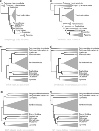
Figure 5. — Clock model and rooting assumption had a large effect on tree topology. When a clock was not assumed, the morphological a), molecular (not shown), and combined morphological and molecular b) trees were virtually congruent and agreed well with previous studies. c) Under the strict-clock model, however, the topology changed dramatically. d) Enforcing Holometabola to be monophyletic did not change hymenopteran relationships in the strict-clock analysis. e) The relaxed-clock models (here IGR) also produced apparent topological artifacts close to the root of the tree. f) When aided by a rooting constraint (Holometabola monophyletic), however, the relaxed-clock models (here IGR) retrieved the expected topology. The widths of clades are proportional to their representation in our data set, not to their true diversity. Only extant taxa were included in the analyses shown here.

Choosing a Relaxed-Clock Model

To select the best relaxed-clock model, we performed Bayes factor comparisons. Because the dating approach could influence the results, we performed the comparisons separately on the uncalibrated, node-calibrated, and total-evidence-calibrated data sets. Model likelihoods were computed using the stepping-stone algorithm (Xie et al. 2011), augmented by discarding a burn-in for each step to remove any temperature lag. Four independent analyses were performed on each data set.

The results differed across data sets. For the uncalibrated and node-calibrated data sets, the comparison favored the autocorrelated models (CPP and TK02) over the IGR model (CPP vs. IGR log Bayes factor ln F=21 and ln F=26 for the uncalibrated and calibrated analyses, respectively). The CPP model was slightly ahead of the TK02 model (ln F=5 and ln F=6, respectively).

For the total-evidence data set, we had some difficulties with convergence among the four independent stepping-stone analyses. The scatter among estimates was about 10 to 15 log likelihood units (except for TK02, see below), whereas it was around 5 log likelihood units for the other data sets. However, the results do suggest that inclusion of the fossils changed the performance of the models. In particular, the IGR model performed much better, on par with the CPP model. In four independent analyses, the model likelihood estimates for these models completely overlapped; the ranges were (−66853 to −66839) and (−66853 to −66842) for the CPP and IGR models, respectively. The TK02 model trailed behind with a range of (−67121 to −66853) (including an obvious outlier at −67121).

Examining the uncalibrated trees estimated by the different relaxed-clock models (Fig. 6) revealed that there is a major difference in the basal part of the tree, where evolutionary rates vary considerably even between neighboring branches (cf. Fig. 3). The IGR model allows the changes in substitution rates on adjacent basal branches to be quite extreme, accounting for most of the rate variation in the whole tree (Fig. 6a). In some cases, rates are strongly decelerated on one branch and accelerated on its sister branch, for example, in the most basal xyelid branch and in the ancestor of all other Hymenoptera. The autocorrelated CPP and TK02 models have a smoothing effect, such that the rate changes occur more slowly and over a larger part of the basal tree (Fig. 6b). The result is that the time duration of many basal branches is extended. For the uncalibrated analyses in general, the choice of relaxed-clock model had only a small effect on the estimates of effective branch lengths but often a profound effect on the estimated time lengths of the branches (Fig. 6c–f), which are crucial in dating.

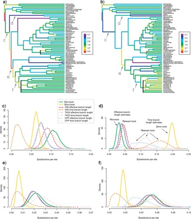
Figure 6. — Different relaxed-clock models result in different relative divergence time estimates (uncalibrated trees). a) Tree with branches colored according to their substitution rate as estimated under the IGR relaxed-clock model. The letters denote the branches examined in plots c–f, respectively. b) As previous, but under the CPP relaxed-clock model. c–f) Length of the four branches indicated in Figure 5a as estimated under different clock and nonclock models. For the relaxed-clock models, we plotted both the time length (in expected substitutions per site at the base rate of the clock) and the corresponding effective branch length, which equals the time length times the rate estimated for that branch (see labels in Fig. 5d). Note that effective branch lengths tend to be very similar to nonclock branch lengths, while time length distributions vary more across relaxed-clock models and tend to be less precise.

In the dated analyses, the extension of the basal branches resulted in the autocorrelated models implying the existence of considerably longer, unsampled ghost lineages than the IGR model, suggesting that the IGR model fits the fossil record better. Despite the fact that our tree model did not account for fossil sampling and thus did not penalize long ghost lineages, inclusion of the fossils in the analysis nevertheless tipped the model comparison in favor of the IGR model, as mentioned above, giving additional support for the idea that the IGR model agrees better with the fossil data. For these reasons, and because it also appears to us that it is more important to capture the apparently drastic rate changes among basal hymenopteran branches than it is to exactly model the rate autocorrelation in the rest of the tree, we focus on the IGR results in the following. Presumably, the rate variation in our data set would have been described more accurately by a relaxed-clock model allowing the degree of rate autocorrelation to change across the tree, unlike the models we explored.

Uncertainty in Fossil Placement

When fossils were included as terminals in the total-evidence analysis, the consensus tree was highly unresolved (Fig. 7). This is not surprising given the small number of morphological characters that could be scored for the fossils (4–20% depending on fossil preservation). The fossils that jump around in the tree mask any potential resolution among extant taxa in the consensus tree. When the consensus tree was calculated from the same tree sample after the fossil taxa were removed, the relationships among extant taxa were highly resolved and corresponded to the relationships obtained when analyzing extant taxa alone.

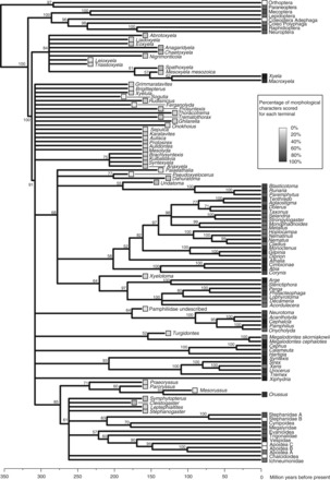
Figure 7. — Majority-rule consensus tree from a total-evidence analysis including all fossils (IGR model). The tree is poorly resolved, which reflects the uncertainty in fossil placement. The underlying consensus tree of extant taxa is virtually identical to trees obtained in analyses without fossils (see Figs. 7 and 8). Grey-scale boxes indicate the percentage of morphological characters that were coded for each taxon, showing the incompleteness of the fossils. Values above branches represent PPs.

The uncertainty concerning the phylogenetic placement varied considerably among the fossils. While some of the better preserved fossils could be assigned with high PP to a specific branch of the tree of extant taxa (e.g., Mesoxyela mesozoica, Fig. 8a), other fossils floated around over large parts of the tree. In some cases, this was apparently due to poor preservation (e.g., Sogutia liassica, only represented by a forewing impression, Fig. 8b), whereas in other cases, it seemed more likely due to the absence of apomorphic characters tying the fossils to any specific group (Fig. 8c,d).

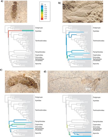
Figure 8. — The uncertainty in phylogenetic placement varied considerably across fossils. We show the PPs of four example fossils attaching to specific branches on the majority rule consensus tree of the extant taxa (IGR model). (a) *Mesoxyela mesozoica* Rasnitsyn, 1965 (140 Ma). (b) *Sogutia liassica* Rasnitsyn, 1977 (190 Ma). (c) *Aulisca odontura* Rasnitsyn, 1968 (161 Ma). (d) *Leptephialtities caudatus* Rasnitsyn, 1975 (161 Ma). Results were similar under the CPP and TK02 models.

Node Dating versus Total-Evidence Dating

Figure 9 shows the dated phylogeny obtained in the total-evidence analysis, with error bars on node ages from both total-evidence and traditional node dating. When comparing the age estimates, it is striking that all nodes outside Hymenoptera and in Xyelidae are estimated to be younger under the total-evidence approach, whereas the opposite is true for nodes within Hymenoptera excluding Xyelidae (arrows in Fig. 9). Furthermore, the variance of each estimate can differ considerably between the two approaches, usually being smaller in total-evidence dating (e.g., for the basal nodes in Hymenoptera) (Figs. 9 and 10). A striking exception is the age of the Xyelidae, where node dating leads to a much narrower (but probably erroneous; see below) age estimate.

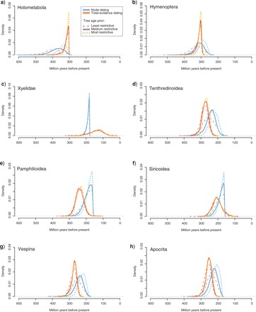
Figure 10. — Posteriors obtained under node dating and total-evidence dating are compared across three different priors on tree age for eight nodes (a–h; cf. Table 2). The nodes correspond to the most recent common ancestor of the extant forms of the specified taxa. For the intermediate prior on tree age, we used an offset-exponential distribution with a minimum of 315 Ma (oldest neopteran fossil) and a mean of 396 Ma (oldest insect fossil). For the more and less restrictive prior, we shifted the mean to half and twice the distance to the minimum (355 Ma and 477 Ma), respectively. Note that the total-evidence posteriors are less sensitive to prior assumptions than node-dating posteriors. They also tend to be more precise; if not, the total-evidence analysis indicated that the calibration points were based on erroneous or doubtful assumptions about fossil placement, causing posteriors to be artificially truncated (c; probably also e and f).

To study the precision and robustness of the age estimates, we varied the offset exponential prior distribution on the root age of the tree by doubling or halving its mean. This comparison shows that the total-ev idence approach is less sensitive to prior choice than the node-calibration approach (Fig. 10). The posterior also tends to be more precise. The exceptions (Fig. 10c,e,f) involve cases where the total-evidence analysis suggests that the relevant node calibration is based on erroneous or doubtful assumptions about the position of the crucial fossil, causing artificially narrow posteriors in the node-dating approach. Specifically, the total-evidence analysis showed that the PP of the critical fossil being correctly placed was <50% for four of the seven hymenopteran calibration points (Table 3). A prominent example is the Xyelidae calibration, mentioned above, which was based on the fossil Eoxyela tugnuica. This fossil shows some characteristics suggesting that it is closely related to extant species of Xyela (Rasnitsyn 1983), a placement that reached 0% PP in our analysis. Instead, Eoxyela is probably a stem-line xyelid (96% PP). This conflict in the placement of the calibration-point fossil is reflected in the node-dating analysis by an artificially narrow posterior distribution on the Xyelidae age, pushed towards the minimum age constraint (Fig. 10c).

Discussion

Relaxed-Clock Models

In many ways, relaxed-clock models are intermediate between strict-clock and nonclock models (Drummond et al. 2006). For instance, relaxed-clock models use much fewer parameters (roughly half as many) as nonclock models, but slightly more parameters than strict-clock models. They account for rate variation across lineages, unlike strict-clock models, but not as well as nonclock models. They provide weaker signal on the position of the root than strict-clock models, but stronger than nonclock models, which convey no rooting information at all.

In theory, relaxed-clock models could provide more precise and accurate phylogenetic results than either the strict-clock or nonclock models if they strike a better balance between model complexity (number of parameters) and model adequacy (accommodating rate variation across lineages) (Drummond et al. 2006). However, a recent simulation study has shown that this might not always be the case in practice (Wertheim et al. 2010), and our results support this conclusion. As expected, we observed topological artifacts under the strict-clock model, but most of these artifacts remained under the relaxed-clock models (Fig. 5), even when their priors were calibrated to accommodate the expected rate variation across the tree (Fig. 2).

These topological artifacts would presumably have disappeared if the rate smoothing effect of the relaxed-clock priors had been decreased. However, this would have removed much of the information about the position of the root and the time length of the branches, making it very challenging to date the tree. Because most of the rate variation in our data set was due to a few major rate changes, such an approach would probably also have resulted in exaggerated uncertainty in the dating of the bulk of the tree.

Rather than over-relaxing the clock, we chose to introduce a topological constraint close to the root of the tree to provide additional rooting information. Our results show that such a rooting constraint, on its own, can help relaxed-clock models pinpoint relevant rate changes close to the root and correct topological artifacts. The fact that the Holometabola constraint alone is sufficient to make all relaxed-clock models retrieve the expected topology (Fig. 5) also strengthens our supposition that this topology is indeed close, if not identical, to the true phylogenetic relationships. Of course, rooting constraints introduced in relaxed-clock analyses should be well justified. Few entomologists are likely to doubt the monophyly of Holometabola, which is supported by a large body of ontogenetic, ecological, and molecular evidence (Beutel et al. 2011; Hennig 1981; Kjer 2004; Kristensen 1999; Whiting et al. 1997).

It has been pointed out in the literature that both strict and relaxed-clock models could, in principle, be used to root phylogenetic trees without introducing outgroup constraints (Huelsenbeck et al. 2002; Renner et al. 2008). However, such rooting can be misled by model misfit, especially for strict-clock models (Huelsenbeck et al. 2002); by unbalanced sampling of in- and outgroups, which can be problematic for both strict- and relaxed-clock models; and by rate variation in general, which can be difficult to model correctly if it is concentrated around the root of the tree. Our results demonstrate several of these problems and exemplify the strength of the outgroup rooting method, even in the context of relaxed-clock models.

It is interesting to note that, despite their superficial similarity, there are clear differences among the three relaxed-clock models we explored in the estimated time tree. Even more interesting is the fact that their adequacy, as evidenced by Bayes factor comparisons, is influenced by the inclusion of fossils. Apparently, it is the presence of a few major rate changes close to the root of the hymenopteran tree that causes the major differences between the estimated time trees. As far as we can judge, this part of the tree is modeled best by the uncorrelated IGR model, which allows drastic rate variation among adjacent branches, whereas the autocorrelated CPP and TK02 models do better in the rest of the tree, where there is significant rate autocorrelation. Without fossils, the overall rate autocorrelation seems to determine the outcome of the model comparison, whereas inclusion of the fossils puts more emphasis on model adequacy in the basal part of the tree. An observation that seems to support these conclusions is that the CPP model performs better than the TK02 model across all data sets. In the CPP model, rate multipliers are thrown onto the tree according to a Poisson process. Although this is an autocorrelated model, it takes only one extreme multiplier, or a combination of a few multipliers, to generate more abrupt changes in evolutionary rate than would be expected in the gradual, continuous TK02 model of rate variation.

Morphological Clock

In total-evidence dating, the phylogenetic position of a fossil and the time duration of the branch connecting it to the extant tree are determined based on morphological evidence. The more similar a fossil is to the inferred morphology of an ancestor in the extant tree, and the more complete it is, the more it will influence the dating of the extant tree. The quantification of these ideas relies on the existence of a “morphological clock” (Ronquist, 1999; Lewis, 2001; Polly, 2001), which at first seems like a controversial proposition. In fact, however, all dating using fossils is based to some extent on the assumption that morphological similarity indicates temporal proximity. Even the most ardent opponents of the idea would have to agree that the fundamental assumption of morphological phylogenetic inference, descent with modification, implies that there is some correlation between morphological change and time. Of course, the rate of the morphological clock is likely to vary considerably over time and over characters (cf. Supplementary Figure 1), and there are likely to be complex dependencies between the evolutionary rates of different morphological characters. Nevertheless, we argue that it is better to attempt to explicitly quantify the morphological clock evidence, even if based on incomplete and over-simplified models of morphological evolution, than it is to use the evidence implicitly in constructing probability distributions for the age of calibration nodes.

An interesting question is whether the variation in evolutionary rates across the tree should be modeled jointly or separately for morphological and molecular data (Pyron 2011). We chose to model the rate variation jointly for several reasons. First, nonclock analyses showed that rate variation across the tree was clearly correlated across morphological and molecular partitions (see Supplementary Material). This was particularly obvious in the Xyeloidea, a clade that was characterized by extremely slow rates of both morphological and molecular evolution, but it appeared in many other parts of the tree as well. Second, our MCMC sampling was over effective branch lengths, and there would have been twice as many effective branch lengths (about 100 additional parameters) to sample over if rate variation had been modeled separately for morphology and molecules. We suspected it would be difficult to obtain convergence over such a large parameter space (see also Pyron 2011). Finally, modeling the rate variation separately could possibly also have resulted in problems related to over-parameterization. Nonetheless, we consider it worthwhile to further explore the separate modeling approach, especially for problems with fairly complete fossils and extensive morphological data.

Missing Data

Another concern under total-evidence dating is the impact of missing data. Ambiguous data entries are inevitably numerous for fossil taxa, which usually cannot be scored for any of the molecular characters. Especially when non-randomly distributed among taxa, such missing entries in the data matrix can interact with priors on topology and branch lengths in a way that could mislead tree reconstruction and divergence time estimation (Lemmon et al. 2009). On the other hand, such detrimental effects of missing data are probably weaker in the presence of a strong phylogenetic signal, and thus might have little impact when there is enough decisive data available (Lemmon et al. 2009; Wiens 2006; Wiens et al. 2010).

In our analyses, the addition of fossils had little impact on the topology recovered for extant taxa, suggesting that inferred relationships are not affected by missing data. But missing data could still affect branch length estimates, which are crucial for dating analyses. If so, then the least complete fossils should cause the most severe bias in estimated divergence times. However, when we excluded the most poorly preserved fossils (14 of the 45 fossils, those coded for <10% of the morphological data) from the total-evidence analysis, the recovered topology did not change and the median node ages were very similar to those obtained with the full set of fossils (Supplementary Figure 2). As expected, the confidence intervals of the divergence time estimates obtained with the reduced fossil set were usually wider, especially for those clades from which many fossils had been removed. This indicates that possible spurious effects caused by additional missing-data entries in the matrix are outweighed in our total-evidence dating analysis by the positive effects resulting from additional temporal information added by each fossil, however incompletely preserved.

Node Dating and Total-Evidence Dating

From a theoretical standpoint, total-evidence dating is preferable over standard node dating simply because it explicitly incorporates the fossil information instead of relying on secondary interpretation. We might also expect total-evidence dating to make more efficient use of the available data. The ideal case would be the dating of trees with poorly preserved fossils of uncertain affinity, which are difficult to use in node dating. However, such fossils might contain so little dating information that there is nevertheless little to gain from a total-evidence analysis.

Our results confirm that it is difficult to use the node-dating approach for hymenopteran dating because of the uncertainty in the placement of most fossils (Fig. 8). This is not surprising given the incompleteness of many of the fossil specimens, such as the single forewing remaining of Sogutia liassica (Fig. 8b). Despite these difficulties, however, the fossils contribute significantly to the dating of the tree in the total-evidence analysis. Compared to the node-calibration approach, the posterior distributions on divergence times are less sensitive to prior assumptions and also tend to be more precise in the total-evidence analysis (Fig. 10). Arguably, they also agree better with other dating studies, as discussed in detail below.

Perhaps more importantly, the total-evidence analysis highlighted several problems in the node-dating analysis. It showed that the PP of the critical fossil actually attaching in the predicted place on the extant tree was very low for no less than four of the seven Hymenoptera calibration points (Table 3). Such erroneous or biased node calibrations can lead to various problems in the inferred dates. For instance, the Xyelidae are estimated to be much older in the node-dating analysis than in the total-evidence analysis because the former assumes that the fossil Eoxyela tugnuica is positioned inside the Xyelidae. The total-evidence analysis, however, only assigns 2% PP to this placement, and instead suggests that Eoxyela is a stem-line xyelid (96% PP). The conflict between the hard lower bound on the age calibration of the Xyelidae and the branch length information from the phylogenetic model causes the posterior distribution on the xyelid age to be exceedingly narrow in the node-calibration analysis, pushed hard against the minimum age constraint.

Some of these artifacts can be avoided by using soft instead of hard bounds on the calibration ages (Yang and Rannala 2006). However, this assumes that it is possible to appropriately accommodate phylogenetic uncertainty in the calibration distributions, which appears more difficult to us than to actually incorporate the fossils in a total-evidence analysis. Alternative approaches to reconcile conflicting calibration points include compatibility and cross-validation analyses (Near et al. 2005; Near and Sanderson 2004; Rutschmann et al. 2007). However, these approaches tend to discard incompatible calibration points without considering the evidence supporting each one of them. In this and many other respects, they represent less powerful approaches than a true total-evidence analysis.

An interesting phenomenon is that our total-evidence analysis dated most nodes outside the Hymenoptera as younger, and most nodes inside the Hymenoptera as older, than the node-calibration analysis (Fig. 9). It is not entirely clear why, but it could partly be due to our tendency to place fossils inside extant groups, such as families, instead of fully considering the possibility that they belong to stem lineages further down in the tree. If so, this would help pull deep nodes towards the recent in the total-evidence analysis, where fossils find their position based on the available character evidence instead of on our ability to classify them correctly. However, it cannot explain why most Hymenoptera nodes are assigned older dates in the total-evidence analysis. This could possible be related to differences in the priors used for node dating and total-evidence dating.

Origin and Early Radiation of the Hymenoptera

The total-evidence analysis estimates the age of the order Hymenoptera to 309 Ma (95% credibility interval 291–347 Ma), and node dating leads to a very similar result (311 Ma, 95 credibility interval 257–369 Ma). This is considerably older than most previous estimates, which placed the origin in the Triassic e.g.,(Grimaldi and Engel 2005). In fact, our age estimate might seem unrealistically high given the known fossil record. For instance, it leaves a 74 myr gap to the first occurrence of Hymenoptera in the fossil record (Triassoxyela foveolata and Leioxyela antiqua at 235 Ma; Rasnitsyn 1964; Rasnitsyn and Quicke 2002). Furthermore, while our dating analysis places the major radiation of basal Hymenoptera in the Permian, most higher hymenopteran groups, including the Apocrita, are recorded for the first time only from the Lower Jurassic (Rasnitsyn 2010). The rather numerous hymenopteran fossils from the Triassic are currently all attributed to the Xyelidae (Rasnitsyn and Quicke, 2002).

Several factors could result in a bias toward too deep divergence times in our analyses. Over-estimation of node ages could be due to the relaxed-clock models being unable to accommodate the rate variation properly (Pulquério and Nichols 2007), or to the stochastic bias resulting from the fact that the evolutionary rate is likely to be a random variable with a strongly asymmetric distribution (Rondriguez-Trelles et al. 2002). In the node-dating analysis, incompatible calibration points could lead to too deep splits (Benton and Ayala 2003), and the same holds true for inappropriate modeling of morphological characters and possibly for the uniform tree prior in the total-evidence approach. Whether any of these mechanisms biased our results remains to be shown.

However, other lines of evidence suggest that our estimate might not be that unrealistic after all. First, the scarcity of hymenopteran fossils, especially in the early Jurassic, indicates that the order may be considerably older than the oldest fossils. Considering that the second oldest fossil at 190 Ma (Sogutia liassica; Rasnitsyn 1977) is separated by 45 myr from the oldest fossils, a gap of 74 myr between the oldest fossils and the origin of the order seems at least possible. Such major gaps in the fossil record are rather the rule than the exception in arthropods due to factors such as poor preservation, small size, limited distributional ranges, and a lack of attention from paleontologists (Wills 2001). In fact, even the best current fit of a Hymenoptera phylogeny to the fossil record contains a number of gaps in the range 85–140 myr (Rasnitsyn 2010). Furthermore, it is possible that the preponderance of xyelid fossils in the Triassic is due to the fact that other hymenopterans were less diverse and abundant during this time period. Another possibility is that some of the Triassic xyelids are actually unrecognized members of other basal hymenopteran lineages.

Accumulating evidence suggests that the Hymenoptera are the sister group of all other holometabolan insects (Beutel et al. 2011; Meusemann et al. 2010; Savard et al. 2006; Wiegmann et al. 2009). If so, and if hymenopterans radiated into extant lineages soon after their origin as suggested by our tree, then the age of the Hymenoptera should be close to the age of the Holometabola. The fossil record of several other holometabolous orders extends well into the Permian (Grimaldi and Engel 2005), suggesting that the Hymenoptera are at least this old. The oldest known fossil assigned to the Holometabola is a gall from the late Carboniferous, estimated to be ∼302 myr old. It could represent a hymenopterous gall, but this interpretation is rather controversial (Grimaldi and Engel 2005; Labandeira and Phillips 1996).

There is abundant additional evidence suggesting that the stem lineage of hymenopterans had separated from other Holometabola by the late Carboniferous (Rasnitsyn 1969, 1980, 2002; Rasnitsyn et al. 2004), agreeing well with our estimated divergence time for this split in the upper Carboniferous (Fig. 9). The fossil record indicates that there was a long period of evolution after that split, at least partly documented by the now extinct Palaeomanteida (= Miomoptera), before the Hymenoptera started radiating into extant lineages in the Triassic or Jurassic (Rasnitsyn 1980, 2002, 2010). It is here that our results differ by suggesting that the hymenopteran radiation started earlier, soon after the split from other holometabolans, leaving little room for a Palaeomanteida-like stem group. It should be borne in mind, however, that we did not include representatives of early holometabolans, such as the Palaeomanteida, in our study. A total-evidence analysis sampling more broadly across extant and extinct holometabolan lineages is needed before firm conclusions can be drawn on the time duration of the hymenopteran stem lineage and the role of the Palaeomanteida in the emergence of modern hymenopterans.

Regardless of the conclusion on the fit to the early hymenopteran fossil record, our results do agree well with a number of other dating studies. For instance, a recent supertree analysis (Davis et al. 2010), which compared fossil-based first occurrences of insect orders to phylogeny-based age estimates, found that many insect orders are likely to be considerably older than currently assumed. Specifically, the Hymenoptera were estimated to date back to the Carboniferous, ∼311 Ma, very close to our estimate of 309 Ma.

Age estimates for Hymenoptera based on molecular data are rather scarce. Wiegmann et al. (2009) used relaxed clock methods in combination with fossil calibration points to date the origin of holometabolan orders, obtaining an estimate of 350 Ma for the age of the Holometabola and 215–110 Ma for the basal split between three hymenopteran taxa, one of which was a tenthredinid. The latter is considerably younger than our estimate for the same split (304 Ma, 95% credibility interval 283–343 Ma), possibly due to the restricted sampling of hymenopteran taxa in Wiegmann et al.'s study leading to underestimation of branch lengths (Fitch and Bruschi 1987; Webster et al. 2003) and therefore biased age estimates. Other hymenopteran dating studies suggest that ants are at least 140 myr (Moreau 2011; Moreau et al. 2006) and bees at least 125 myr old (Danforth et al. 2006). These estimates agree better with our analysis, in which the ancestor of the rather scarcely sampled Vespoidea–Apoidea clade, including both bees and ants, is placed ∼170 Ma (95% credibility interval 123–225 Ma). In fact, our analysis suggests that the Apoidea, with the bees nested inside, dates back to ∼145 Ma, only 20 myr before the estimated time of radiation of extant bees at 125 Ma.

Conclusions

We conclude that, when feasible, total-evidence dating should be preferred over node dating. This is not only because total-evidence dating directly incorporates the evidence on which fossil dating is based instead of relying on indirect methods that may obscure or misrepresent the available data. Our study shows that total-evidence dating can also clearly outperform node dating when extracting information from poorly preserved fossils.

Moreover, the total-evidence approach provides a much better platform for future development of fossil dating. For instance, we can now start to directly explore models of speciation, extinction, sampling, and fossilization, and their effect on fossil dating of phylogenies, as a natural component of total-evidence analyses e.g.,(Stadler 2010). This would have been almost impossible within the framework of node dating.

Last but not least, the total-evidence approach puts the emphasis in fossil dating of phylogenies back where it belongs, in the empirical study of the fossil record. Our results clearly show that even with moderate amounts of molecular data, the uncertainty in effective branch lengths is negligible in comparison with the uncertainty in time lengths of branches (Fig. 6). Thus, increasing the sampling of molecular characters, which primarily are informative about effective branch lengths, will help little in improving divergence time estimates. Such improvements must instead come from more intense study of the fossils and their morphological characters, improved understanding of the nature of morphological evolution, better models of rate variation over time and across the tree, and more sophisticated priors for clock trees with fossils.

Supplementary Material

Supplementary material, including data files and online-only appendices, can be found in the Dryad data repository at http://datadryad.org, doi:10.5061/dryad.j2r64.

Funding

This work was supported by the Swedish Research Council [VR-2008-5629 to F.R.]; the National Science Foundation [DEB-0337220 to F.R. through the HymAToL project, PI Michael Sharkey]; and the Swiss National Science Foundation [PBBEP3_130173 to S.K.].

Acknowledgments

The authors contributed to this study as follows: F.R., L.V., A.P.R. and S.K. planned the study. L.V., S.S., A.P.R., and F.R. contributed to the definition of morphological characters and states, and L.V. and A.P.R. coded the missing extant and the fossil taxa for the morphological matrix. S.S., D.L.M., and S.K. contributed the molecular data. A.P.R. provided paleontological information and together with L.V. identified calibration points for the node-dating analysis. F.R. developed the models, priors, and Bayesian computational machinery. F.R. and S.K. planned the details of the analyses, analyzed the data, and wrote the manuscript. All authors revised the manuscript drafts, and read and approved the final manuscript.

We would like to thank Maxim Teslenko for implementing the stepping stone algorithm and providing crucial help with the programming, validation of algorithms, and analyses. We would also like to express our sincere gratitude to John Huelsenbeck, Bret Larget, Tom Britton, Sebastian Höhna, and Tanja Stadler for generously sharing ideas and commenting on various aspects of this study. A previous version of the manuscript was considerably improved by the extensive comments of Brian Moore and two anonymous reviewers.

References

Benton M.J., Ayala F.J. Dating the tree of life. Science. 2003;300:1698–1700. doi: 10.1126/science.1077795. [DOI] [PubMed] [Google Scholar]
Beutel R.G., Friedrich F., Hörnschemeyer T., Pohl H., Hünefeld F., Beckmann F., Meier R., Misof B., Whiting M.F., Vilhelmsen L. Morphological and molecular evidence converge upon a robust phylogeny of the megadiverse Holometabola. Cladistics. 2011;27:341–355. doi: 10.1111/j.1096-0031.2010.00338.x. [DOI] [PubMed] [Google Scholar]
Blanquart S., Lartillot N. A Bayesian compound stochastic process for modeling nonstationary and nonhomogeneous sequence evolution. Mol. Biol. E. 2006;23:2058–2071. doi: 10.1093/molbev/msl091. [DOI] [PubMed] [Google Scholar]
Blanquart S., Lartillot N. A site- and time-heterogeneous model of amino acid replacement. Mol. Biol. E. 2008;25:842–858. doi: 10.1093/molbev/msn018. [DOI] [PubMed] [Google Scholar]
Blum M., François O. Which random processes describe the tree of life? A large-scale study of phylogenetic tree imbalance. Syst. Biol. 2006;55:685–691. doi: 10.1080/10635150600889625. [DOI] [PubMed] [Google Scholar]
Danforth B.N., Ji S. Elongation factor-1 alpha occurs as two copies in bees: implications for phylogenetic analysis of EF1a sequences in insects. Mol. Biol. Evol. 1998;15:225–235. doi: 10.1093/oxfordjournals.molbev.a025920. [DOI] [PubMed] [Google Scholar]
Danforth B.N., Sipes S., Fang J., Brady S.G. The history of early bee diversification based on five genes plus morphology. Proc. Natl Acad. Sci. USA. 2006;103:15118–15123. doi: 10.1073/pnas.0604033103. [DOI] [PMC free article] [PubMed] [Google Scholar]
Davis R.B., Baldauf S.L., Mayhew P.J. Many hexapod groups originated earlier and withstood extinction events better than previously realized: inferences from supertrees. Proc. R. Soc. B Biol. Sci. 2010;277:1597–1606. doi: 10.1098/rspb.2009.2299. [DOI] [PMC free article] [PubMed] [Google Scholar]
Djernaes M., Damgaard J. Exon-intron structure, paralogy and sequenced regions of elongation factor-1 alpha in Hexapoda. Arthropod Syst. Phylogeny. 2006;64:45–52. [Google Scholar]
Dowton M., Austin A. Simultaneous analysis of 16S, 28S, COI and morphology in the Hymenoptera: Apocrita - evolutionary transitions among parasitic wasps. Biol. J. Linn. Soc. 2001;74:87–111. [Google Scholar]
Drummond A.J., Ho S.Y.W., Phillips M.J., Rambaut A. Relaxed phylogenetics and dating with confidence. PLoS Biol. 2006;4:e88. doi: 10.1371/journal.pbio.0040088. [DOI] [PMC free article] [PubMed] [Google Scholar]
Engel M.S., Grimaldi D.A. New light shed on the oldest insect. Nature. 2004;427:627–630. doi: 10.1038/nature02291. [DOI] [PubMed] [Google Scholar]
Fitch W.M., Bruschi M. The evolution of prokaryotic ferredoxins – with a general method correcting for unobserved substitutions in less branched lineages. Mol. Biol. Evol. 1987;4:381–394. doi: 10.1093/oxfordjournals.molbev.a040452. [DOI] [PubMed] [Google Scholar]
Grimaldi D.A., Engel M.S. Evolution of the insects. Cambridge, New York: Cambridge University Press; 2005. [Google Scholar]
Hennig W. Insect phylogeny. Chichester: John Wiley & Sons; 1981. [Google Scholar]
Heraty J., Ronquist F., Carpenter J.M., Hawks D., Schulmeister S., Dowling A.P., Murray D., Munro J., Wheeler W.C., Schiff N., Sharkey M. Evolution of the hymenopteran megaradiation. Mol. Phylogenet. Evol. 2011;60:73–88. doi: 10.1016/j.ympev.2011.04.003. [DOI] [PubMed] [Google Scholar]
Höhna S., Stadler T., Ronquist F., Britton T. Inferring speciation and extinction rates under different species sampling schemes. Mol. Biol. Evol. 2011;28:2577–2589. doi: 10.1093/molbev/msr095. [DOI] [PubMed] [Google Scholar]
Huelsenbeck J., Larget B., Swofford D. A compound Poisson process for relaxing the molecular clock. Genetics. 2000;154:1879–1892. doi: 10.1093/genetics/154.4.1879. [DOI] [PMC free article] [PubMed] [Google Scholar]
Huelsenbeck J.P., Bollback J.P., Levine A.M. Inferring the root of a phylogenetic tree. Syst. Biol. 2002;51:32–43. doi: 10.1080/106351502753475862. [DOI] [PubMed] [Google Scholar]
Kjer K.M. Aligned 18S and insect phylogeny. Syst. Biol. 2004;53:506–514. doi: 10.1080/10635150490445922. [DOI] [PubMed] [Google Scholar]
Kristensen N.P. Phylogeny of endopterygote insects, the most successful lineage of living organisms. Eur. J. Entomol. 1999;96:237–253. [Google Scholar]
Labandeira C.C., Phillips T.L. A Carboniferous insect gall: insight into early ecologic history of the Holometabola. Proc. Natl Acad. Sci. USA. 1996;93:8470–8474. doi: 10.1073/pnas.93.16.8470. [DOI] [PMC free article] [PubMed] [Google Scholar]
Lee M.S.Y., Oliver P.M., Hutchinson M.N. Phylogenetic uncertainty and molecular clock calibrations: a case study of legless lizards (Pygopodidae, Gekkota) Mol. Phylogenet. Evol. 2009;50:661–666. doi: 10.1016/j.ympev.2008.11.024. [DOI] [PubMed] [Google Scholar]
Lemmon A.R., Brown J.M., Stanger-Hall K., Moriarty Lemmon E. The effect of ambiguous data on phylogenetic estimates obtained by maximum likelihood and Bayesian inference. Syst. Biol. 2009;58:130–145. doi: 10.1093/sysbio/syp017. [DOI] [PMC free article] [PubMed] [Google Scholar]
Lepage T., Bryant D., Philippe H., Lartillot N. A general comparison of relaxed molecular clock models. Mol. Biol. Evol. 2007;24:2669–2680. doi: 10.1093/molbev/msm193. [DOI] [PubMed] [Google Scholar]
Lewis P.O. A likelihood approach to estimating phylogeny from discrete morphological character data. Syst. Biol. 2001;50:913–925. doi: 10.1080/106351501753462876. [DOI] [PubMed] [Google Scholar]
Linder M., Britton T., Sennblad B. Evaluation of Bayesian models of substitution rate evolution – parental guidance versus mutual independence. Syst. Biol. 2011;60:329–342. doi: 10.1093/sysbio/syr009. [DOI] [PubMed] [Google Scholar]
Manos P.S., Soltis P.S., Soltis D.E., Manchester S.R., Oh S.H., Bell C.D., Dilcher D.L., Stone D.E. Phylogeny of extant and extinct Juglandaceae inferred from the integration of molecular and morphological data sets. Syst. Biol. 2007;56:412–430. doi: 10.1080/10635150701408523. [DOI] [PubMed] [Google Scholar]
Marshall C.R. A simple method for bracketing absolute divergence times on molecular phylogenies using multiple fossil calibration points. Am. Nat. 2008;171:726–742. doi: 10.1086/587523. [DOI] [PubMed] [Google Scholar]
Matallón S. Using fossils to break long branches in molecular dating: a comparison of relaxed clocks applied to the origin of angiosperms. Syst. Biol. 2010;59:384–399. doi: 10.1093/sysbio/syq027. [DOI] [PubMed] [Google Scholar]
Meusemann K., von Reumont B.M., Simon S., Röding F., Strauss S., Kück P., Ebersberger I., Walzl M., Pass G., Breuers S., Achter V., von Haeseler A., Burmester T., Hadrys H., Wägele J. W., Misof B. A phylogenomic approach to resolve the arthropod tree of life. Mol. Biol. Evol. 2010;27:2451–2464. doi: 10.1093/molbev/msq130. [DOI] [PubMed] [Google Scholar]
Moreau C.S. What do molecular clocks tell us about the evolution of ants? (Invited instant symposium review) Am. Entomol. 2011;57:52–53. [Google Scholar]
Moreau C.S., Bell C.D., Vila R., Archibald S.B., Pierce N.E. Phylogeny of the ants: diversification in the age of angiosperms. Science. 2006;312:101–104. doi: 10.1126/science.1124891. [DOI] [PubMed] [Google Scholar]
Near T.J., Meylan P.A., Shaffer H.B. Assessing concordance of fossil calibration points in molecular clock studies: an example using turtles. Am. Nat. 2005;165:137–146. doi: 10.1086/427734. [DOI] [PubMed] [Google Scholar]
Near T.J., Sanderson M.J. Assessing the quality of molecular divergence time estimates by fossil calibrations and fossil-based model selection. Phil. T. R. Soc. B. 2004;359:1477–1483. doi: 10.1098/rstb.2004.1523. [DOI] [PMC free article] [PubMed] [Google Scholar]
Nylander J. A.A. MrModeltest v2 (Program distributed by the author). Uppsala, Sweden: Evolutionary Biology Centre, Uppsala University; 2004. [Google Scholar]
Parham J.F., Donoghue P.C., Bell C.J., Calway T.D., Head J.J., Holroyd P.A., Inoue J.G., Irmis R.B., Joyce W.G., Ksepka D.T., Patane J.S.L., Smith N.D., Tarver J.E., van Tuinen M., Yang Z., Angielczyk K.D., Greenwood J.M., Hipsley C.A., Jacobs L., Makovicky P.J., Müller J., Smith K.T., Theodor J.M., Warnock R.C.M., Benton M.J. Best practices for justifying fossil calibrations. Syst. Biol. 2012;61:346–359. doi: 10.1093/sysbio/syr107. [DOI] [PMC free article] [PubMed] [Google Scholar]
Polly P.D. On morphological clocks and paleophylogeography: towards a timescale forSorexhybrid zones. Genetica. 2001;112–113:339–357. [PubMed] [Google Scholar]
Prokop J., Nel A. An enigmatic Palaeozoic stem-group: Paoliida, designation of new taxa from the Upper Carboniferous of the Czech Republic (Insecta: Paoliidae, Katerinkidae fam. n.) Afr. Invertebr. 2007;48:77–86. [Google Scholar]
Pulquério M.J.F., Nichols R.A. Dates from the molecular clock: how wrong can we be? Trends Ecol. Evol. 2007;22:180–184. doi: 10.1016/j.tree.2006.11.013. [DOI] [PubMed] [Google Scholar]
Pyron R.A. Divergence time estimation using fossils as terminal taxa and the origins of Lissamphibia. Syst. Biol. 2011;60:466–481. doi: 10.1093/sysbio/syr047. [DOI] [PubMed] [Google Scholar]
Rannala B. Identifiability of parameters in MCMC Bayesian inference of phylogeny. Syst. Biol. 2002;51:754–760. doi: 10.1080/10635150290102429. [DOI] [PubMed] [Google Scholar]
Rasnitsyn A.P. New Triassic Hymenoptera of the Middle Asia (in Russian) Paleontol. Zh. 1964;1:88–96. [Google Scholar]
Rasnitsyn A.P. Origin and evolution of Lower Hymenoptera (in Russian) T. Paleontol. Inst. Acad. Sci. USSR. 1969;123:1–196. [Google Scholar]
Rasnitsyn A.P. Hymenoptera Apocrita of Mesozoic (in Russian) T. Paleontol. Inst. Acad. Sci. USSR. 1975;147:1–134. [Google Scholar]
Rasnitsyn A.P. Origin and evolution of Hymenoptera (in Russian) T. Paleontol. Inst. Acad. Sci. USSR. 1980;174:1–192. [Google Scholar]
Rasnitsyn A.P. Hymenopterous insects in Jurassic of the Eastern Siberia (in Russian) Bull. Moscow Soc. Nat. Biol. Sect. 1983;58:85–94. [Google Scholar]
Rasnitsyn A.P. An outline of evolution of the hymenopterous insects (order Vespida) Orient. Insects. 1988;22:115–145. [Google Scholar]
Rasnitsyn A.P. 2.2.1.3.1. Superorder Palaeomanteidea Handlirsch, 1906. Order Palaeomanteida Handlirsch, 1906. In: Rasnitsyn A.P., Quicke D.L.J., editors. History of insects. Dordrecht, Netherlands: Kluwer Academic Publishers; 2002. pp. 161–164. [Google Scholar]
Rasnitsyn A.P., Quicke D.L. History of insects. Dordrecht, Netherlands: Kluwer Academic Publisher; 2002. [Google Scholar]
Rasnitsyn A.P., Ansorge J., Zessin W. New hymenopterous insects (Insecta: Hymenoptera) from the Lower Toarcian (Lower Jurassic) of Germany. Neues Jahrb. Geol. P.–A. 2003;227:321–342. [Google Scholar]
Rasnitsyn A.P., Aristov D.S., Gorokhov A.V., Rowland J.M., Sinitshenkova N.D., Sukatsheva I.D. Important new fossil insects from Carrizo Arroyo and the Permo-Carboniferous faunal boundary. In: Lucas S.G., Ziegler K.E., editors. Carboniferous-Permian Transition. New Mexico Museum of Natural History and Science Bulletin 25. Albuquerque, New Mexico, USA: New Mexico Museum of Natural History and Science; 2004. pp. 215–246. [Google Scholar]
Rasnitsyn A.P., Zhang H. Composition and age of the Daohugou hymenopteran (Insecta, Hymenoptera = Vespida) assemblage from Inner Mongolia, China. Palaeontology. 2004;47:1507–1517. [Google Scholar]
Rasnitsyn A.P. Ontology of evolution and methodology of taxonomy. Paleontol. J. 2006;40:S679–S737. [Google Scholar]
Rasnitsyn A.P. Molecular phylogenetics, morphological cladistics, and fossil record. Entomol. Rev. 2010;90:263–298. [Google Scholar]
Renner S.S., Grimm G.W., Schneeweiss G.M., Stuessy T.E., Ricklefs R.E. Rooting and dating maples (Acer) with an uncorrelated-rates molecular clock: implications for North American/Asian disjunctions. Syst. Biol. 2008;57:795–808. doi: 10.1080/10635150802422282. [DOI] [PubMed] [Google Scholar]
Rondriguez-Trelles F., Tarrio R., Ayala F.J. A methodological bias toward overestimation of molecular evolutionary time scales. Proc. Natl Acad. Sci. USA. 2002;99:8112–8115. doi: 10.1073/pnas.122231299. [DOI] [PMC free article] [PubMed] [Google Scholar]
Ronquist F., Rasnitsyn A.P., Roy A., Eriksson K., Lindgren M. Phylogeny of the Hymenoptera: a cladistic reanalysis of Rasnitsyn's (1988) data. Zool. Scr. 1999;28:13–50. [Google Scholar]
Ronquist F., Teslenko M., van der Mark P., Ayres D.L., Darling A., Höhna S., Larget B., Liu L., Suchard M.A., Huelsenbeck J.P. MrBayes 3.2: efficient Bayesian phylogenetic inference and model choice across a large model space. Syst. Biol. 2012;61:539–542. doi: 10.1093/sysbio/sys029. [DOI] [PMC free article] [PubMed] [Google Scholar]
Ronquist F. Phylogeny, classification and evolution of the Cynipoidea. Zool. Scr. 1999;28:139–164. [Google Scholar]
Rutschmann F., Eriksson T., Abu Salim K., Conti E. Assessing calibration uncertainty in molecular dating: the assignment of fossils to alternative calibration points. Syst. Biol. 2007;56:591–608. doi: 10.1080/10635150701491156. [DOI] [PubMed] [Google Scholar]
R Development Core Team. R: a language and environment for statistical computing. Vienna, Austria: R Foundation for Statistical Computing; 2009. [Google Scholar]
Savard J., Tautz D., Richards S., Weinstock G.M., Gibbs R.A., Werren J.H., Tettelin H., Lercher M.J. Phylogenomic analysis reveals bees and wasps (Hymenoptera) at the base of the radiation of holometabolous insects. Genome Res. 2006;16:1334–1338. doi: 10.1101/gr.5204306. [DOI] [PMC free article] [PubMed] [Google Scholar]
Schulmeister S. Review of morphological evidence on the phylogeny of basal Hymenoptera (Insecta), with a discussion of the ordering of characters. Biol. J. Linn. Soc. 2003;79:209–243. [Google Scholar]
Sharkey M. Phylogeny of the Hymenoptera: a reanalysis of the Ronquist (1999) reanalysis, emphasizing wing venation and apocritan relationships. Zool. Scr. 2002;31:57–66. [Google Scholar]
Sharkey M. Phylogeny and classification of Hymenoptera. Zootaxa. 2007;1668:1–766. [Google Scholar]
Sharkey M.J., Carpenter J.M., Vilhelmsen L., Heraty J., Liljeblad J., Dowling A.P.G., Schulmeister S., Murray D., Deans A.R., Ronquist F., Krogmann L., Wheeler W.C. Phylogenetic relationships among superfamilies of Hymenoptera. Cladistics. 2011;27:1–33. doi: 10.1111/j.1096-0031.2011.00366.x. [DOI] [PubMed] [Google Scholar]
Stadler T. Sampling-through-time in birth-death trees. J. Theor. Biol. 2010;267:396–404. doi: 10.1016/j.jtbi.2010.09.010. [DOI] [PubMed] [Google Scholar]
Thorne J.L., Kishino H., Painter I.S. Estimating the rate of evolution of the rate of molecular evolution. Mol. Biol. Evol. 1998;15:1647–1657. doi: 10.1093/oxfordjournals.molbev.a025892. [DOI] [PubMed] [Google Scholar]
Thorne J.L., Kishino H. Divergence time and evolutionary rate estimation with multilocus data. Syst. Biol. 2002;51:689–702. doi: 10.1080/10635150290102456. [DOI] [PubMed] [Google Scholar]
Vilhelmsen L., Mikó I., Krogmann L. Beyond the wasp-waist: structural diversity and phylogenetic significance of the mesosoma in apocritan wasps (Insecta: Hymenoptera) Zool. J. Linn. Soc. 2010;159:22–194. [Google Scholar]
Vilhelmsen L. Phylogeny and classification of the extant basal lineages of the Hymenoptera (Insecta) Zool. J. Linn. Soc. 2001;131:393–442. [Google Scholar]
Vilhelmsen L. The phylogeny of lower Hymenoptera (Insecta), with a summary of the early evolutionary history of the order. J. Zool. Syst. Evol. Res. 1997;35:49–70. [Google Scholar]
Warnock R.C.M., Yang Z., Donoghue P.C.J. Exploring uncertainty in the calibration of the molecular clock. Biol. Lett. 2011 doi: 10.1098/rsbl.2011.0710. doi: 10.1098/rsbl.2011.0710. [DOI] [PMC free article] [PubMed] [Google Scholar]
Webster A.J., Payne R.J.H., Pagel M. Molecular phylogenies link rates of evolution and speciation. Science. 2003;301:478. doi: 10.1126/science.1083202. [DOI] [PubMed] [Google Scholar]
Wertheim J.O., Sanderson M.J., Worobey M., Bjork A. Relaxed molecular clocks, the bias-variance trade-off, and the quality of phylogenetic inference. Syst. Biol. 2010;59:1–8. doi: 10.1093/sysbio/syp072. [DOI] [PMC free article] [PubMed] [Google Scholar]
Whiting M.F., Carpenter J.C., Wheeler Q.D., Wheeler W.C. The Strepsiptera problem: phylogeny of the holometabolous insect orders inferred from 18S and 28S ribosomal DNA sequences and morphology. Syst. Biol. 1997;46:1–68. doi: 10.1093/sysbio/46.1.1. [DOI] [PubMed] [Google Scholar]
Wiegmann B.M., Trautwein M.D., Kim J.-W., Cassel B.K., Bertone M.A., Winterton S.L., Yeates D.K. Single-copy nuclear genes resolve the phylogeny of the holometabolous insects. BMC Biol. 2009;7:34. doi: 10.1186/1741-7007-7-34. [DOI] [PMC free article] [PubMed] [Google Scholar]
Wiens J.J. Missing data and the design of phylogenetic analyses. J. Biomed. Inform. 2006;39:34–42. doi: 10.1016/j.jbi.2005.04.001. [DOI] [PubMed] [Google Scholar]
Wiens J.J., Kuczynski C.A., Townsend T., Reeder T.W., Mulcahy D.G., Sites Jr J.W. Combining phylogenomics and fossils in higher level squamate reptile phylogeny: molecular data change the placement of fossil taxa. Syst. Biol. 2010;59:674–688. doi: 10.1093/sysbio/syq048. [DOI] [PubMed] [Google Scholar]
Wills M.A. How good is the fossil record of arthropods? An assessment using the stratigraphic congruence of cladograms. Geol. J. 2001;36:187–210. [Google Scholar]
Xie W., Lewis P.O., Fan Y., Kuo L., Chen M.-H. Improving marginal likelihood estimation for Bayesian phylogenetic model selection. Syst. Biol. 2011;60:150–160. doi: 10.1093/sysbio/syq085. [DOI] [PMC free article] [PubMed] [Google Scholar]
Yang Z., Rannala B. Bayesian estimation of species divergence times under a molecular clock using multiple fossil calibrations with soft bounds. Mol. Biol. E. 2006;23:212–226. doi: 10.1093/molbev/msj024. [DOI] [PubMed] [Google Scholar]
Zhang J. New data on the Mesozoic fossil insects from Laiyang in Shandong. Geol. Shandong. 1985;1:23–39. [Google Scholar]
Zhang H., Rasnitsyn A.P. Two anaxyelid sawflies (Insecta, Hymenoptera, Siricoidea) from the Yixian Formation of western Liaoning, China. Cretaceous Res. 2007;27:279–284. [Google Scholar]
Zuckerkandl E., Pauling L. Molecular disease, evolution and genetic heterogeneity. In: Kasha M., Pullman B., editors. Horizons in biochemistry. New York: Academic Press; 1962. pp. 189–225. [Google Scholar]

[B1] Benton M.J., Ayala F.J. Dating the tree of life. Science. 2003;300:1698–1700. doi: 10.1126/science.1077795. [DOI] [PubMed] [Google Scholar]

[B2] Beutel R.G., Friedrich F., Hörnschemeyer T., Pohl H., Hünefeld F., Beckmann F., Meier R., Misof B., Whiting M.F., Vilhelmsen L. Morphological and molecular evidence converge upon a robust phylogeny of the megadiverse Holometabola. Cladistics. 2011;27:341–355. doi: 10.1111/j.1096-0031.2010.00338.x. [DOI] [PubMed] [Google Scholar]

[B3] Blanquart S., Lartillot N. A Bayesian compound stochastic process for modeling nonstationary and nonhomogeneous sequence evolution. Mol. Biol. E. 2006;23:2058–2071. doi: 10.1093/molbev/msl091. [DOI] [PubMed] [Google Scholar]

[B4] Blanquart S., Lartillot N. A site- and time-heterogeneous model of amino acid replacement. Mol. Biol. E. 2008;25:842–858. doi: 10.1093/molbev/msn018. [DOI] [PubMed] [Google Scholar]

[B5] Blum M., François O. Which random processes describe the tree of life? A large-scale study of phylogenetic tree imbalance. Syst. Biol. 2006;55:685–691. doi: 10.1080/10635150600889625. [DOI] [PubMed] [Google Scholar]

[B6] Danforth B.N., Ji S. Elongation factor-1 alpha occurs as two copies in bees: implications for phylogenetic analysis of EF1a sequences in insects. Mol. Biol. Evol. 1998;15:225–235. doi: 10.1093/oxfordjournals.molbev.a025920. [DOI] [PubMed] [Google Scholar]

[B7] Danforth B.N., Sipes S., Fang J., Brady S.G. The history of early bee diversification based on five genes plus morphology. Proc. Natl Acad. Sci. USA. 2006;103:15118–15123. doi: 10.1073/pnas.0604033103. [DOI] [PMC free article] [PubMed] [Google Scholar]

[B8] Davis R.B., Baldauf S.L., Mayhew P.J. Many hexapod groups originated earlier and withstood extinction events better than previously realized: inferences from supertrees. Proc. R. Soc. B Biol. Sci. 2010;277:1597–1606. doi: 10.1098/rspb.2009.2299. [DOI] [PMC free article] [PubMed] [Google Scholar]

[B9] Djernaes M., Damgaard J. Exon-intron structure, paralogy and sequenced regions of elongation factor-1 alpha in Hexapoda. Arthropod Syst. Phylogeny. 2006;64:45–52. [Google Scholar]

[B10] Dowton M., Austin A. Simultaneous analysis of 16S, 28S, COI and morphology in the Hymenoptera: Apocrita - evolutionary transitions among parasitic wasps. Biol. J. Linn. Soc. 2001;74:87–111. [Google Scholar]

[B11] Drummond A.J., Ho S.Y.W., Phillips M.J., Rambaut A. Relaxed phylogenetics and dating with confidence. PLoS Biol. 2006;4:e88. doi: 10.1371/journal.pbio.0040088. [DOI] [PMC free article] [PubMed] [Google Scholar]

[B12] Engel M.S., Grimaldi D.A. New light shed on the oldest insect. Nature. 2004;427:627–630. doi: 10.1038/nature02291. [DOI] [PubMed] [Google Scholar]

[B13] Fitch W.M., Bruschi M. The evolution of prokaryotic ferredoxins – with a general method correcting for unobserved substitutions in less branched lineages. Mol. Biol. Evol. 1987;4:381–394. doi: 10.1093/oxfordjournals.molbev.a040452. [DOI] [PubMed] [Google Scholar]

[B14] Grimaldi D.A., Engel M.S. Evolution of the insects. Cambridge, New York: Cambridge University Press; 2005. [Google Scholar]

[B15] Hennig W. Insect phylogeny. Chichester: John Wiley & Sons; 1981. [Google Scholar]

[B16] Heraty J., Ronquist F., Carpenter J.M., Hawks D., Schulmeister S., Dowling A.P., Murray D., Munro J., Wheeler W.C., Schiff N., Sharkey M. Evolution of the hymenopteran megaradiation. Mol. Phylogenet. Evol. 2011;60:73–88. doi: 10.1016/j.ympev.2011.04.003. [DOI] [PubMed] [Google Scholar]

[B17] Höhna S., Stadler T., Ronquist F., Britton T. Inferring speciation and extinction rates under different species sampling schemes. Mol. Biol. Evol. 2011;28:2577–2589. doi: 10.1093/molbev/msr095. [DOI] [PubMed] [Google Scholar]

[B18] Huelsenbeck J., Larget B., Swofford D. A compound Poisson process for relaxing the molecular clock. Genetics. 2000;154:1879–1892. doi: 10.1093/genetics/154.4.1879. [DOI] [PMC free article] [PubMed] [Google Scholar]

[B19] Huelsenbeck J.P., Bollback J.P., Levine A.M. Inferring the root of a phylogenetic tree. Syst. Biol. 2002;51:32–43. doi: 10.1080/106351502753475862. [DOI] [PubMed] [Google Scholar]

[B20] Kjer K.M. Aligned 18S and insect phylogeny. Syst. Biol. 2004;53:506–514. doi: 10.1080/10635150490445922. [DOI] [PubMed] [Google Scholar]

[B21] Kristensen N.P. Phylogeny of endopterygote insects, the most successful lineage of living organisms. Eur. J. Entomol. 1999;96:237–253. [Google Scholar]

[B22] Labandeira C.C., Phillips T.L. A Carboniferous insect gall: insight into early ecologic history of the Holometabola. Proc. Natl Acad. Sci. USA. 1996;93:8470–8474. doi: 10.1073/pnas.93.16.8470. [DOI] [PMC free article] [PubMed] [Google Scholar]

[B23] Lee M.S.Y., Oliver P.M., Hutchinson M.N. Phylogenetic uncertainty and molecular clock calibrations: a case study of legless lizards (Pygopodidae, Gekkota) Mol. Phylogenet. Evol. 2009;50:661–666. doi: 10.1016/j.ympev.2008.11.024. [DOI] [PubMed] [Google Scholar]

[B24] Lemmon A.R., Brown J.M., Stanger-Hall K., Moriarty Lemmon E. The effect of ambiguous data on phylogenetic estimates obtained by maximum likelihood and Bayesian inference. Syst. Biol. 2009;58:130–145. doi: 10.1093/sysbio/syp017. [DOI] [PMC free article] [PubMed] [Google Scholar]

[B25] Lepage T., Bryant D., Philippe H., Lartillot N. A general comparison of relaxed molecular clock models. Mol. Biol. Evol. 2007;24:2669–2680. doi: 10.1093/molbev/msm193. [DOI] [PubMed] [Google Scholar]

[B26] Lewis P.O. A likelihood approach to estimating phylogeny from discrete morphological character data. Syst. Biol. 2001;50:913–925. doi: 10.1080/106351501753462876. [DOI] [PubMed] [Google Scholar]

[B27] Linder M., Britton T., Sennblad B. Evaluation of Bayesian models of substitution rate evolution – parental guidance versus mutual independence. Syst. Biol. 2011;60:329–342. doi: 10.1093/sysbio/syr009. [DOI] [PubMed] [Google Scholar]

[B28] Manos P.S., Soltis P.S., Soltis D.E., Manchester S.R., Oh S.H., Bell C.D., Dilcher D.L., Stone D.E. Phylogeny of extant and extinct Juglandaceae inferred from the integration of molecular and morphological data sets. Syst. Biol. 2007;56:412–430. doi: 10.1080/10635150701408523. [DOI] [PubMed] [Google Scholar]

[B29] Marshall C.R. A simple method for bracketing absolute divergence times on molecular phylogenies using multiple fossil calibration points. Am. Nat. 2008;171:726–742. doi: 10.1086/587523. [DOI] [PubMed] [Google Scholar]

[B30] Matallón S. Using fossils to break long branches in molecular dating: a comparison of relaxed clocks applied to the origin of angiosperms. Syst. Biol. 2010;59:384–399. doi: 10.1093/sysbio/syq027. [DOI] [PubMed] [Google Scholar]

[B31] Meusemann K., von Reumont B.M., Simon S., Röding F., Strauss S., Kück P., Ebersberger I., Walzl M., Pass G., Breuers S., Achter V., von Haeseler A., Burmester T., Hadrys H., Wägele J. W., Misof B. A phylogenomic approach to resolve the arthropod tree of life. Mol. Biol. Evol. 2010;27:2451–2464. doi: 10.1093/molbev/msq130. [DOI] [PubMed] [Google Scholar]

[B32] Moreau C.S. What do molecular clocks tell us about the evolution of ants? (Invited instant symposium review) Am. Entomol. 2011;57:52–53. [Google Scholar]

[B33] Moreau C.S., Bell C.D., Vila R., Archibald S.B., Pierce N.E. Phylogeny of the ants: diversification in the age of angiosperms. Science. 2006;312:101–104. doi: 10.1126/science.1124891. [DOI] [PubMed] [Google Scholar]

[B34] Near T.J., Meylan P.A., Shaffer H.B. Assessing concordance of fossil calibration points in molecular clock studies: an example using turtles. Am. Nat. 2005;165:137–146. doi: 10.1086/427734. [DOI] [PubMed] [Google Scholar]

[B35] Near T.J., Sanderson M.J. Assessing the quality of molecular divergence time estimates by fossil calibrations and fossil-based model selection. Phil. T. R. Soc. B. 2004;359:1477–1483. doi: 10.1098/rstb.2004.1523. [DOI] [PMC free article] [PubMed] [Google Scholar]

[B36] Nylander J. A.A. MrModeltest v2 (Program distributed by the author). Uppsala, Sweden: Evolutionary Biology Centre, Uppsala University; 2004. [Google Scholar]

[B37] Parham J.F., Donoghue P.C., Bell C.J., Calway T.D., Head J.J., Holroyd P.A., Inoue J.G., Irmis R.B., Joyce W.G., Ksepka D.T., Patane J.S.L., Smith N.D., Tarver J.E., van Tuinen M., Yang Z., Angielczyk K.D., Greenwood J.M., Hipsley C.A., Jacobs L., Makovicky P.J., Müller J., Smith K.T., Theodor J.M., Warnock R.C.M., Benton M.J. Best practices for justifying fossil calibrations. Syst. Biol. 2012;61:346–359. doi: 10.1093/sysbio/syr107. [DOI] [PMC free article] [PubMed] [Google Scholar]

[B38] Polly P.D. On morphological clocks and paleophylogeography: towards a timescale forSorexhybrid zones. Genetica. 2001;112–113:339–357. [PubMed] [Google Scholar]

[B39] Prokop J., Nel A. An enigmatic Palaeozoic stem-group: Paoliida, designation of new taxa from the Upper Carboniferous of the Czech Republic (Insecta: Paoliidae, Katerinkidae fam. n.) Afr. Invertebr. 2007;48:77–86. [Google Scholar]

[B40] Pulquério M.J.F., Nichols R.A. Dates from the molecular clock: how wrong can we be? Trends Ecol. Evol. 2007;22:180–184. doi: 10.1016/j.tree.2006.11.013. [DOI] [PubMed] [Google Scholar]

[B41] Pyron R.A. Divergence time estimation using fossils as terminal taxa and the origins of Lissamphibia. Syst. Biol. 2011;60:466–481. doi: 10.1093/sysbio/syr047. [DOI] [PubMed] [Google Scholar]

[B42] Rannala B. Identifiability of parameters in MCMC Bayesian inference of phylogeny. Syst. Biol. 2002;51:754–760. doi: 10.1080/10635150290102429. [DOI] [PubMed] [Google Scholar]

[B43] Rasnitsyn A.P. New Triassic Hymenoptera of the Middle Asia (in Russian) Paleontol. Zh. 1964;1:88–96. [Google Scholar]

[B44] Rasnitsyn A.P. Origin and evolution of Lower Hymenoptera (in Russian) T. Paleontol. Inst. Acad. Sci. USSR. 1969;123:1–196. [Google Scholar]

[B45] Rasnitsyn A.P. Hymenoptera Apocrita of Mesozoic (in Russian) T. Paleontol. Inst. Acad. Sci. USSR. 1975;147:1–134. [Google Scholar]

[B46] Rasnitsyn A.P. Origin and evolution of Hymenoptera (in Russian) T. Paleontol. Inst. Acad. Sci. USSR. 1980;174:1–192. [Google Scholar]

[B47] Rasnitsyn A.P. Hymenopterous insects in Jurassic of the Eastern Siberia (in Russian) Bull. Moscow Soc. Nat. Biol. Sect. 1983;58:85–94. [Google Scholar]

[B48] Rasnitsyn A.P. An outline of evolution of the hymenopterous insects (order Vespida) Orient. Insects. 1988;22:115–145. [Google Scholar]

[B49] Rasnitsyn A.P. 2.2.1.3.1. Superorder Palaeomanteidea Handlirsch, 1906. Order Palaeomanteida Handlirsch, 1906. In: Rasnitsyn A.P., Quicke D.L.J., editors. History of insects. Dordrecht, Netherlands: Kluwer Academic Publishers; 2002. pp. 161–164. [Google Scholar]

[B50] Rasnitsyn A.P., Quicke D.L. History of insects. Dordrecht, Netherlands: Kluwer Academic Publisher; 2002. [Google Scholar]

[B51] Rasnitsyn A.P., Ansorge J., Zessin W. New hymenopterous insects (Insecta: Hymenoptera) from the Lower Toarcian (Lower Jurassic) of Germany. Neues Jahrb. Geol. P.–A. 2003;227:321–342. [Google Scholar]

[B52] Rasnitsyn A.P., Aristov D.S., Gorokhov A.V., Rowland J.M., Sinitshenkova N.D., Sukatsheva I.D. Important new fossil insects from Carrizo Arroyo and the Permo-Carboniferous faunal boundary. In: Lucas S.G., Ziegler K.E., editors. Carboniferous-Permian Transition. New Mexico Museum of Natural History and Science Bulletin 25. Albuquerque, New Mexico, USA: New Mexico Museum of Natural History and Science; 2004. pp. 215–246. [Google Scholar]

[B53] Rasnitsyn A.P., Zhang H. Composition and age of the Daohugou hymenopteran (Insecta, Hymenoptera = Vespida) assemblage from Inner Mongolia, China. Palaeontology. 2004;47:1507–1517. [Google Scholar]

[B54] Rasnitsyn A.P. Ontology of evolution and methodology of taxonomy. Paleontol. J. 2006;40:S679–S737. [Google Scholar]

[B55] Rasnitsyn A.P. Molecular phylogenetics, morphological cladistics, and fossil record. Entomol. Rev. 2010;90:263–298. [Google Scholar]

[B56] Renner S.S., Grimm G.W., Schneeweiss G.M., Stuessy T.E., Ricklefs R.E. Rooting and dating maples (Acer) with an uncorrelated-rates molecular clock: implications for North American/Asian disjunctions. Syst. Biol. 2008;57:795–808. doi: 10.1080/10635150802422282. [DOI] [PubMed] [Google Scholar]

[B57] Rondriguez-Trelles F., Tarrio R., Ayala F.J. A methodological bias toward overestimation of molecular evolutionary time scales. Proc. Natl Acad. Sci. USA. 2002;99:8112–8115. doi: 10.1073/pnas.122231299. [DOI] [PMC free article] [PubMed] [Google Scholar]

[B58] Ronquist F., Rasnitsyn A.P., Roy A., Eriksson K., Lindgren M. Phylogeny of the Hymenoptera: a cladistic reanalysis of Rasnitsyn's (1988) data. Zool. Scr. 1999;28:13–50. [Google Scholar]

[B59] Ronquist F., Teslenko M., van der Mark P., Ayres D.L., Darling A., Höhna S., Larget B., Liu L., Suchard M.A., Huelsenbeck J.P. MrBayes 3.2: efficient Bayesian phylogenetic inference and model choice across a large model space. Syst. Biol. 2012;61:539–542. doi: 10.1093/sysbio/sys029. [DOI] [PMC free article] [PubMed] [Google Scholar]

[B60] Ronquist F. Phylogeny, classification and evolution of the Cynipoidea. Zool. Scr. 1999;28:139–164. [Google Scholar]

[B61] Rutschmann F., Eriksson T., Abu Salim K., Conti E. Assessing calibration uncertainty in molecular dating: the assignment of fossils to alternative calibration points. Syst. Biol. 2007;56:591–608. doi: 10.1080/10635150701491156. [DOI] [PubMed] [Google Scholar]

[B62] R Development Core Team. R: a language and environment for statistical computing. Vienna, Austria: R Foundation for Statistical Computing; 2009. [Google Scholar]

[B63] Savard J., Tautz D., Richards S., Weinstock G.M., Gibbs R.A., Werren J.H., Tettelin H., Lercher M.J. Phylogenomic analysis reveals bees and wasps (Hymenoptera) at the base of the radiation of holometabolous insects. Genome Res. 2006;16:1334–1338. doi: 10.1101/gr.5204306. [DOI] [PMC free article] [PubMed] [Google Scholar]

[B64] Schulmeister S. Review of morphological evidence on the phylogeny of basal Hymenoptera (Insecta), with a discussion of the ordering of characters. Biol. J. Linn. Soc. 2003;79:209–243. [Google Scholar]

[B65] Sharkey M. Phylogeny of the Hymenoptera: a reanalysis of the Ronquist (1999) reanalysis, emphasizing wing venation and apocritan relationships. Zool. Scr. 2002;31:57–66. [Google Scholar]

[B66] Sharkey M. Phylogeny and classification of Hymenoptera. Zootaxa. 2007;1668:1–766. [Google Scholar]

[B67] Sharkey M.J., Carpenter J.M., Vilhelmsen L., Heraty J., Liljeblad J., Dowling A.P.G., Schulmeister S., Murray D., Deans A.R., Ronquist F., Krogmann L., Wheeler W.C. Phylogenetic relationships among superfamilies of Hymenoptera. Cladistics. 2011;27:1–33. doi: 10.1111/j.1096-0031.2011.00366.x. [DOI] [PubMed] [Google Scholar]

[B68] Stadler T. Sampling-through-time in birth-death trees. J. Theor. Biol. 2010;267:396–404. doi: 10.1016/j.jtbi.2010.09.010. [DOI] [PubMed] [Google Scholar]

[B69] Thorne J.L., Kishino H., Painter I.S. Estimating the rate of evolution of the rate of molecular evolution. Mol. Biol. Evol. 1998;15:1647–1657. doi: 10.1093/oxfordjournals.molbev.a025892. [DOI] [PubMed] [Google Scholar]

[B70] Thorne J.L., Kishino H. Divergence time and evolutionary rate estimation with multilocus data. Syst. Biol. 2002;51:689–702. doi: 10.1080/10635150290102456. [DOI] [PubMed] [Google Scholar]

[B71] Vilhelmsen L., Mikó I., Krogmann L. Beyond the wasp-waist: structural diversity and phylogenetic significance of the mesosoma in apocritan wasps (Insecta: Hymenoptera) Zool. J. Linn. Soc. 2010;159:22–194. [Google Scholar]

[B72] Vilhelmsen L. Phylogeny and classification of the extant basal lineages of the Hymenoptera (Insecta) Zool. J. Linn. Soc. 2001;131:393–442. [Google Scholar]

[B73] Vilhelmsen L. The phylogeny of lower Hymenoptera (Insecta), with a summary of the early evolutionary history of the order. J. Zool. Syst. Evol. Res. 1997;35:49–70. [Google Scholar]

[B74] Warnock R.C.M., Yang Z., Donoghue P.C.J. Exploring uncertainty in the calibration of the molecular clock. Biol. Lett. 2011 doi: 10.1098/rsbl.2011.0710. doi: 10.1098/rsbl.2011.0710. [DOI] [PMC free article] [PubMed] [Google Scholar]

[B75] Webster A.J., Payne R.J.H., Pagel M. Molecular phylogenies link rates of evolution and speciation. Science. 2003;301:478. doi: 10.1126/science.1083202. [DOI] [PubMed] [Google Scholar]

[B76] Wertheim J.O., Sanderson M.J., Worobey M., Bjork A. Relaxed molecular clocks, the bias-variance trade-off, and the quality of phylogenetic inference. Syst. Biol. 2010;59:1–8. doi: 10.1093/sysbio/syp072. [DOI] [PMC free article] [PubMed] [Google Scholar]

[B77] Whiting M.F., Carpenter J.C., Wheeler Q.D., Wheeler W.C. The Strepsiptera problem: phylogeny of the holometabolous insect orders inferred from 18S and 28S ribosomal DNA sequences and morphology. Syst. Biol. 1997;46:1–68. doi: 10.1093/sysbio/46.1.1. [DOI] [PubMed] [Google Scholar]

[B78] Wiegmann B.M., Trautwein M.D., Kim J.-W., Cassel B.K., Bertone M.A., Winterton S.L., Yeates D.K. Single-copy nuclear genes resolve the phylogeny of the holometabolous insects. BMC Biol. 2009;7:34. doi: 10.1186/1741-7007-7-34. [DOI] [PMC free article] [PubMed] [Google Scholar]

[B79] Wiens J.J. Missing data and the design of phylogenetic analyses. J. Biomed. Inform. 2006;39:34–42. doi: 10.1016/j.jbi.2005.04.001. [DOI] [PubMed] [Google Scholar]

[B80] Wiens J.J., Kuczynski C.A., Townsend T., Reeder T.W., Mulcahy D.G., Sites Jr J.W. Combining phylogenomics and fossils in higher level squamate reptile phylogeny: molecular data change the placement of fossil taxa. Syst. Biol. 2010;59:674–688. doi: 10.1093/sysbio/syq048. [DOI] [PubMed] [Google Scholar]

[B81] Wills M.A. How good is the fossil record of arthropods? An assessment using the stratigraphic congruence of cladograms. Geol. J. 2001;36:187–210. [Google Scholar]

[B82] Xie W., Lewis P.O., Fan Y., Kuo L., Chen M.-H. Improving marginal likelihood estimation for Bayesian phylogenetic model selection. Syst. Biol. 2011;60:150–160. doi: 10.1093/sysbio/syq085. [DOI] [PMC free article] [PubMed] [Google Scholar]

[B83] Yang Z., Rannala B. Bayesian estimation of species divergence times under a molecular clock using multiple fossil calibrations with soft bounds. Mol. Biol. E. 2006;23:212–226. doi: 10.1093/molbev/msj024. [DOI] [PubMed] [Google Scholar]

[B84] Zhang J. New data on the Mesozoic fossil insects from Laiyang in Shandong. Geol. Shandong. 1985;1:23–39. [Google Scholar]

[B85] Zhang H., Rasnitsyn A.P. Two anaxyelid sawflies (Insecta, Hymenoptera, Siricoidea) from the Yixian Formation of western Liaoning, China. Cretaceous Res. 2007;27:279–284. [Google Scholar]

[B86] Zuckerkandl E., Pauling L. Molecular disease, evolution and genetic heterogeneity. In: Kasha M., Pullman B., editors. Horizons in biochemistry. New York: Academic Press; 1962. pp. 189–225. [Google Scholar]

PERMALINK

A Total-Evidence Approach to Dating with Fossils, Applied to the Early Radiation of the Hymenoptera

Fredrik Ronquist

Seraina Klopfstein

Lars Vilhelmsen

Susanne Schulmeister

Debra L Murray

Alexandr P Rasnitsyn

Abstract

Materials and Methods

Taxon and Character Sampling

Table 1.

Table 2.

Alignment and Substitution Model

Tree Model

Outline of Analyses

Figure 1.

Specifying Priors for Relaxed-Clock Parameters

Relaxed-Clock Prior Parameters

Figure 2.

Node Dating and Total-Evidence Dating

Table 3.

Figure 3.

Bayesian MCMC Analyses

Figure 4.

Results

Tree Topology under Different Clock Models

Figure 5.

Choosing a Relaxed-Clock Model

Figure 6.

Uncertainty in Fossil Placement

Figure 7.

Figure 8.

Node Dating versus Total-Evidence Dating

Figure 9.

Figure 10.

Discussion

Relaxed-Clock Models

Morphological Clock

Missing Data

Node Dating and Total-Evidence Dating

Origin and Early Radiation of the Hymenoptera

Conclusions

Supplementary Material

Funding

Acknowledgments

References

ACTIONS

PERMALINK

RESOURCES

Similar articles

Cited by other articles

Links to NCBI Databases