Motif effects in Affymetrix GeneChips seriously affect probe intensities

Abstract

An Affymetrix GeneChip consists of an array of hundreds of thousands of probes (each a sequence of 25 bases) with the probe values being used to infer the extent to which genes are expressed in the biological material under investigation. In this article, we demonstrate that these probe values are also strongly influenced by their precise base sequence. We use data from >28 000 CEL files relating to 10 different Affymetrix GeneChip platforms and involving nearly 1000 experiments. Our results confirm known effects (those due to the T7-primer and the formation of G-quadruplexes) but reveal other effects. We show that there can be huge variations from one experiment to another, and that there may also be sizeable disparities between batches within an experiment and between CEL files within a batch.

INTRODUCTION

The Affymetrix GeneChip provides a quick and relatively cheap method for the high-throughput quantification of expression for a range of species. The procedure entails measuring the fluorescent intensities from short fragments of biotin-labelled transcripts that have hybridized to single-stranded DNA (ssDNA) probes. The probes are 25 bases long with 11–20 probes being designed to match to each transcript of interest. Such a group of probes is referred to as a probe set.

The analysis of this type of data has presented a number of challenges such as the efficient summarization of probe set data (1,2), background correction (2) and normalization (3,4). Physico-chemico models of the binding energies of a probe have been compared with studies of RNA–DNA hybridization in solution and include terms relating to the specific within-probe positions of both nucleotides and dinucleotides (5,6). Increasingly rich models now include the effects of probe folding, target folding, bulk hybridization between different targets in solution, and dissociation during the washing of GeneChips (7,8).

Our approach has been largely statistical and has involved an examination of many thousands of public-domain CEL files available from the Gene Expression Omnibus (GEO) provided by the National Center for Biotechnology Information (NCBI) (9). Our aim has been to calibrate these datasets, so as to provide a secure basis for a future meta-analysis that would extract reliable biological signals. To this end, we have identified a range of spatial flaws in the raw data and have suggested possible corrections (10–13) and we have shown that the intensities of probes containing sequences of four or more guanines show unusually high cross-correlations with each other (14–17). We associate this latter effect with Hoogsteen bonds occurring within probe–probe interactions, resulting in G-stacks, structures which resemble G-quadruplexes (18).

We came across the excess correlations between sequences containing contiguous runs of guanine by chance as we had not set out to look for a specific biophysical phenomenom. At the same time, we noted other sequences (such as CCGCC and CCTCC) that were showing higher than expected cross-correlations. We now believe that these were effects related to the observation by Kerkhoven et al. (19) that the Affymetrix primer spacer sequence contains the motif GGGAGGCGG which results in a large population of transcript fragments which preferentially bind to probes containing portions of its reverse complement.

Probes containing runs of guanine are correlated with each other and so this affects the inferences made about co-expression of probe sets containing such probes (16). We are therefore presently removing such probes ahead of any downstream analysis. However, G-stack probes are likely to be an extreme example of probes that have strong non-specific binding. An alternative approach, therefore, of treating the biases of G-stacks within each experiment in terms of non-specific binding, rather than throwing away the information within these probes, has been suggested by Fasold et al. (20). They also extend their analysis to deal with other putatively unusual motifs upto four bases in length. Characterizing such unusual motifs is complicated because sequences such as the primer spacer reported by Kerkhoven et al. (19) result in several shorter motifs showing unusual, but related, effects as we will show in this article.

Evidently, the signals from probe sequences within GeneChip data are affected by processes other than those that occur during hybridization in solution. It is therefore imperative that such GeneChip-specific sequence anomalies are identified, and their causes understood, before we can reliably determine the hybridization characteristics of GeneChips in terms of the elegant physics-based models such as those seen in (5–8).

In this study, we re-examine >28 000 datasets, focusing initially on 10 000 Affymetrix GeneChip CEL files from 333 experiments that used the HGU133Plus2 platform. We subsequently confirm the general relevance of the results obtained by examining data from a further nine Affymetrix platforms.

The data analysed are derived from the intensity values recorded for individual CEL files. The probe may be either a perfect-match (PM) probe, designed to match a particular gene or it may be a mismatch probe. Variations in the values of probes reflect differences in the extent to which genes are expressed, scaling differences reflecting variations between CEL files in the average probe magnitudes and, critically, variations resulting from differences in the 25-base probe sequences. For a probe corresponding to an unexpressed gene, an appropriate model (neglecting errors) is

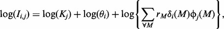where I_i,j denotes the observed intensity for probe i in CEL file j, K_j is the file-specific scaling that accounts for the need for standardization and θ_i represents the extra propensity of probe i (as opposed to an average probe) to stick to a random selection of genetic material. These latter values are chosen so that ∑_∀i log(θ_i) = 0. The term r_M is a motif-specific multiplier that applies to the binding of a probe with material containing the reverse complement of motif M, with δ_i(M) being a multiplier that takes the value 1 if probe i contains motif M, and is otherwise 0, and with ϕ_j(M) being the proportion of genetic material for CEL file j that would bind with the motif M.

The K_j term can be removed by subtracting the mean of the log(I_i,j)-values. It is also convenient to divide by their standard deviation (s.d.) since this gives standardized values {S_i,j} that permit easy comparisons between CEL files, between experiments and between platforms.

Consider a particular five-base motif, M₀, say, which typically occurs in tens of thousands of probes. Rewrite the relation as:

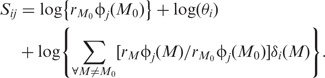We now average over all probes containing M₀. Each probe will have a different relation, but all will have the same first term and the average of the remaining terms will be near zero. An approximation for the average, , is therefore

A minority of the probes containing M₀ will correspond to expressed genes. However, because the average is being taken over so many probes, it is reasonable to assume that both the overall contribution from those genes and the contribution from the log{ϕ_j(M₀)} term can be jointly represented by the sum of a constant, μ, and an error, ϵ, giving the simple linear model

In this formulation, each five-base motif would have its own parameter, λ_M; but, in what follows, we write the 1024 individual parameters as linear combinations of a much smaller number of parameters that describe the base sequences in the various motifs, and thereby provide insights into the factors influencing probe values. More details of the model are given in the Supplementary Material.

In a recent article, McCall et al. (21) examined 24 381 CEL files from 809 GSEs. They judged 2353 (∼10%) to be of low quality. However, these ‘low-quality’ files were not randomly distributed amongs the GSEs: 550 GSEs (containing 11 375 CEL files) were given a clean bill of health, whereas there were 48 GSEs in which every file (a total of 732 CEL files) were judged to be of low quality.

Given that some experiments were found to consist entirely of low-quality arrays, it is not surprising that McCall et al. concluded that ‘some labs are more likely to provide poor quality arrays than others’. However, they cautiously noted that ‘it is conceivable that a study using a non-standard hybridization protocol or investigating a particularly unusual tissue type might appear to have poor quality,’ and concluded that ‘Nevertheless, combining these arrays with arrays from any other experiment would certainly not be advisable.’

In the current article, we report the results of a similar wide-scale screening of CEL files covering Affymetrix platforms for various tissue types. Our results throw some light on the ‘low-quality’ arrays. We have found that the probe values in these arrays are not randomly different from those anticipated, but simply follow a different set of ‘rules’. We also find that it is batches (groups of files processed on the same day) that vary, rather than laboratories.

MATERIALS AND METHODS

The data analysed

Rather than working with the standardized values of individual probes, we work with the average standardized values of groups of probes, with, typically, 25 000 probes in a group. With such large numbers of probes being averaged, it is reasonable to assume that the biological variations (θ_i,j) will effectively average to zero. If the probes had nothing in common then the ϕ_i-values would also be eliminated, but this does not occur since the groups are defined by the common characteristic that every probe in a group contains the same five-base sequence (this choice is discussed in the next section). Since each base is either a C, A, G or T, it follows that there are 4⁵ = 1024 possible groups. Our aim is to identify the causes of variation in these 1024 group averages. The variation in these averages is considerable (typically two SDs, which is of the order of 100 times that expected by chance). We will show that, on average, 86% of this variation can be accounted for using a model with just 22 explanatory variables, while the addition of a further 22 variables results in an explanation of better than 90% of the variation for almost every CEL file.

Both PM and mismatch probes are included in the group selections. Since a 25-base probe contains 21 overlapping five-base subsequences, its standardized value therefore usually contributes to 21 group averages. In cases where a five-base subsequence occurs more than once in the 25-base sequence, it is nevertheless included just once in the average corresponding to that subsequence.

We work with five-base sequences rather than longer sequences so that the averages are calculated from good numbers of probes (usually over 1000) when we subsequently examine the effect of location of the sequence within a 25-base probe. If we used longer sequences, then location-specific results would be affected by biological variations.

Selection of CEL files

Our initial results are all concerned with modelling variation in the average values of the 1024 motif-based groups in a set of 10 000 HGU133Plus2 CEL files that were downloaded from GEO (9). The 333 experiments to which that data refer took place between late 2003 and early 2008. Our later results involve examination of some 18 000 other CEL files from nine different Affymetrix platforms. The files analysed were those available in GEO at the times of the various downloads: they were chosen without reference to the purpose of the original biological experiments.

The extent of the variation in the group averages

Given that a group is defined solely by its members having a particular five-base sequence, with no restrictions on the remaining 20 bases, it might have been anticipated that all the averages would be close to the zero overall mean. That this is not the case is demonstrated in Table 1 which shows the motifs associated with extreme values for the 10 000 HGU133Plus2 CEL files.

Table 1.

Entries are the most extreme group averages calculated from the results for 10 000 HGU133Plus2 CEL files

The largest group averages		The smallest group averages
CCCCC 1.05	CCGCC 1.04	AATTT−0.30	AATTA−0.28
CCTCC 0.97	CTCCC 0.88	ATTTA−0.28	TAATT−0.28

The units are SDs of the standardized probe values.

Table 1 shows that probes containing five-base sequences that include many cytosines are likely to have much greater values than the average probe. However, we show later that this enhancement is largely due to the base sequences concerned rather than the number of cytosines that they contain. Note the contrast between the absolute magnitudes of the largest values and of the smallest values in Table 1. The latter are much smaller and are most likely a consequence of the monomers and dimers forming these five-base sequences since most influential motif-related effects are found to have large positive values (Table 3).

Table 3.

Entries are the mean parameter estimates for the 26 dummy variables forming part of a multiple regression model fitted to each of 28 000 CEL files over 10 platforms (see the Supplementary Material for the results for the seven other platforms)

	Human HGU133+2	Mouse MOE430A	Arabidopsis ATH1-12501
CCCCC	0.55	0.56	0.32
CCCGCCCC	0.40	0.34	0.37
CCGCCTCCC	0.46	0.42	0.34
TCGCCGCT	0.25	0.28	0.27
CCCCG	0.26	0.19	0.29
GGGG	0.33	0.37	−0.03
(AT)CCGC	0.24	0.23	0.21
GCCCG	0.10	0.17	0.19
AGGCCA	−0.20	−0.18	−0.17
CCCCTC	0.28	0.21	0.10
CTGCCT	0.19	0.20	0.12
CTGGCC	−0.16	−0.15	−0.18
AACCC	−0.16	−0.19	−0.09
TCGCTC	0.12	0.13	0.19
GGGGG	0.13	0.14	−0.04
ACGCCA	0.14	0.14	0.16
NotAorT	−0.14	−0.12	−0.17
TCCCC	0.20	0.12	0.10
TCCCT	0.20	0.20	0.07
TGGGG	−0.15	−0.11	−0.12
GCTCCTCG	0.13	0.14	0.11
GGTTGCCC	0.08	0.09	0.10
GAACCA	−0.13	−0.12	−0.09
GGTGCT	0.04	0.07	0.18
GCCCTCCG	0.11	0.12	0.06
GTGGTTC	0.06	0.07	0.15
Median R2	91%	91%	86%
No. of files	10 000	1556	2288
No. of GSEs	322	107	160

The units are SD of logarithms of the raw data. Values of 0.25 SD or greater are shown in bold.

However, when we ask, for each CEL file, which average is largest and which is smallest, we obtain some surprising results, as Table 2 demonstrates. The two motifs GGGGG and TTTTT are highlighted because they feature in both parts of the table. Generally, GGGGG probes have higher than average probe values and on 8% of occasions they have the highest average of all 1024 groups. Nevertheless, there were four files where the GGGGG mean was the lowest of all. Conversely, the mean for TTTTT probes was the lowest on 2% of occasions, but nevertheless there were 11 files for which it had the highest mean. Note that only a minority (60) of the 1024 base sequences feature in the table. The message conveyed by Table 1 was that there are considerable motif-related differences in probe values. The message from Table 2 is that there can be huge variations in the importance of the various motifs from one CEL file to another. It is the nature of these effects and their variations that we seek to uncover in what follows.

Table 2.

Frequencies with which selected group averages were the largest or smallest within their CEL file

Largest	CCCCC	CCGCC	CCTCC	GGGGG	CTCCC
No. of files	3859	3451	1432	832	160
	GGCGG	4 others	TTTTT	9 others
	132	100	11	23
Smallest	AATTT	GCGCG	AATTA	TTTTA	CGCGA
No. of files	6023	1240	808	546	419
	TTTTT	ATATA	34 others	GGGGG
	181	151	632	4

A total of 10 000 HGU133Plus2 CEL files were examined.

Strategy for variable selection

Since the base sequence of a probe affects its expression level, we begin with a three-parameter model (described below) that takes account of the frequencies of the four bases in a 25-base probe. A second model adds a further 15 parameters to take account of the frequencies of the 16 possible dimers. We next add a dummy variable that takes the value 1 if a probe contains a GGGG sequence and otherwise takes the value 0. This model explains 80% of the observed variation.

These first models take account of effects already known to be relevant, whereas each subsequent model is determined from an examination of the residuals of the previous model. Each model is separately fitted to thousands of CEL files and, in each case, we determine the locations of the largest residuals. If a particular motif-based group is persistently associated with a large residual, then this indicates a need for a new dummy variable to take account of that group. In practice, it is not necessary to have a separate dummy variable for every outlier, since we find that many outliers have similar-sized residuals, so that all can be compensated for by using a single dummy variable.

Position-independent models using only quantitative variables

Obviously most 25-base probes will contain at least one example of each type of base; however, our groups of probes are defined by the five-base motif that they are known to contain, and, since we are working with averages over ∼20 000 probes, we can reasonably argue that the average composition of the remaining 20 bases will be approximately the same in each case. Model 1 therefore considers only ‘the numbers of the various bases that occur in the five-base motif that defines the group’ and it ignores the position of the group within the 25-mer.

where is the motif average, x_A, x_C and x_G are, respectively, the numbers of adenines, cytosines and guanines in the motif, ϵ is the error term and β_A, β_C and β_G are the parameters of interest. There is no need to include an x_T term since its value is determined by the fact that x_A + x_C + x_G + x_T = 5 so that, for example, β_A measures the effect on the motif average of that motif including an adenine as opposed to a thymine. For this model, and for all subsequent models, we used as weights to be applied to the 1024 data items, the numbers of probes that were averaged to obtain those data items. Model 1 has just four parameters, but nevertheless explains 50% of the variation in the 1024 motif averages (R² = 50%). Cytosines are known to be linked to larger probe values and adenines to smaller values (22). Note that, at this stage, we are ignoring the within-probe position of the bases; position is relevant (22) but variation with position is a relatively minor affair compared with the motif-based effects observed later.

Dinucleotides also have a bearing on probe values (23); a natural extension of Model 1 is therefore

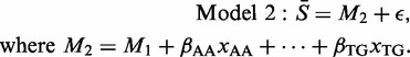This model adds a further 15 parameters to model M₁, with, for example, β_AA measuring the effect on a motif average of that motif including the dinucleotide AA, as opposed to TT. For a dinucleotide involving different bases (e.g. AC), the possible x-values are 0, 1 and 2. For a dinucleotide involving a repeated base (e.g. AA), the values range from 0 to 4. On average, this 19-parameter model explains 78% of the variation in the 1024 data values for a single CEL file.

It should be noted that it is the ‘structure’ of these models that is constant across CEL files, ‘not’ the parameter estimates. We examine the variation in the estimated parameter values later.

Outliers and the identification of relevant dummy variables

Probes that contain the GGGG sequence have values that may be affected by the formation of G-quadruplexes (18) with the consequence of misleading probe values (14). It can scarcely be a coincidence that the more recent Affymetrix platforms have relatively few such probes. A relevant model is therefore

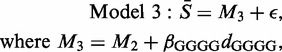where d_GGGG takes the value 1 for the seven groups (GGGGG, CGGGG, AGGGG, TGGGG, GGGGC GGGGA, and GGGGT) containing the GGGG sequence, and otherwise takes the value 0.

In the context of an analysis of variance table, the significance of the extra parameter is beyond doubt, since this model results in an increase of R² from 78 to 80% at the expense of a single extra parameter. Nevertheless, 20% of the variation in the 1024 mean values remains unexplained. In order to see where the model is ineffective, we examined the model residuals (the differences between the observed and fitted values) recording, for each CEL file, the motifs associated with the five most extreme residuals. With 10 000 CEL files and 1024 candidate motifs, if there were no consistent pattern, then each motif would be selected about 50 times. In practice, a few motifs were consistently selected. These dominant motifs (all under-estimated), and the proportion of times on which they were identified, were CCGCC 94%; CGCCT 90%; CCTCC 91%; CTCCC 82% and GCCTC 66%. Notice that three of these appeared in Table 1 (the others were also in the top 10 group means). Other motifs appeared far less frequently and, since those identified are the five subsequences of CCGCCTCCC, and the estimated residuals were similar in magnitude, the next model studied was

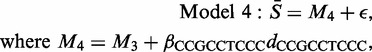where d_CCGCCTCCC takes the value 1 for the five groups (CCGCC, CGCCT, GCCTC, CCTCC and CTCCC) and otherwise takes the value 0. On average, Model 4 explained 85% of the variation in the motif averages. The comparison with Model 3 implies that this single dummy variable has explained 5% of the variation and is therefore of the utmost importance.

In order to verify that it was reasonable to assign the same importance to each of the five subsequences, we next examined the goodness of fit of the set of related Models 4a to 4e.

Comparison of the fit of Model 4 with that of each of Models 4a to 4e provides a test (using the F_1,1002-distribution—see the Supplementary Material for details) of the null hypothesis that β_CCGCC = ··· = β_CTCCC(=β_CCGCCTCCC) against the alternative that (for example) β_CTCCC has a different value. The observed proportion of cases in which the F-ratio exceeded 6.66 (the upper 1% point of the F_1,1002-distribution) were as follows: CCGCC 57%; CGCCT 1.7%; GCCTC 9.1%; CCTCC 3.1% and CTCCC 9.6%. Evidently, the CCGCC motif plays a role in other sequences in addition to its role as part of CCGCCTCCC (the same, but to a much lesser extent, applies to CTCCC and GCCTC) so we took Model 4a (=M₄ + β_CCGCCd_CCGCC + ϵ) as our new starting point.

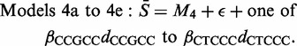
There are again consistent outliers for Model 4a, namely CCCTC 89%; CCCCC 87% and CCCCT 77%. Since these form sections of the longer CCCCCTC motif, the next models considered were

For Model 5, we find a median R²-value of 86%. Since Models 5a to 5c only rarely (see the Supplementary Material for details) provide significant improvements on Model 5, we refer to the single motif CCCCCTC, rather than the separate motifs CCCTC, CCCCC and CCCCT. Model 6 is based on Model 5 and further details of the iterative process of testing and verification are provided in the Supplementary Material. Following this process, the final model contained the 26 dummy variables given in Table 3.

RESULTS

Importance of motifs

The 26 dummy variables that were significant (at the 0.01% level) for at least 10% of the CEL files examined in at least 1 of the 10 platforms considered, are listed in Table 3 in an order that approximates to their overall importance. The estimated values are given in units of SDs, with values of 0.25 sd or above shown in bold type. Results for other platforms are given in the Supplementary Material.

In Table 3, any five-base parameter applies to a single group mean, any six-base parameter applies to two groups, any seven-base parameter applies to three groups and so forth. The (AT)CCGC parameter applies to the two groups ACCGC and TCCGC. The ‘NotAorT’ parameter applies to the 32 groups whose definitions contain neither an A nor a T, while the GGGG parameter refers to the seven groups containing the GGGG sequence in their definition. In each case, the accompanying dummy variable takes the value 1 for any group to which the parameter applies and otherwise takes the value 0.

Although the results given here emanate from a model with 26 dummy parameters, it does not imply that all these parameters are needed for any one CEL file. Although parameters near the top of Table 3 provide a highly significant contribution to the model fit for nearly every CEL file, those near the bottom are required only for subsets of the data. A reduced model, with a dozen parameters would generally be nearly as effective—but it would not be the same reduced model in every case.

Motifs rich in Cs and Gs

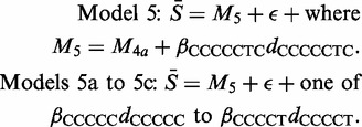
Table 3 is dominated by motifs rich in Cs and Gs. For 7 of the 10 platforms, the largest parameter estimate is β_CCCCC. The second largest is the β_CCCGCCCC parameter relating to the four groups defined by the CCCGC, CCGCC, CGCCC and GCCCC motifs. In addition to the β_GGGG parameter, there are also parameters corresponding only to the CCCCG, GCCCG and GGGGG groups, and the parameter β_NotAorT which relates to the 32 groups (including all those previously mentioned) that are defined without reference to an A or a T. It can be seen that some of these groups that are defined by C/G rich motifs are subject to several dummy variables. Two examples are

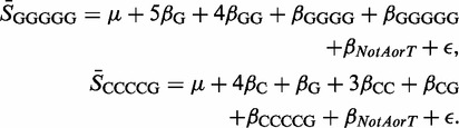It is known that runs of guanines or cytosines influence hybridization behaviour on microarrays so that higher order interaction terms would be needed to improve a model of hybridization intensity (24). Table 4 shows that while the popular HGU133Plus2 and HGU133A arrays contain large numbers of both poly-G and poly-C probes, Affymetrix has designed their more recent platforms with a probe choice that avoids long sequences of Cs and Gs and, in particular, avoids probes containing GGGG sequences. The latter is doubtless because such probes are liable to form G-stacks, structures resembling G-quadruplexes (18).

Table 4.

The numbers of probes (PM and mismatch) containing G/C-rich motifs, together with the median and maximum frequencies of occurrence of the 1024 five-base motifs for 10 Affymetrix platforms

Platform	5Gs	Other GGGG	5Cs	Average G/C rich	All 5-base motifs
					median	max
U133+2	13 000	20 000	8600	10 000	24 000	64 000
U133A/A2	7000	10 000	4300	5000	10 000	25 000
ATH1	1800	4400	1100	4500	10 000	32 000
DrosG	830	2500	1100	7900	7900	22 000
Rice	240	520	700	17 000	26 000	61 000
Mouse4302	200	440	940	5900	20 000	53 000
Barley1	190	1500	900	6100	9400	28 000
Soybean	170	420	820	7100	20 000	60 000
Dros2	2	41	93	7700	11 000	24 000

Entries are correct to two significant figures.

We have argued elsewhere (14,18) that poly-G probes should be excluded from calculations of gene expression because of their propensity to form G-stacks. Despite the near-zero estimate for the Arabidopsis platform (Table 3), Table 5 suggests that poly-G probes should be excluded for this platform also. In the table, the entries are average correlations (×100) between members of two probe sets (self-correlations are excluded). The probe sets were randomly chosen from among those with an ‘at’ extension that were known to contain exactly one probe with a GGGGG sequence. The probe values have been standardized as described previously and it can be seen that the GGGGG probes are more highly correlated with each other (r = 0.74) than they are with the other members of their own probe set (average r-values of 0.18 and 0.21).

Table 5.

Average cross-correlation (×100) of selected probes in unrelated probe sets

	245767_at		246043_at
	GGGGG probe	Other probes	GGGGG probe	Other probes
245767_at
GGGGG probe	NA	18	74	6
Other probes	18	30	8	−4
246043_at
GGGGG probe	74	8	NA	21
Other probes	6	−4	21	25

Probes containing GGGGG and the ATH1-12501 platform.

We detected the problem caused by poly-G probes through an examination of correlations of probes both within and across probe sets. Table 6 shows that similar results occur for probes containing runs of five cytosines.

Table 6.

Average cross-correlation (×100) of selected probes in unrelated probe sets

	1556038_at		1556502_at
	CCCCC probe	Other probes	CCCCC probe	Other probes
1556038_at
CCCCC probe	NA	−12	61	−5
Other probes	−12	11	−9	6
1556502_at
CCCCC probe	61	−9	NA	−4
Other probes	−5	6	−4	9

Probes containing CCCCC and the HGU133Plus2 platform.

CCGCCTCCC and the T7 primer

The high cross-correlations observed in Tables 5 and 6 reflect the chip-to-chip variations in the (generally large) magnitudes of the estimated dummy parameters; similar large cross-correlations are to be expected for probes containing sections of ‘any’ of the motifs near the top of Table 3. One such is the CCGCCTCCC sequence which is the complementary motif to the leader sequence (GGGAGGCGG) of the T7 primer used by Affymetrix (19). Because of the length of this sequence, many probes are potentially affected. Table 1 of (19) gives the numbers of PM probes affected, but it understates the case because it does not consider all possible subsequences (e.g. it considers probes containing CGCCTCCC, but not those containing CCGCCTCC). Mismatch probes will also be affected and, depending on the processing method, these may also impact upon the estimate of a gene's expression. Table 7 gives the relevant frequencies for the HGU133Plus2 platform which contains 604 258 PM probes. More than one-third of the PM probes are liable to have their values inflated as a consequence of having a subsequence of four or more bases in common with the CCGCCTCCC motif.

Table 7.

Frequencies (for the HGU133Plus2 platform) of PM probes, mismatch probes (MM) and PM–MM pairs that contain subsequences of the CCGCCTCCC motif

Subsequence length	9	8	7	6	5	4
PM only	0	7	141	1187	6574	24 762
Mismatch only	1	15	186	1164	6536	20 247
Both	4	55	768	6024	36 336	184 639
Total	5	77	1095	8375	49 446	229 649

We have noted that probes containing subsequences of an influential motif will be correlated. Table 8 shows that the problem is not confined to five-base sequences, but is more widespread. The table shows the correlations between Probe 4 of the 1552808_at probe set (which includes the CCGCCTC sequence in its definition) and members of the otherwise unrelated 1552884_at probe set. Each of the Probes 1–8 in the latter probe set contain at least one four-base subsequence of CCGCCTCCC, whereas Probes 9–11 do not. The results demonstrate that probes that contain extended subsequences of CCGCCTCCC resemble each other much better than they resemble other members of their own probe set (which are strongly correlated with each other). These probe sets were chosen arbitrarily on the basis of the probe compositions and we believe that the pattern of correlations displayed will be typical of other such pairs.

Table 8.

Average cross-correlation (×100) of selected probes in unrelated probe sets

	1552808_at		1552884_at
	CCGCCTC probe	Other probe	Probes 1–8	Probes 9–11
1552808_at
CCGCCTC probe	NA	−10	26	−10
Other probes	−10	13	−13	4
1552884_at
Probes 1–8	26	−13	33	10
Probes 9–11	−10	4	10	52

Probes containing subsets of CCGCCTCCC and the HGU133Plus2 platform.

Five groups of motifs

Although Table 3 lists 26 separate motifs, we do not believe that these are 26 separate effects. Studying the parameter estimates for each platform, it is apparent that there are strong correlations between the estimates for certain pairs of motifs. For example the correlation between the estimates for CCCCTC and TCCCC is 0.89, clearly reflecting their basal similarity. Being guided by these most extreme correlations, we can subdivide the motifs into five groups. Group A consists of CCCCC and four closely related motifs, while Group B consists of CCGCCTCCC and 10 others. These account for the majority of cases where probe values are increased. Group C consists of the six motifs with model parameters having consistently negative values. Group D refers to the G-quadruplex motifs, while Group E refers to two motifs whose estimates are negatively correlated with Group D. Table 9 reports the average correlations (based on results from 10 platforms with over 28 000 files) for the members of these five groups.

Table 9.

Correlations between five groups of motif estimates (based on results for 28 000 CEL files)

	A	B	C	D	E
A	0.48	0.29	−0.34	0.12	0.09
B	0.29	0.60	−0.42	0.25	−0.29
C	−0.34	−0.42	0.41	−0.24	0.17
D	0.12	0.25	−0.24	0.32	−0.41
E	0.09	−0.29	0.17	−0.41	0.80

Group A: (CCCCC, CCCCTC, CCCCG, TCCCC, TCCCT); Group B: (CCGCCTCCC, CCCGCCCC, TCGCCGCT, (AT)CCGC, CTGCCT, ACGCCA, TCGCTC, GCTCCTCG, GCCCTCCG, GGTTGCCC, GCCCG); Group C: (AGGCCA, CTGGCC, TGGGG, NotAorT, GAACCA, AACCC); Group D: (GGGG, GGGGG); Group E: (GGTGCT, GTGGTTC). Correlations with magnitudes in excess of 0.4 are in bold.

There are strong within-group correlations for all groups except group D where the GGGG and GGGGG dummy variables can (to an extent) substitute for one another. With the exception of the two negative correlations, the remaining correlations are comparatively small, suggesting that there are (at least) three ‘separate’ positive effects present (represented by Groups A, B and D). The negative correlations between Group C and Groups A and B (and D) are not induced by the process of fitting the model, so we ascribe them to the standardizing of each CEL file to have mean 0: thus it appears that probes containing these basal strings are particularly unlikely to have values inflated by non-specific binding. We discuss Group E in the next section.

Variation with experiment (GSE)

Figure 1 presents scatter diagrams of estimates of β_CCCGCCCC and β_AGGCCA against time for the HGU133Plus2 data. All data from a single experiment that were processed on the same day have been summed, so as to reduce the 10 000 CEL files to 1523 day-GSE combinations. One group (circles) has near-zero estimates for each motif. Calculations (not reported in this article) suggest that the probes in this group are subject to unusually high degradation. A second group (crosses) have typical values for β_CCCGCCCC (albeit possibly declining over time), but very low values for β_AGGCCA. The definitions of the two groups are given in Table 1 of the Supplementary Material.

Figure 1.

Scatter diagrams showing estimates (values are SD and result from the final model being applied to the pooled data for each of 1523 day-GSE combinations for the 10 000 CEL files relating to the HGU133Plus2 platform) for the CCCGCCCC and AGGCCA parameters plotted against date of scan. In each case, there is one large group plus one or two well-defined smaller groups. One group (circles) take near zero values for each parameter. The second group (crosses) behaves normally with respect to CCCGCCCC but has very low values for AGGCCA.

As for the GNUSE study (21), it is apparent that only a minority of experiments display highly atypical results, though the consistency of these results leads us to conclude that it would be incorrect to label them as being of ‘poor quality’—their quality ‘may’ be as high as the remainder, but the values of the group means are governed by different ‘laws’. Table 2 of the Supplementary Material gives, for each platform, details of experiments (GSEs) for which the parameter estimates are unusual when compared with the bulk of the GSEs examined for that platform.

The variation between experiments is particularly apparent in the context of Group E of Table 9. For most platforms, the parameter estimates for the two motifs in this group have modest values. The principal exception is for the Arabidopsis platform. There, closer inspection reveals that the largest values arise predominantly from just a few experiments. In particular, nine GSEs (248 CEL files) that result from the participation of researchers at five German universities in the AtGenExpress initiative account for 227 of the 572 in the upper quartile of the estimates for GTGGT. The cause is not known but it may be related to the German team's deliberate choice of a low amount of input RNA (2 μg max.) prior to labelling and amplification (Dierk Wanke, Personal communication; see also (25) for related information). It is possible that some alternative quadruplexes involving thymines as well as guanines are being formed.

Variation between batches

Figure 2 shows scatter diagrams for β_CCGCCTCCC for three GSEs chosen because their results were obtained over a period of >18 months using a single scanner throughout. The areas of the plotting symbols are proportional to the numbers of CEL files processed on that day: the plot for GSE7307 presents information for 56 days, with an average of 12 CEL files per day, with the corresponding figures for GSE8052 and GSE 9891 being (61; 7) and (56; 5), respectively. Figure 1 showed that there were clear distinctions ‘between’ GSEs; Figure 2 shows that there are also important variations ‘within’ GSEs. Although the earliest results for GSE7307 and the latest results for GSE9891 demonstrate short-term consistency, neither group is typical of the remainder for that GSE. The values for GSE7307 appear to slowly decline suggesting the possibility of long-term trends, while the plots for both GSE7307 and GSE8052 show extreme outliers that are based on the averages of good numbers of individual CEL files.

Figure 2.

Scatter diagrams showing, for three individual GSEs, estimates (values are s.d.) for the CCGCCTCCC parameter against time of scan. Each plot shows the average value of the estimates for a batch (CEL files scanned on the same day), with the areas of a circle being proportional to batch size.

Variation within a batch

Averages can be misleading, so we now examine the variation observed from one CEL file to another within a single day's activity.

Table 10 shows the estimates for the β_CCGCCTCCC parameter for 2 days of processing for the GSE7307 experiment. Average daily values for this experiment were plotted in Figure 2. The first set, taken from late on New Year's Eve 2003, nevertheless shows entirely typical values for the parameter (unaffected by festivities!). By contrast, the second set of observations (corresponding to the outlier in Figure 2) contain a sprinkling of extreme outliers, with only one of the 17 values being lower than the mean of the previous group. The same scanner was used for all the CEL files.

Table 10.

Examples of variations in parameter estimates within a single day

GSM	GSE7307 CEL files on 31 December 2003 (19:00 to 23:45)
175786-92	0.28		0.36	|	0.26		0.26		0.30		0.26		0.28
175793-4, 7-801	0.42	|	0.24		0.25		0.30		0.26		0.37		0.45
175802-3, 5-6, 9	0.29		0.44		0.36		0.52		0.54

GSM	GSE7307 CEL files on 4 November 2005 (11:00 to 15:00)
176301-07	0.48	|	1.63		1.11	|	0.51		1.75		0.44	|	1.47
176308-14	0.39		0.98		0.48		1.26		1.45	|	0.42		0.34
176315-17	1.42		1.25		0.33

The values are the estimates for the β_CCGCCTCCC parameter. The values are given correct to two decimal places and are presented in the order of the scans. The scans were consecutive except where indicated with a ‘|’ symbol.

Carousels

To confirm that biases were not related to carousels (which can result in a sequence of 48 arrays being scanned without operator intervention) we show, in Table 11, the estimates for the β_CCGCCTCCC parameter during an uninterrupted 4-h period where each CEL file was processed within 11 min of its predecessor. The file identifiers are given in the table in order to emphasize that CEL files may not be processed in numerical order. However, a study of the autocorrelation between successive estimates based either on their numbering, or the order of processing, show near-zero values at all lags.

Table 11.

Example of the parameter estimates resulting from a single carousel run

File id	507	510	516	518	519	520	443	549
Estimate	0.62	0.63	0.64	0.72	0.62	0.67	0.84	0.66
File id	466	467	468	497	498	499	500	501
Estimate	0.49	0.61	0.66	0.57	0.61	0.66	0.54	0.53
File id	502	524	530	488	490	491
Estimate	0.53	0.48	0.50	0.57	0.50	0.63

The scanner id was 50201191. The first file was timed at 10:03:37 on the 2nd March 2006 and the last file at 13:59:59 on that day. All the experiments form part of GSE2109. The ids given should be preceded by GSM102 (so that 507 refers to GSM102507).

Conclusions concerning batch variation

Figure 2 hints at short-term consistency in terms of averaged parameter values. By contrast, Tables 10 and 11 demonstrate that, even on a good day, parameter estimates can vary by a factor of 2 between one CEL file and another. Some of that variation is undoubtedly due to the uncertainties inherent in the multiple regression process, but some must surely be genuine. The apparent absence of trends within a day's processing suggests that, in general, the variation occurs at the time that the microarray is processed, and not at the time at which it is scanned. An exception, where it is the scanner that is causing problems, is where the scanner reports a blurred image (13).

Variation with probe segment

It is well known (22,23) that the effects of the alternative nucleotides and dinucleotides vary with location within a 25-mer probe (being least pronounced at either end of a probe). We have therefore examined the effect of location on the motif-related biases that we have uncovered. Since there are 21 possible locations for a 5-mer subset in a probe, the numbers of probes over which we take averages is occasionally just a few hundred (though it is typically over a thousand). Results here are therefore more likely than the previous results to be influenced by biological variations.

Figure 3 shows the impact of position on the parameter estimate (the probe's free end is base 1). For clarity, the data have been smoothed using Friedman's variable span smoother (26). We have confined attention to the six most important motifs, and the results reported are for a random sample of 2000 HGU133Plus2 CEL files.

Figure 3.

Changes in the estimates of the dominant parameters according to the location of the 5-mer section within the 25mer probe. The individual values have been smoothed using Friedman's variable scan smoother.

For most motifs, there is a reduced effect near the tethered end of the probe, with interesting variations at the untethered ends. In most cases, there is a decreased effect at the untethered end which may be attributable to the efficiency of the lithographic process being less than perfect (so that not all the individual strands have a full 25-base length). The striking exception is that the impact of G-quadruplexes is at its greatest when the GGGG sequence is near the free end of a probe, presumably because the greater flexibility at this untethered end makes it easier for G-quadruplexes to form.

Fasold et al. (20) have suggested that the formation of G-quadruplexes might be facilitated by the presence of high levels of the T7-primer, with this being most marked at the free end of the probes. Table 9 did indeed shows a modest positive correlation between the relevant motif groups. However, when attention is confined to bases 1–5, and to the estimates corresponding to CCGCCTCCC and GGGG alone (rather than using groups), the correlation (based on the 10 000 HGU133Plus2 CEL files) is near zero (−0.06). This supports our view (14,18) that the effects are not linked. We suggest that variations in the magnitude of the GGGG estimates reflect variations in contaminants associated with the hybridization protocol, such as the concentration of K+ or ethanol (18).

The design of Affymetrix microarrays recognizes that the central base is the most sensitive to the presence of a target gene (because binding with the target is more likely to result in an overlap with that base, than with any other). Since a probe can only bind once, then, if it is binding to its target, it is not binding to an unwanted motif fragment. We believe that this explains the tendency for the motif-related effects to show slight reductions near the central bases.

The extent of motif bias

Table 3 gives an idea of the ‘magnitude’ of the motif-related biases, and Table 7 gives an idea of the frequency of occurrence for a single motif. However, there are many motifs involved, so there are many possible ways in which a probe may be affected. Table 12 provides more detailed information for the HGU133Plus2 array.

Table 12.

The numbers (and percentages) of PM probes, on the HGU133Plus2 array, that have five-base (or longer) probe sequences in common with the most influential motifs

CCGCCTCCC	GGGG	CCCCTC	CCCGCCCC
51 545 (8.5%)	32 538 (5.4%)	23 694 (3.9%)	18 667 (3.1%)
TCGCCGCT	CCCCC	CCCCG	None of these
14 319 (2.4%)	4255 (0.7%)	3369 (0.6%)	494 561 (81.8%)

Each of the seven motifs included in Table 4 results in an average increase in a probe value of at least 0.25 sd. The HGU133Plus2 platform contains 604 258 PM probes implying that nearly 20% are likely to be affected by at least one of the seven selected motifs. There will be many other probes that are affected by at least one of the less influential motifs.

Probe sets typically include 11 probes, so a probe set will be unaffected only if none of its members are affected. Restricting attention only to the seven most important motifs, we find that ∼80% of probe sets contain at least one affected probe, while about one-third of probe sets have at least three affected probes. Of course, since procedures such as GCRMA use information from neighbouring probes, it is likely that ‘all’ expression measures will be affected to some extent.

Impact on the estimates of parameters relating to mononucleotides and dinucleotides

It is known that cytosines are linked with higher probe values (23). Table 3 is dominated by motifs that are rich in cytosines, so there is the possibility that the cytosine-related higher probe values are an artifact induced by the motifs. Table 13 demonstrates that this is not the case, since the model that contains only dummy parameters does not provide an adequate fit to the data: both sets of quantitative parameters are required. Further improvements (though with many more parameters) would result from including position dependence as suggested by Figure 3.

Table 13.

Median R²-values for selected models fitted to 10 000 CEL files using the HGU133Plus2 platform

Dummy parameters only	41%	Mononcleotides only	50%
Mono- and dinucleotides only	78%	Full model	91%

DISCUSSION

Microarrays are, and have been for the last decade, a pervasive technology in the life sciences. There are now >10⁵ Affymetrix GeneChips in GEO that have been deposited following papers and contributions from thousands of scientists. GeneChip technology, and its protocols, are probably the best example of ‘factory’ science that we have in the 'omics field. Due to this widespread use and standardisation, and due to of the public availability of the data, GeneChips appear to provide a unique opportunity to develop meta-analysis of the behaviour of individual probes across multiple experiments, and to compare the behaviour of multiple probes across individual experiments. However, the results presented in this article present a sharp warning to would-be meta-analysts, since they reveal considerable non-biological variations between CEL files batches of CEL files and whole experiments.

We are confident that the motif-finding approach outline here is effective since it has independently picked out effects already known to exist (namely those relating to G-quadruplexes, the T7-primer and high GC content). The additional information provided by our analysis concerns the relative magnitudes of the effects (Table 3), and the extent to which those magnitudes vary both across and within experiments. Models (such as those of (7,22,23)) that do not take account of the magnitudes of these biases will inevitably be over-estimating the effects of the shorter motifs that they consider. In particular, we note the upward bias for β_CC that would result if the effects of β_CCCCC and β_CCGCCTCCC were overlooked.

We suspect that not only the magnitude of the effects but also their extent in terms of numbers of probes affected may not be widely appreciated. Table 7 gave an indication of the numbers for one motif and one platform, with Table 12 providing details for other motifs.

It seems probable that these effects will also hold true for other platforms (such as the increasingly popular RNA-Seq experiments). The presence of motif effects will complicate efforts to obtain reliable estimates of differential expression from any platform. If meta-analyses are to be attempted, then the data must first be purged of the non-biological variations that this article has revealed.

CONCLUSION

Current methods (1,2) for summarizing probe intensities into measures of gene intensity take account of probe composition with respect to monomers and dimers, but take no account of longer motifs. However, in this article, we have demonstrated that there are considerable alterations to probe values that result from the probe composition including segments from one or more influential motifs. These motifs appear to affect all types of GeneChip. For the most used type (the Human HGU133Plus2 platform) nearly 80% of probe sets include at least one affected probe.

The effects of the influential motifs can cause massive distortions to individual probe values, as indicated by Table 3. Figure 2 indicates that the influence varies greatly from batch to batch. The implication is that when one considers probes that share a related motif one is likely to find highly correlated values. With probe sets containing overlapping probes that share an influential motif, the correlation will be particularly high; this may give the observer a false sense that the probe set is measuring variations in the gene for which it was designed, whereas in fact the variation is (at least in part) due to the motif. Similarly, if we study two such probe sets then we might incorrectly conclude that there were relations between the genes concerned when in fact it was the motif that was engendering the association.

What should be done? We suggest that the pragmatic solution is to estimate the sizes of the motif effects and then to adjust all probe values to take account of the motif biases. In practice, this will generally result in a set of reduced values. The revised values can then be analysed using whichever method (e.g. GCRMA) that the experimenters prefer. In their discussion of the effect on probe expression of GGG-sequences Fasold et al. (20) proposed an equivalent solution.

SUPPLEMENTARY DATA

Supplementary Data are available at NAR Online: Supplementary Material.

FUNDING

Funding for open access charge: University of Essex.

Conflict of interest statement. None declared.

REFERENCES

- 1.Irizarry R, Bolstad B, Collin F, Cope L, Hobbs B, Speed T. Summaries of Affymetrix GeneChip probe level data. Nucleic Acids Res. 2003;31:e15. doi: 10.1093/nar/gng015. [DOI] [PMC free article] [PubMed] [Google Scholar]
- 2.Irizarry R, Wu Z, Jaffee H. Comparison of Affymetrix GeneChip expression measures. Bioinformatics. 2006;22:789. doi: 10.1093/bioinformatics/btk046. [DOI] [PubMed] [Google Scholar]
- 3.Geller S, Gregg J, Hagerman P, Rocke D. Transformation and normalization of oligonucleotide microarray data. Bioinformatics. 2003;19:1817. doi: 10.1093/bioinformatics/btg245. [DOI] [PubMed] [Google Scholar]
- 4.Do J, Choi D. Normalization of microarray data: single-labeled and dual-labeled arrays. Mol. Cells. 2006;22:254–261. [PubMed] [Google Scholar]
- 5.Binder H, Preibisch S. Hook calibration of GeneChip microarrays: theory and algorithm. Alg. Mol. Biol. 2008;3:12. doi: 10.1186/1748-7188-3-12. [DOI] [PMC free article] [PubMed] [Google Scholar]
- 6.Mulders G, Barkema G, Carlon E. Inverse Langmuir method for oligonucleotide microarray analysis. BMC Bioinformatics. 2009;10:64. doi: 10.1186/1471-2105-10-64. [DOI] [PMC free article] [PubMed] [Google Scholar]
- 7.Binder H, Kirsten T, Loeffler M, Stadler P. Sensitivity of microarray oligonucleotide probes: variability and effect of base composition. J. Phys. Chem. B. 2004;108:18003–18014. [Google Scholar]
- 8.Burden C. Understanding the physics of oligonucleotide microarrays: the Affymetrix spike-in data reanalyzed. Phys. Biol. 2008;5:016004. doi: 10.1088/1478-3975/5/1/016004. [DOI] [PubMed] [Google Scholar]
- 9.Barrett T, Troup D, Wilhite S, Ledoux P, Rudnev D, Evangelista C, Kim I, Soboleva A, Tomashevsky M, Edgar R. NCBI GEO: mining tens of millions of expression profiles–database and tools update. Nucleic Acids Res. 2006;35:D760–D765. doi: 10.1093/nar/gkl887. [DOI] [PMC free article] [PubMed] [Google Scholar]
- 10.Upton G, Lloyd J. Oligonucleotide arrays: Information from replication and spatial structure. Bioinformatics. 2005;21:4162–4168. doi: 10.1093/bioinformatics/bti668. [DOI] [PubMed] [Google Scholar]
- 11.Arteaga-Salas J, Zuzan H, Langdon W, Upton G, Harrison A. An overview of image-processing methods for Affymetrix GeneChips. Brief. Bioinformatics. 2007;9:25–33. doi: 10.1093/bib/bbm055. [DOI] [PubMed] [Google Scholar]
- 12.Arteaga-Salas J, Harrison A, Upton G. Reducing spatial flaws in replicate oligonucleotide arrays by using neighbourhood information. Stat. Appl. Genet. Mol. 2008;7:29. doi: 10.2202/1544-6115.1383. [DOI] [PubMed] [Google Scholar]
- 13.Upton G, Harrison A. The detection of blur in Affymetrix GeneChips. Stat. Appl. Genet. Mol. 2010;9 doi: 10.2202/1544-6115.1590. Article 37. [DOI] [PubMed] [Google Scholar]
- 14.Upton G, Langdon W, Harrison A. G-spots cause incorrect expression measurement in Affymetrix microarrays. BMC Genomics. 2008;9:613. doi: 10.1186/1471-2164-9-613. [DOI] [PMC free article] [PubMed] [Google Scholar]
- 15.Memon F, Upton G, Harrison A. A comparative study of the impact of G-stack probes on various Affymetrix GeneChips of Mammalia. J. Nucleic Acids. 2010;2010:489736. doi: 10.4061/2010/489736. [DOI] [PMC free article] [PubMed] [Google Scholar]
- 16.Shanahan H, Memon F, Harrison A, Upton G. Normalized Affymetrix expression data are biased by G-quadruplex formation. Nucleic Acids Res. 2012;40:3307–3315. doi: 10.1093/nar/gkr1230. [DOI] [PMC free article] [PubMed] [Google Scholar]
- 17.Memon F, Owen A, Sanchez-Graillet O, Upton G, Harrison A. Identifying the impact of G-Quadruplexes on Affymetrix 3′ Arrays using Cloud Computing. J. Integr. Bioinformatics. 2010;7:111. doi: 10.2390/biecoll-jib-2010-111. [DOI] [PubMed] [Google Scholar]
- 18.Langdon W, Upton G, Harrison A. Probes containing runs of guanines provide insights into the biophysics and Bioinformatics of Affymetrix GeneChips. Brief. Bioinform. 2009;10:259–277. doi: 10.1093/bib/bbp018. [DOI] [PubMed] [Google Scholar]
- 19.Kerkhoven R, Sie D, Nieuwland M, Heimerikx M, De Ronde J, Brugman W, Velds A. The T7-Primer is a source of experimental bias and introduces variability between microarray platforms. PLoS One. 2008;3:e1980. doi: 10.1371/journal.pone.0001980. [DOI] [PMC free article] [PubMed] [Google Scholar]
- 20.Fasold M, Stadler P, Binder H. G-stack modulated probe intensities on expression arrays sequence corrections and signal calibration. BMC Bioinformatics. 2010;11:207. doi: 10.1186/1471-2105-11-207. [DOI] [PMC free article] [PubMed] [Google Scholar]
- 21.McCall M, Murakami P, Lukk M, Huber W, Irizarry R. Assessing Affymetrix GeneChip microarray quality. BMC Bioinformatics. 2011;12:137. doi: 10.1186/1471-2105-12-137. [DOI] [PMC free article] [PubMed] [Google Scholar]
- 22.Naef F, Magnasco M. Solving the riddle of the bright mismatches: labeling and effective binding in oligonucleotide arrays. Phys. Rev. E. 2003 doi: 10.1103/PhysRevE.68.011906. 68, 011906. [DOI] [PubMed] [Google Scholar]
- 23.Gharaibeh R, Fodor A, Gibas C. Background correction using dinucleotide affinities improves the performance of GCRMA. BMC Bioinformatics. 2008;9:452. doi: 10.1186/1471-2105-9-452. [DOI] [PMC free article] [PubMed] [Google Scholar]
- 24.Mei R, Hubbell E, Bekiranov S, Mittmann M, Christians F, Shen M, Lu G, Fang J, Liu W, Ryder T, et al. Probe selection for high-density oligonucleotide arrays. Proc. Natl Acad. Sci. USA. 2003;100:11237–11242. doi: 10.1073/pnas.1534744100. [DOI] [PMC free article] [PubMed] [Google Scholar]
- 25.Wanke D, Kilian J, Supper J, Berendzen K, Zell A, Harter K. The analysis of gene expression and cis-regulatory elements in large mocroarray expression data sets. In: Accardi L, Ohya M, editors. Quantum Bio-Informatics: From Quantum Information to Bio-Informatics. Vol. 21. World Scientific Publishing Co. Pte. Ltd; 2008. pp. 294–314. ISSN: 1793–5121. [Google Scholar]
- 26.Friedman J. Technical Report No. 5. Laboratory for Computational Statistics, Stanford University; 1984. A variable span scatterplot smoother. [Google Scholar]
Associated Data
This section collects any data citations, data availability statements, or supplementary materials included in this article.