3-D Phantom and In Vivo Cardiac Speckle Tracking Using a Matrix Array and Raw Echo Data

Abstract

Cardiac motion has been tracked using various methods, which vary in their invasiveness and dimensionality. One such noninvasive modality for cardiac motion tracking is ultrasound. Three-dimensional ultrasound motion tracking has been demonstrated using detected data at low volume rates. However, the effects of volume rate, kernel size, and data type (raw and detected) have not been sufficiently explored. First comparisons are made within the stated variables for 3-D speckle tracking.

Volumetric data were obtained in a raw, baseband format using a matrix array attached to a high parallel receive beam count scanner. The scanner was used to acquire phantom and human in vivo cardiac volumetric data at 1000-Hz volume rates. Motion was tracked using phase-sensitive normalized cross-correlation. Subsample estimation in the lateral and elevational dimensions used the grid-slopes algorithm.

The effects of frame rate, kernel size, and data type on 3-D tracking are shown. In general, the results show improvement of motion estimates at volume rates up to 200 Hz, above which they become stable. However, peak and pixel hopping continue to decrease at volume rates higher than 200 Hz. The tracking method and data show, qualitatively, good temporal and spatial stability (for independent kernels) at high volume rates.

Introduction

Cardiac tissue motion is potentially the most relevant information for cardiac diagnostics because it represents tissue efficacy [1]. Cardiac motion is used to assess overall function, ischemia, infarct, and arrhythmia. Motion assessment is performed qualitatively and quantitatively, but quantitative methods (for the left ventricle) are more reliable [2]. A notable quantitative metric for cardiac function is the change in wall thickness (strain) between end-diastole and end-systole, which correlates well with cardiac function [3]. Strain is an attractive metric of cardiac function because it is easily measurable by comparing multiple anatomic images provided by imaging modalities such as magnetic resonance (MR) or ultrasound. In principle, the strain between end-diastole and end-systole could be calculated using only 2 images, in practice the rate of strain is usually calculated by estimating the spatial-derivative of velocity estimates. The strain curve through time can be calculated as the temporal integral of the strain rate for a given spatial region [4], [5]. Therefore, strain and strain rate quality are directly related to the ability to measure cardiac tissue velocities.

Cardiac tissues experience a range of velocities during the cardiac cycle. Cardiac velocities have been measured using MR for all 3 dimensions of motion in the cardiac coordinate system by Delfino et al. [6]. They report peak velocities, in humans, of 6.5 ± 2.2, 3.2 ± 1.2, and 12.0 ± 3.1 cm/s in the radial, circumferential, and longitudinal dimensions, respectively. Similar, but slightly lower, velocities have been measured by others [7], [8]. Although the above measurements were cited from MR results, various methods have been developed to capture cardiac motion for both research and clinical purposes.

Ultrasound has been used to measure cardiac dynamics in quantitative and qualitative manners using M-mode and A-mode methods since the late 1940s [9]. In the 1970s, the development of B-mode ultrasound allowed an increased level of qualitative assessment of global and local cardiac motion [9].

Sonomicrometry, developed in the 1970s, uses small piezoelectric crystals embedded in the myocardial surface; the crystals monitor their positions relative to partner crystals embedded at nearby locations. The attached crystal’s time-of-flight data can be reconstructed to acquire estimates of segment dimensions, segment shortening velocities, and metrics of segment power and stroke work [10]. Sonomicrometry provided much of the initial data on cardiac motion and is still regarded as the gold standard for myocardial motion tracking [11].

Myocardial motion has also been tracked by implanting radiopaque beads into the myocardium with known geometry. The beads are imaged at a frame rate of 75 Hz using biplane fluoroscopy [12], [13]. The radiopaque beads’ positions through time can be reconstructed in 3 dimensions to analyze complex myocardial modes, such as rotational dynamics.

Unfortunately, both sonomicrometer and radiopaque bead implantation are highly invasive procedures. Therefore, they have been primarily used to track motion in the canine heart. Although a useful tool for research, these techniques are not practical for clinical cardiac motion diagnostics. Besides lacking clinical practicality, the implantation process causes about 1 mm of scarring around the implanted object [10], which almost certainly alters cardiac motion.

A relatively new technique uses biplane fluoroscopy—but rather than tracking implanted radiopaque beads, it noninvasively tracks distinct features such as coronary arteries [14], [15]. However, this technique has not yet found wide clinical utility.

Another emerging technique is motion tracking with computed tomography (CT). The potential for tomographic velocity estimation has been known for almost 2 decades [16]. The recent commercialization of multidetector and multislice CT scanners may finally result in the realization of CT-based clinical motion analysis [17].

For clinical cardiac motion analysis, there are 2 primary modalities: MR and ultrasound. MR imaging has been used almost since its inception to investigate motion [18], [19]. Motion can be tracked with MR using either phase methods or MR tagging methods [20]. In a general sense, these methods can be compared with ultrasound where MR phase encoding is analogous to ultrasound’s autocorrelation methods, and MR tagging is analogous to ultrasound speckle tracking.

Although MR tracks motion well and has been able to track all 3 dimensions of motion since its inception, MR struggles with poor temporal resolution. The poor temporal resolution of MR has been circumvented by reconstructing 3-D cardiac motion across multiple cardiac cycles. New MR scanners with volume rates as fast as 1 volume per second have been demonstrated [21], but these rates are still too slow to capture all the necessary data within a single heart cycle.

Motion can be tracked with ultrasound using phase changes or the intrinsic tissue texture called speckle. Variations on both of these techniques have been around since the 1980s [22], [23]. The original motion tracking techniques employed on ultrasound data were along the transducer’s axial dimension.

The axial dimension is typically the sole dimension used for clinical velocity and displacement estimates, and these estimates are almost always accomplished with Doppler or autocorrelation methods [23], [24]. Despite the clinical success of autocorrelation methods, they are limited to the axial dimension. As an alternative approach and a way to track in multiple dimensions, the speckle tracking methods originally investigated by Embree and O’Brien were adapted to 2-D displacement tracking by Trahey et al. [25]. From here, many variations of 1-D and 2-D speckle tracking algorithms for motion displacement have been applied to ultrasound imaging. These variations include block matching with a wide variety of objective functions, optical flow methods and mixed methods that combine different tracking techniques [26]–[32]. With the introduction of displacement estimation in 2 spatial dimensions, the motion lateral to the transducer’s point spread function could be estimated. However, there is a well-characterized, jitter-based performance penalty for tracking along nonaxial dimensions due to lower spatial frequency content and lack of lateral and elevational phase information [33]. Fortunately, the spatial and tracking resolution in ultrasound competes well with or outperforms other modalities. Because of this, researchers and clinicians have had widespread success with 2-D ultrasound speckle tracking [1]. Despite the success of 2-D speckle tracking, the inability to track through plane motion means that 2-D speckle tracking remains an incomplete solution.

The solution to through plane motion in displacement tracking and the hope of much of the ultrasound research community is volumetric ultrasound. Volumetric ultrasound has been present within the community for more than 2 decades [34]. Despite 3-D ultrasound’s longstanding presence, it has taken some time for it to become clinically widespread. Advanced ultrasound techniques that use speckle tracking—it has been hypothesized—will be particularly benefited by 3-D speckle tracking and the resulting 3-D motion vector [35], [36].

Because of the importance of 3-D speckle tracking, many researchers have devised schemes to create 3-D radio frequency data sets or have simulated these raw 3-D data sets to study the characteristics of 3-D structures or 3-D tracking techniques.

Some attempts have been made to acquire volumetric data by mechanical translation (or rotation) of 1-D arrays [37]–[39]. Although these techniques show some promise, they invariably suffer from some combination of poor temporal and spatial resolution. Because of this, 3-D speckle tracking in dynamic systems of interest (such as the heart) remains elusive.

Some notable simulations and phantom investigations into 3-D speckle structure have been performed by Bash-ford and von Ramm [40], Meunier [41], Chen et al. [36], and Yu et al. [42]. Yu et al. have shown that, for deformations (in a compressional sense) larger than 2%, detected ultrasonic displacement tracking will yield better results than raw echo tracking methods. Yu et al.’s results indicate that the data type employed so far for 3-D tracking (i.e., detected data), which have all been in the heart, are optimal based on the low frame rates used.

The first group to demonstrate 3-D detected speckle tracking was Morsy and von Ramm [43] and more recently Kuo and von Ramm [44]. With the full scale commercialization of 3-D clinical scanners, the last few years have seen many additional studies employing 3-D speckle tracking on detected echo data [45]–[47]. Although these methods have been successful, they have used detected data, which eliminates one of ultrasound’s greatest strengths: axial phase information.

In this paper, 3-D speckle tracking on raw data is validated with a high parallel receive beam¹ count (64-to-1) clinical scanner [49] using a high channel count matrix array [50]. Specifically, 3-D speckle tracking is validated with phantom studies. The performance and feasibility of speckle tracking with raw data in a dynamic system, the heart, is demonstrated. Comparisons are made among different kernel sizes and volume rates.

Additionally, this work compares the performance of motion tracking using detected and raw B-mode echo data. Although the echo data used in this work were acquired in an in-phase and quadrature (IQ) format, several works have shown that there is little difference in the performance between radio-frequency (RF) and IQ data when proper algorithms are employed [51], [52]. In this paper the label “raw” will refer to data containing phase information (IQ or RF), while the label “detected” will refer to echo magnitude data displayed in B-mode images.

II. Methods

A. Method: Data Acquisition

Ultrasound volumetric, baseband data were acquired using a Siemens SC2000 imaging system and a 4Z1C matrix array (Siemens Healthcare Sector, Ultrasound Business Unit, Mountain View, CA) [49], [50]. The scanner was used to acquire both in vivo 3-D cardiac data and 3-D phantom data. Data sets were acquired with a 2.8-MHz transmit frequency and a 1° azimuthal and elevational receive beam spacing. Data were acquired down to 14 cm. Each data set’s region of interest (ROI) and pulse repetition frequency (PRF) were modified based on the desired task. All data were acquired and then processed offline.

Cardiac data sets were acquired on one of the authors (BB), a healthy 27-year-old male with no known cardiovascular defects. The cardiac data were acquired using parasternal, left ventricle, short-axis views. It was not possible to acquire matched ECG data at the time of data acquisition. All temporal registration of the data with cardiac physiology was accomplished by inspecting M-mode sequences reconstructed offline.

Phantom data sets were acquired in a diffusely scattering, speckle-generating medium. A speckle-generating medium contains a high scatterer density at the level of the resolution cell of the imaging system. As the scatterer density increases, the underlying image statistics converge to well-described first- and second-order moments, producing fully developed speckle [53]. The phantom’s attenuation was 0.5 db/cm/MHz.

B. Method: 3-D Speckle Tracking Using Phase-Sensitive Normalized Cross-Correlation

A graphical depiction of 3-D speckle tracking can be seen in Fig. 1. As discussed in the introduction, many algorithms have been proposed for ultrasound time delay estimation. The time delay estimator implemented for this work was phase-sensitive normalized cross-correlation. Phase-sensitive cross-correlation was originally introduced to ultrasound literature by Wear and Popp [54] and was popularized by O’Donnell et al. [55].

Fig. 1.

This figure demonstrates the process of 3-D speckle tracking. 3-D speckle tracking identifies a 3-D kernel within an initial volume. Within a second volume, at a later time, the closest match to the kernel is identified, and the corresponding location is assumed to represent the displacement. Usually the search is performed inside a subset of the second volume for computational efficiency.

The basic assumption of cross-correlation and similar time delay estimators is that the local speckle pattern—caused by the geometry of scatterers in a given tissue volume—remains constant and only undergoes bulk translation [56]. Using this assumption, it is reasonable to define a signal as the convolution of the system’s point spread function, F(), with a scatterer function, H(). A second signal is similarly defined except a shifted version of the scatter function is used. In ultrasonic imaging, the point spread function is not often stationary. However, over a small region, returned echo signals can be approximated by

$$\begin{array}{l}{s}_n(t,x,y)=H(t-{\tau }_n,x-{\xi }_n,y-{\eta }_n)\otimes F(t,x,y)\\ s_{n+m}(t,x,y)=H(t-{\tau }_{n+m},x-{\xi }_{n+m},y-{\eta }_{n+m})\otimes F(t,x,y)\end{array}$$ (1)

where ⊗ denotes the convolution operator, and t, x, and y indicate time, lateral, and elevational dimensions, respectively. The n and m are the discrete slow time indices. Finally, the delays between the 2 signals’ dimensions can be described by τ_n+m − τ_n, ξ_n+m − ξ_n, and η_n+m − η_n relative to the respective dimension.

Generally, the shorter the temporal duration between a signal s_n and s_n+m, the better the approximation of scatterer bulk motion within a resolution cell.

Based on this representation of 2 signals, the corresponding 3-D normalized cross-correlation function is defined in (2), see next page, and was implemented in Mat-lab (MathWorks, Inc., Natick, MA).

When the normalized cross-correlation function is used as a time-delay estimator, the best time delay is assumed to be the maxima of the function. However, the normalized cross-correlation function shown in (2) is complex (because it operates on baseband data), and the best pixilated time-delay estimate will be indicated by the maximum magnitude of the cross-correlation function, which is

$${\rho }_{n,m}(t,x,y)=\frac{{\displaystyle \sum _{\tau }}{\displaystyle \sum _{\xi }}{\displaystyle \sum _{\eta }}{w}_{\tau ,\xi ,\eta }(s_{n,\tau ,\xi ,\eta }-{\overline{s}}_n)(s_{n+m,\tau +t,\xi +x,\eta +y}^{\ast }-{\overline{s}}_{n+m}^{\ast })}{\sqrt{\sum \sum \sum w_{\tau ,\xi ,\eta }{\mid s_{n,\tau ,\xi ,\eta }-{\overline{s}}_n\mid }^2\sum \sum \sum w_{\tau ,\xi ,\eta }{\mid s_{n+m,\tau +t,\xi +x,\eta +y}-{\overline{s}}_{n+m}\mid }^2}}$$ (2)

$$\rho {(t,x,y)}_{\text{mag}}=\mid \rho (t,x,y)\mid$$ (3)

$$t_{max},x_{max},y_{max}=\underset{t,x,y}{argmax}(\rho {(t,x,y)}_{\text{mag}}).$$ (4)

In the proposed method, interpolation is not performed to increase the number of samples either before or after signal correlation. Because no samples are added, the time-delay estimates are coarse. The coarseness of the estimates in the various dimensions is mitigated in 2 ways. First, the coarseness of axial time-delay estimates is eliminated using the phase-sensitivity of the cross-correlation function. Cross-correlation of complex ultrasound data results in averaging the phase difference over a region specified by the kernel size. The axial estimates may be refined optimally by using the phase at the point of maximum magnitude. This process can be considered a spatial variant of common autocorrelation methods used for axial displacement estimation, which features improved SNR and eliminates phase wrapping. Phase wrapping is eliminated by using the gross axial displacement from the maxima of the cross-correlation function to determine how far the tissue has displaced in excess of the ±π displacement limit.

Briefly and most simply, the axial delay based on the cross-correlation functions phase information is calculated by

$${\mathrm{\Delta }}_t=\frac{\lambda }{2\pi }{tan}^{-1}\left(\frac{\text{Imag}(\rho (t_{max},x_{max},y_{max}))}{\text{Real}(\rho (t_{max},x_{max},y_{max}))}\right).$$ (5)

The t_max, x_max, and y_max are the indices that maximize (3).

Phase information only exists along the direction of wave propagation. Therefore, time-delay estimates in the lateral and elevational dimensions were accomplished using subsample interpolation, which is explained next. (Subsample interpolation was also used for axial refinement of motion estimates derived from detected data.)

C. Methods: Subsample Interpolation Using Grid Slopes

Subsample interpolation is considered a computationally efficient method for calculating finer delays than delays found only by direct use of a time-delay estimator [52], [57]. Many subsample interpolation methods have been employed in ultrasonic displacement estimation including parabolic [57], raised cosine [58], spline-based methods [59], [60], and the grid slopes algorithm [51].

The grid slopes algorithm was chosen in this work to refine time delay estimates in both the lateral and elevational dimensions. The grid-slopes algorithm has been characterized and used in previous works [61], [62]. These works show the algorithm to be effective when a given kernel dimension has only a small number of samples. A small sample count can be problematic because a given dimension of the correlation function is significantly influenced by new pixels introduced and eliminated at each lag.

The grid slopes algorithm mitigates this problem by normalizing the delay estimates based on the zero-lag cross-correlation function. The underlying assumption behind this normalization is that the normalized cross-correlation function does not change shape between different time lags (i.e., bulk motion). However, at a given time lag, the cross-correlation function may be shifted in a way that the maximum occurs between 2 samples of the correlation function. (It should be noted that the zero-lag cross-correlation function referenced above should not be confused with the auto-correlation function.)

The grid slopes algorithm used in this work was modified from the algorithm presented in previous works, which used the grid slopes algorithm in conjunction with a sum-absolute-difference (SAD) time-delay estimator. The grid slopes algorithm used with normalized cross correlation was

$${\mathrm{\Delta }}_i=.5\left(1-\frac{{\rho }_{{\text{mag}}_{max}}-{\rho }_{{\text{mag}}_{2_i}}}{1-{\rho }_{{\text{mag}}_{{02}_i}}}\right),$$ (6)

where ρ_magmax is the peak of the normalized cross-correlation function, and ρ_mag2i is the next highest value of the cross-correlation function along the dimension indexed by i. For the normalization values in the denominator, the 1 indicates the zero-lag peak, and the ρ_mag02i term is the zero-lag normalized cross-correlation value that shares the same index in the zero-lag cross correlation function as ρ_mag2i has in the mth lag cross-correlation function. The i will index either the lateral or elevational dimension. The i may also index the axial dimension when the algorithm is used on detected data. A graphical depiction of the points used to calculate the subsample estimate can be seen in Fig. 2.

Fig. 2.

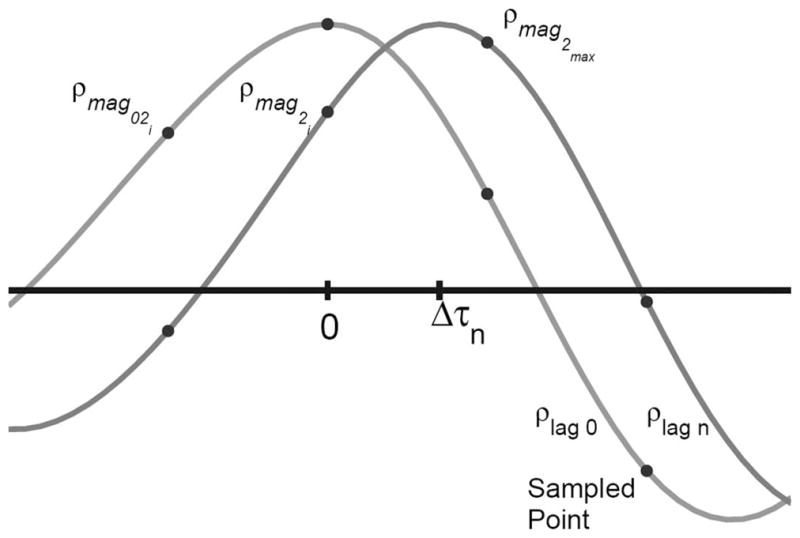
The figure demonstrates the bulk translation of the cross-correlation function (and the tissue scatterers) between the cross-correlation function with no time lag between the correlated signals and lag N between the 2 signals. It can be seen in the figure that the lag 0 cross-correlation is not symmetric and therefore not an autocorrelation function. The peak of the lag 0 cross-correlation will always be at 0. The peak of the lag N cross-correlation will be at Δ_τ, which will likely be between 2 sampled points. The sampled points that are used in the grid slopes subsample estimator are labeled in the figure and correspond to the points indicated in (5).

D. Methods: Phantom Validation

To validate 3-D motion tracking and test the limits of the chosen algorithm, a custom translation stage was constructed to perform phantom experiments with known translation distances and directions through 3-D space. In addition to the translation stage, an accompanying calibration phantom was also constructed.

The stage consisted of a linear translation stage and 2 rotational stages positioned orthogonally to each other. The translation stage was a 2-in. compact translation stage (Thorlabs, Newton, NJ). The 2 rotational stages were continuous rotation mounts (Thorlabs). The rotation stages allowed the transducer to be rotated around the transducer’s lateral and axial axes. By adjusting the rotation about the axial axis, different fixed ratios of lateral versus elevational motion could be created with a single linear translation stage. The translation stage was designed to be portable.

A calibration phantom was designed to ensure transducer orientation before imaging the speckle-generating phantom. The calibration phantom was an acrylic block. In the top of the block was a 4 × 4 grid of pins with 1-cm spacing in the lateral and elevational dimensions. The pins tip width was 37 ± 10 μm. (The pins acted as point targets for the lateral and elevational dimensions. The cross-sectional area of the pin tips was 3 orders of magnitude less than the cross-sectional area of the lateral-elevational point spread function.)

The calibration phantom and an accompanying calibration block were used to orient the translation stage for lateral motion. The orientation was accomplished by observing an ultrasonic C-mode image of the point targets. The point targets were aligned along the lateral and elevational dimensions of the transducer. Alignment along of the grid was accomplished visually, and for the duration of the experiment all angles were referenced relative to the calibration angle, which was defined as purely lateral transducer motion. The other 2 transducer orientations for which data were acquired were 22.5° and 45° rotated relative to pure lateral motion. The translation stage was translated in increments of 100 μm, and the first millimeter of translation steps were reported.

Speckle tracking was performed at an 8-cm range because this was the depth of transmit focus used when acquiring the in vivo cardiac data sets and is a realistic transmit depth for cardiac imaging. The kernel size was 2.2 × 2.8 × 2.8 mm for the axial, lateral, and elevational dimensions, respectively (2 beams in both the lateral and elevational kernel dimensions). The search region dimensions were 3.4 × 7 × 7 mm. The entire volume acquired for each transducer position was 20° × 18° and represented a grid of 4 × 3 transmit groups. The 4 × 3 grid of transmit beams was centered about the transducer’s axis (allowing for the use of the paraxial approximation). For each of the transducer’s translatory positions, 32 volumes were acquired and averaged offline. Additionally, data were acquired at 3 independent regions of a speckle-generating phantom providing 36 independent speckle realizations for each case.

All displacement estimates were postprocessed to remove peak hops in the axial direction and pixel hops in the lateral and elevational dimension. Axial peak hopping artifacts were removed by eliminating displacements in error by more than ± λ/2. Lateral and elevational pixel hopping artifacts were removed by eliminating any displacements in error by more than half the pixel spacing in a given dimension. In all cases, if a given dimension was found to have an error that was deemed to be due to pixel or peak hopping, the displacements–in all 3 dimensions–for that estimate were removed from the analyses. A threshold of 0.95 on the correlation level was applied.

E. Methods: Cardiac Speckle Tracking

Four 3-D in vivo cardiac ultrasound data sets were acquired with a ROI of 10° × 12° and a volume rate of 1000 Hz for 1 s. Three different kernel dimensions were analyzed. The average kernel sizes used were 1.2 × .85 × .85 mm, 2.2 × 1.7 × 1.7 mm, and 4.3 × 3.5 × 3.5 mm (corresponding to lateral and elevational beamwidths of 1, 2, and 4 beams, respectively) with slight variability in the lateral and elevational dimensions owing to depth dependency of beam width and different depths of the myocardium between acquisitions. The average depth of the distal wall of the left ventricle across the 4 data sets was 5.2 cm (and specifically 4.6 cm, 4.7 cm, 5.6 cm, and 5.9 cm). The search regions corresponding to each kernel were defined so that a velocity of 20 cm/s (or faster, based on discretization) was detectable for all dimensions. This allows for larger velocities than those seen in the literature for axial and circumferential motion; however, the tracking occurs in the transducer’s coordinate system and so it is not possible to know a priori more precise velocity maxima.

It can be difficult to determine peak and pixel hopping for in vivo tracking because the true displacement is rarely known. Therefore, a given displacement estimate was characterized as a peak or pixel hop if it met one of 2 criteria. The first possible criterion for categorizing a displacement estimate as a peak or pixel hop was the case when the displacement in a given dimension tracked to the edge of the search region. The second criterion for categorizing a displacement as a peak or pixel hop was the case when the 3-D velocity magnitude exceeded 22.9 cm/s. The threshold was based on the maximum diastolic velocity (mean + standard deviation) suggested from the results reported by Delfino et al. [6] assuming peak velocities occur simultaneously in all dimensions. The actual peak velocity magnitude calculated from the results in [6] was 17.9 m/s, and an additional 5 m/s was added in order not to disguise any methodologically based velocity differences. For both criteria, if a peak or pixel hop was found, all dimensions for that track were removed from analysis.

Because there were no known values for the in vivo cardiac motion tracking for any of the data acquired, 3 comparisons were performed to illuminate PRF dependent patterns in the data. The first 2 comparisons calculated the mean-absolute-difference (MAD) between the velocities throughout the cardiac cycle at a given volume rate against a constructed version at the same volume rate from the velocity estimates determined from the highest volume rate data. The first comparison compared motion estimates derived from downsampled data against the velocity estimates calculated from raw 1000-Hz volume rate data. The second comparison was identical, except the baseline estimate used the velocity estimates calculated from detected 1000-Hz volume rate data. The estimates derived from the highest volume rate data were used for comparisons because volume-to-volume displacement is smallest and volume-to-volume correlation is highest. Low displacement and high correlation tracking is expected to produce accurate motion estimates based on literature results [63] and the phantom results that will be shown.

The data used for comparison were created from the baseline velocity estimates from high frame rate data by low-pass filtering the velocity estimates with a rectangular window with unity amplitude and length N and then decimating by a factor of N where

$$N=\frac{F_{\text{high}}}{F_{\text{low}}}.$$ (7)

For the comparisons in this work, N was always an integer, F_high was always 1000 Hz and the F_low was allowed to be frequencies between 50 and 1000 Hz, subject to the described integer restriction. The literature indicates that, for cardiac imaging with a volume rate of 1000 Hz, the data processed in the raw format should perform better axially and nearly identically in the other 2 dimensions [33], [42]. However, despite the expectation that the 1000-Hz volume rate raw data should have the most accurate velocity estimates, it is necessary to compare raw data against constructed data detected and vice versa to avoid issues with data correlation. The third and final analysis was a direct comparison between velocity estimates derived from raw versus detected data at a given volume rate.

The comparisons were performed using data from 4 different in vivo data sets from the stated individual. All data used for the comparisons were taken from spatially independent kernels that remained within the myocardium through the entire cardiac cycle. Thirty-two independent kernels were realizable for the smallest kernel dimension, 24 for the mid-sized kernel, and 8 spatially independent kernels for the largest kernel. For the small and mid-sized kernels tracked at a volume rate of 67 Hz or below, only 16 and 12 independent kernels, respectively, were available for comparisons. For the largest kernel dimensions, 8 independent kernels were always available for comparison.

F. Methods: Cyclical Cardiac Speckle Stability

3-D in vivo cardiac ultrasound data were acquired with an ROI of 5° × 6°, and a 200-Hz volume rate for 5 s. The approximate kernel dimensions for performing the normalized cross-correlations were 2.2 mm × 1.7 mm × 1.7 mm. The search region was defined as the full extent of the transmit event (a 30-to-1 parallel receive beam group) within which a given kernel was defined.

Within these data sets, kernels–originating clearly within slow-filling diastole or systole as defined by M-mode inspection–were chosen and then the chosen kernels were used as the tracking kernel for all 5 s of discrete time lags.

The analysis conducted for this experiment contrasts with normal tracking where a kernel is usually only tracked across a small temporal lag. The process is expressed as

$${\mathrm{\Phi }}_n(m)=max\mid {\rho }_{n+m}(t,x,y)\mid ,\forall m.$$ (8)

The correlation values reported did not undergo sub-sample interpolation or any other filtering process.

III. Results

A. Results: Phantom Translation

The qualitative calibration of the transducer’s orientation can be seen in the C-mode image in Fig. 3. The large artifact in the lower right of the pin grid was a reflection that could not be removed. After calibration and data acquisition with known translation, 3-D speckle tracking using the described algorithm was performed. The results of speckle tracking can be seen in Fig. 4, where the rotations of the point spread function are 0°, 22.5°, and 45°. The agreement of the tracked and predicted values is generally within the range of the standard deviation. The standard deviations for the lateral and elevational tracking are within the expected jitter magnitude for tracking nonaxial displacements [33], [64].

Fig. 3.

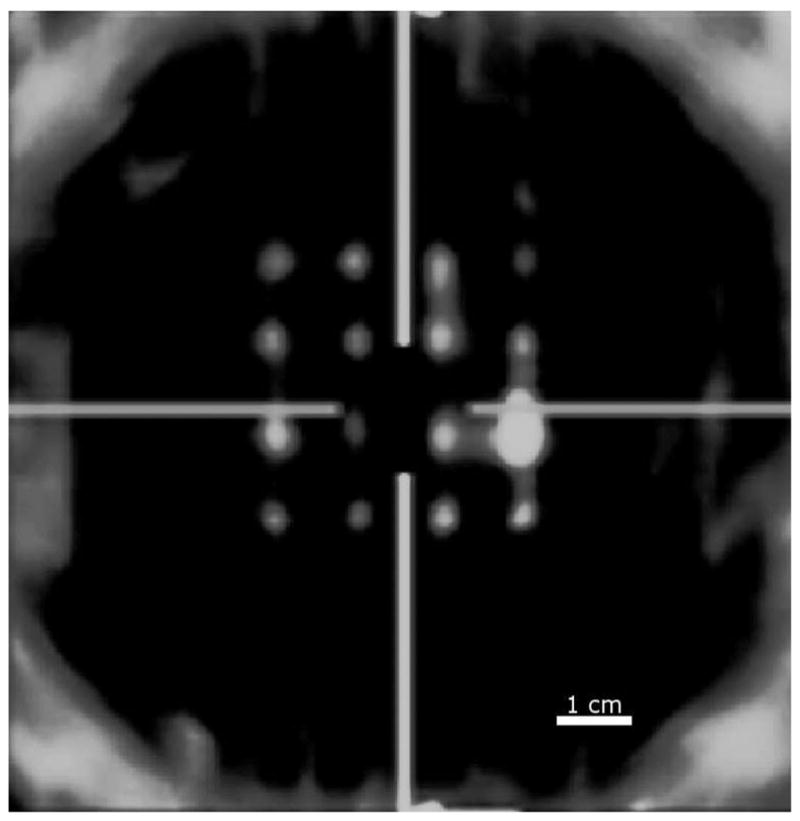
The figure shows a screen shot of the C-mode image at the depth of the pins. The image demonstrates the qualitative calibration of the translation stage before any phantom data were acquired. The horizontal lines shows the lateral orientation of the transducer, and the vertical lines show the elevational orientation of the transducer.

Fig. 4.

This figure shows the results of 3-D speckle tracking in a phantom with known translatory distances. The rows indicate the perceived rotation of the translation direction based on rotation of the transducer. The tracking dimensions are sorted by column. The kernel size for the phantom tracking was 2.2 × 2.8 × 2.8 mm. Each plot shows the mean and standard deviation for each tracking location.

B. Results: 3-D In Vivo Cardiac Displacement Tracking

The plots shown in Fig. 5 show direct comparison of same volume rate tracks from raw and detected methods. These plots indicate that, for the axial dimension, the relative performance of raw and detected tracking methods is constant at volume rates greater than about 100 Hz, allowing for some dependency on kernel size. The constant performance plateau degrades sooner for the smaller kernel.

Fig. 5.

The 3 figures show direct mean-absolute-difference comparisons of raw and detected velocity estimates for all 3 dimensions for each volume rate used for displacement estimation. The kernel sizes are denoted by small, medium, and large, which correspond to mean kernel sizes of 1.2 × .85 × .85 mm, 2.2 × 1.7× 1.7 mm, and 4.3 × 3.5 × 3.5 mm, respectively. The search limits refer to the volume rate where a full 20-cm/s velocity can no longer be tracked in the lateral or elevational dimension. (The position of the error bars and the search limits are slightly offset for legibility.)

The collection of plots shown in Figs. 6 and 7 present the MAD between the velocity estimated from raw and detected data. Fig. 6 shows the MAD for raw and detected data compared against velocities estimated from raw, 1000-Hz volume rate data. Fig. 7 shows the MAD comparison between the velocities calculated using 2 data types against velocities calculated using detected 1000-Hz volume rate data.

Fig. 6.

Raw echo reference. This series of figures shows the mean-absolute-difference comparison of raw and detected data types compared against raw echo data tracked at a volume rate of 1000 Hz. Figures are shown for the motion estimates for all 3 dimensions and for the 3 kernel sizes (1.2 × .85 × .85 mm, 2.2 × 1.7 × 1.7 mm, and 4.3 × 3.5 × 3.5 mm). The percent of false peak detection is shown for volume rates of 200 Hz and above. The light gray lines show the data from all the kernels used for the analysis and show that the mean trend is comparable to trends seen from individual kernels. The error bars showing the standard deviations are slightly offset for viewing clarity, and for the same reason, the error bars for the 83- and 111-Hz volume rates have been removed.

Fig. 7.

Detected echo reference. This series of figures shows the mean-absolute-difference comparison of raw and detected data types compared against detected echo data tracked at a volume rate of 1000 Hz. Figures are shown for the motion estimates for all 3 dimensions and for the 3 kernel sizes (1.2 × .85 × .85 mm, 2.2 × 1.7 × 1.7 mm, and 4.3 × 3.5 × 3.5 mm). The percent of false peak detection is shown for volume rates of 200 Hz and above. Additionally, the light gray lines show the data from all the kernels used for the analysis and show that the mean trend is comparable to trends seen from individual kernels. The error bars showing the standard deviations are slightly offset for viewing clarity, and for the same reason, the error bars for the 83- and 111-Hz volume rates have been removed.

In addition to the quality of the estimates, peak and pixel hopping is also a major quality factor when determining optimum tracking. The percentage of peak or pixel hops for the different cases is shown in Fig. 8. Peak and pixel hopping are not distinguished in the figure, and the percentage represents the number of times a peak or pixel hop occurs in at least one of the 3 tracked dimensions for a given estimate. There was less hopping when tracking is performed with raw data for the 2 smallest kernels. Larger kernels showed less peak and pixel hopping as well.

Fig. 8.

Peak and pixel hopping is shown as a function of volume rate. The 3 kernels sizes (1.2 × .85 × .85 mm, 2.2 × 1.7 × 1.7 mm, and 4.3 × 3.5 × 3.5 mm) are compared as well as the 2 data types (raw and detected).

Direct comparison between the in vivo and phantom results is difficult. One of the primary reasons comparison is difficult is the difference in expected estimation variance in the lateral and elevational dimensions due to the change in F/# over depth for cardiac imaging. The lateral and elevational variance has been shown to be closely modeled as 40(f/#)² [54]. The phantom data was tracked near 8 cm, while the left ventricle free wall was between 4 and 5 cm.

C. Results: In Vivo Cardiac Displacement Spatiotemporal Correlation

Additional qualitative metrics of motion tracking are demonstrated in the following figures, which show spatiotemporal correlation of the data and the tracking algorithm.

The first set of figures, Fig. 9, shows the magnitude of the zero-lag point of the normalized cross-correlation as a function of time and a matched M-mode image. In this case, a constant kernel was used to track the motion at all time points. A kernel originating during the slow filling portion of diastole as indicated by the M-mode data, and the rapid contraction of systole were both defined. The plots show the correlation across multiple heart cycles. There data were acquired with a volume rate of 200 Hz for 5 s. The results clearly show the cyclical nature of the speckle through 3-dimensions throughout the cardiac cycle. Additionally, the results show the relative stability and slow mobility of the scatterers during slow-filling diastole and the rapid decorrelation of the scatterers during systole. Finally, there is a consistent recorrelation of the scatterers as the heart passes through the phase of the cardiac cycle where each kernel originated.

Fig. 9.

Cardiac speckle correlation over several cardiac cycles is shown. The first figure shows the peak magnitude of the correlation function through time of a kernel originating in systole. The second figure shows the same thing except with a kernel originating during the slow filling portion of diastole. Third and finally, the matched M-mode data are shown.

In addition to the cyclical speckle stability just shown, the temporal reproducibility of complex spatial displacement patterns between cardiac cycles can be seen in Fig. 10 and can also be considered a qualitative metric of tracking performance. The figure shows the cumulative summation of the displacements tracked from a single location through 2 cardiac cycles. It should be noted that pixel-hopping artifacts were diminished with a 5-point median filter before cumulative summation, and the data were acquired at a 200-Hz volume rate. The results also show the better reproducibility of the motion in the axial dimension when compared with the other 2 dimensions. This is in part due to estimation jitter, but additionally, for parasternal views of the heart, transducer motion between cycles will have a more dominant effect on the lateral and elevational dimensions than the axial dimension.

Fig. 10.

The figures show different projection of the full 3-D displacement through 2 cardiac cycles. The displacement data were obtained from tracking with raw data. The kernel size for this data was 2.2 × 1.9 × 1.9 mm, and the volume rate was 200 Hz. The data were filtered with a 5-point median filter. Baseline drift was removed by subtracting the mean displacement before cumulatively summing the data. The 2 cardiac cycles displayed are distinguished by shades of gray. Velocity can be inferred from the displacement between spatial locations.

Another qualitative metric of performance is shown in Fig. 11, which shows the displacement through time of 2 spatially adjacent but independent kernels during a single cardiac cycle. The figure demonstrates the spatial stability of the data as well as the proposed algorithm’s ability to track the motion. No algorithm was applied to correct for peak hopping before cumulative summation. The images show the spatial reproducibility of fine motion, but also the effect of peak hopping and jitter as the positions of the 2 kernels appear to diverge throughout the cardiac cycle.

Fig. 11.

The series of figures shows cumulative displacement for 2 spatially independent kernel positions. The kernel size for these data was 2.2 × 1.7 × 1.7 mm, and the volume rate was 1000 Hz. The data were not filtered or baseline corrected. The drift—from the algorithm or transducer motion—is evident as well as peak/pixel hops. The kernels used were separated laterally by 1.7 mm. The kernels are distinguished by shades of gray. Velocity can be inferred from the displacement between spatial locations.

IV. Discussion

Three-dimensional speckle tracking using raw data was validated with phantom experiments. The results of the phantom tracking validation demonstrate the basic accuracy of the proposed method for estimating motion in the lateral and elevational dimensions, which is particularly important because the grid-slopes algorithm had never been implemented for 3-D coarsely sampled data.

In addition to phantom results, results have been provided from in vivo cardiac motion tracking. Because the in vivo tracking results lack a known value, the discussion for these results—which proceeds below—will progress deliberately to determine clearly appropriate inferences from the data. The 3 comparisons will be discussed: the effect of data type (raw or detected) when compared with the same data type, the effect of comparing raw or detected data against the alternative data type, and comparing velocity estimates of both data types from the same volume rate.

The following discussion pertains to tracking results shown in Fig. 6 and Fig. 7. When the acquired cardiac data are tracked in a given form (raw or detected) and compared against the same data format tracked at a lower volume rate, there is a decrease in the MAD as a function of increasing volume rate. The results for the MAD comparison for volume rates lower than about 100 to 200 Hz matches well with the MAD comparison between opposite data types (raw compared with detected and vice versa). However, for all dimensions of comparison, there is a decrease in the value of the MAD as the volume rate increases from 200 Hz to 1000 Hz. This trend could be misleading if any given figure were to be considered alone. (For example, it could be erroneously inferred that both detected and raw data types each track better than the other.) However, the decrease in the MAD comparison between low volume rate data and high volume rate data of the same type is in actuality a distraction. There is too much direct correlation of the displacement estimates owing to the volume-to-volume speckle stability at such high volume rates. Therefore, there is an overestimation of the similarity between estimates derived from the same data type. Although it is necessary to have correlation between volumes to use speckle-tracking methods, the combination of correlated speckle and the use of the same data type for comparison results in difficult interdependencies, which make fair inferences about tracking behavior difficult.

More interesting than the results from direct data type comparisons are the comparisons across data types (raw compared with detected and vice versa), which can be seen in Figs. 6 and 7. Both of the cross data comparisons use the highest volume rate, 1000 Hz, velocity estimates as a best case for comparisons. These comparisons show a general trend of little to no change beyond a given threshold. The threshold is kernel specific. The smallest kernel size has an estimation performance threshold near 330 Hz. The 2 larger kernels have estimation performance threshold that are lower, 150 to 200 Hz and 75 to 100 Hz for the medium and large kernels, respectively. Additionally, the stated values for the performance threshold are approximate, because the performance threshold is different for velocity estimates along the axial dimension when compared with the lateral and elevational dimension, and there is a variation between the raw and detected results. The term estimation performance is used to indicate that results presented in Figs. 6 and 7 demonstrate the point where an increase in volume rate has diminishing returns for improved estimation of displacement. There are other quality factors of performance, like peak and pixel hopping, which will be discussed later. However, to make the effects of estimation accuracy and pixel hopping more comparable, several pixel-hopping rates have been shown alongside the MAD values. Finally, the largest kernel does not seem to exhibit the same level of diminishing returns for estimates in the lateral and elevational dimensions when the raw echo data are used for comparison, shown in Fig. 6. However, the lateral and elevational dimensions demonstrate the same diminishing returns as a function of volume rate when examined in Fig. 5, which will be discussed next.

The final point of discussion pertaining to the results on the performance of velocity estimation as a function of volume rate examines the direct comparison of raw and detected data. This comparison contrasts with the previously discussed comparison where the velocity estimates were always compared against a constructed version of high volume rate data. The comparison shown in Fig. 5 presents the direct comparison, which has many similarities to Figs. 6 and 7. These figures also demonstrate a diminishing return, but the effect is subtler. What these figures primarily show is the range over which velocity estimates derived from raw and detected data have a stable relationship. The lateral and elevational dimensions, generally, show that there is little difference between using raw and detected for any volume rate. There may be some change in relative performance for these tracking dimensions, but the variation of the data would makes this statement tenuous. The relationship for tracking along the axial dimension is slightly more dynamic. The most obvious case is for the smallest kernel for axial tracking, which shows that there is a large difference between raw and detected methods until the volume rate reaches 333 Hz. A similar but less dramatic trend can be seen for axial tracking with medium and large kernel.

One thing that should not be inferred from the results is that the performance of the velocity estimates from raw and detected data converge somewhere near 100 Hz. This could be inferred from inspection of only the mean value in Figs. 6 and 7. Inferring that the performance of the raw and detected data converge would be ignoring Fig. 5, which may show that the velocity estimates are actually divergent when tracking with raw versus detected data at frame rates less than 100 Hz. One clear benefit of tracking cardiac motion above volume rates of 200 Hz is the decrease in peak/pixel hopping with increasing volume rate. This trend has been shown in Fig. 8 and demonstrates that pixel hopping continues to improve as a function of volume rate longer than the MAD velocity estimation comparisons. The pixel hopping shown in Fig. 8 is probably overstated due to the large search regions used, however, the high pixel hopping could also be attributed to the extra degree of freedom provided by the third dimension of motion tracking. Most speckle-tracking algorithms do employ some method to correct pixel hopping, but literature-based methods for this are notoriously vague. There is at least one clearly defined method to reduce pixel hopping proposed by Lubinski et al. [51]. Even this paper does not clearly define what to do with pixel hops that remain or the resulting effect of correcting them.

The tracking quality measures examined show that larger kernels demonstrate less difference between tracking with raw and detected data and have fewer pixel hops than smaller kernels. The improvement of large kernels over small is mitigated by the loss in tracking resolution, which results in averaging over motion gradients that can represent important diagnostic information [56]. In fact, it can be the case that larger kernels will track the true displacement worse than smaller kernels, but the analysis presented here only makes comparisons between kernels of identical size, so it is not possible to determine at what point internal motion gradients become detrimental to the benefits of tracking with a larger kernel. The resulting trade-off between the spatial resolution of motion tracking and the accuracy of motion tracking does not present an obvious decision and is generally application specific.

The results shown here cannot immediately be extrapolated to other methods of tracking, such as optical flow. However, the results are likely valid for cost functions similar to normalized cross-correlation such as the sum-absolute-difference or sum-squared-difference cost functions [65].

The trends in the results have implications for 3-D cardiac strain and strain rate imaging. However, it is not known how the results in this paper will affect clinical strain and strain rate imaging because of proprietary manufacturer algorithms and because strain and strain rate imaging are still clinically limited to 2-D. As an example, papers have cited either the necessity of above-average quality images to strain and strain rate analysis [66] or have removed poor quality images from the analysis (.21% of a general population study using the tissue Doppler method) [67]. In any case, the minimum required level of image quality and tracking performance (in terms of SNR, estimation precision, peak/pixel hopping, e.g.) to perform strain and strain analyses in 2-D, let alone 3-D, is not clear.

Despite the current method of examining strain and strain rate imaging offline, eventually the challenge with 3-D speckle tracking may be to implement fully 3-D speckle tracking in a clinical setting. There are several challenges to implementing 3-D strain and strain rate imaging in real time. The first challenge is acquiring 3-D data at an adequate rate. Currently, strain imaging is acquired at modest frame rates, but the results indicate that volume rates of 200 Hz or higher may benefit tracking performance. The requirements for obtaining a full 90° lateral sector scan with an amount of elevation data sufficient for 3-D speckle tracking (approximately 5°) does not seem trivial. However, for cardiac strain imaging, acquiring a full lateral cross section with enough elevation data for tracking in all 3 dimensions is an immediately realizable imaging sequence on some commercial volumetric ultrasound scanners. Assuming an imaging depth of 16 cm, a sound speed of 1540 m/s, and a receive beam sequence with 1° sampling in both the lateral and elevational dimensions, a 90° × 5° field of view could be obtained at a volume rate of 200 Hz if at least 19 beams could be acquired in parallel. This hypothetical sequence is not implementable on most scanners, but a slight decrease in the field of view or volume rate could increase the number of scanners capable of running high-quality 3-D speckle tracking sequences.

In addition to the difficulties of acquiring raw volumetric data, the second challenge to real-time 3-D motion tracking is its computational expense. Current clinical applications of cardiac strain and strain rate imaging are performed offline. The proposed algorithm may be too inefficient for real-time applications. However, if detected data was determined to be accurate enough, the current algorithm could be simplified by employing a sum-squared-error or sum-absolute-difference cost function. Strategies for accelerating the proposed cost function (normalized cross-correlation) have been presented by Chen et al. [36].

Generally, the best method for tracking volume data remains an open question. This statement applies to both the context of the trade-offs between tracking detected and raw data as well as the best methods for tracking each type of data. The trade-off between detected and raw data tracking has been well established by several investigators [41], [42] The trade-off between the use of the 2 data types will in many cases come down to the available technology and the ability to acquire and process raw data.

There are other variables that affect 3-D cardiac speckle tracking that were not tested here, but that have been explored by Meunier in 3-D tracking simulations [41]. Two such variables that Meunier explored were the system’s point spread function and the transmit center frequency. This paper did not examine either of these variables. However, some of the performance variability seen in the results may be directly attributable to the point spread function’s dependence on depth for phased-array probes. In general, for phased-array cardiac imaging, tight point spread functions are difficult to come by due to small aperture size. Additionally, because the interrogation frequency is inversely proportion to the size of the point spread function, these 2 effects are not complimentary. Therefore, to achieve high-performance cardiac speckle tracking, it will be desirable to optimize this trade-off. Both of the discussed effects will also directly affect the rate of speckle decorrelation. Optimizing the imaging parameters for cardiac tracking will not be a trivial task.

V. Conclusion

Three-dimensional speckle tracking on raw data has been demonstrated in both phantom and in vivo scenarios. Although the clinical data are preliminary, they show that in vivo 3-D speckle tracking with raw data is possible with the current, available state of ultrasound technology, and the spatial and temporal repeatability is consistent with high-quality speckle tracking.

The results demonstrate performance trends as a function of the volume rate. Displacement estimation and pixel hopping were shown to decrease as the sampling rate increases. When comparing the trends of displacement estimation and pixel hopping, displacement estimation shows clear diminishing returns as a function of volume rate well before pixel-hopping performance starts to plateau.

The presented results also clearly demonstrate the relationship between kernel size and performance for 3-D speckle tracking. Although there may be an asymptotic relationship between kernel size and performance similar to the one seen with volume rate, not enough kernel sizes were explored to illuminate this potential trend fully.

Finally, it is clear from the results that axial estimation is much less sensitive to kernel size when compared with the lateral and elevational dimensions.

The arrival of 3-D speckle tracking on raw in vivo data should answer many long-standing questions within the field and introduce a plethora of new possibilities for future investigation.

Biographies

Brett C. Byram is a graduate student in the Biomedical Engineering Department at Duke University, Durham, NC, working towards the Ph.D. degree. He received the B.S. degree in Biomedical Engineering and Math in 2004 from Vanderbilt University, Nashville, TN. He is a graduate of the National Outdoor Leadership School and a member of the Society of Duke Fellows. His ultrasound research interests include beamforming and motion estimation.

Greg Holley photograph and biography not available at time of publication.

Douglas M. Giannantonio was born in Med-ford, NJ in 1987. He is expected toreceive his B.S.E. degree in biomedical engineering from Duke University in May 2010. He is an undergraduate researcher through the Pratt Engineering Fellows Program. His current research is acoustic radiation force based imaging for cardiac applications

Gregg E. Trahey (S’83–M’85) received the B.G.S. and M.S. degrees from the University of Michigan, Ann Arbor, MI, in 1975 and 1979, respectively. He received the Ph.D. degree in biomedical engineering in 1985 from Duke University, Durham, NC. He served in the Peace Corps from 1975 to 1978, and was a project engineer at the Emergency Care Research Institute in Plymouth Meeting, PA, from 1980 to 1982. He is a professor with the Department of Biomedical Engineering, Duke University. He is conducting research in adaptive phase correction, radiation force imaging methods, and 2-D flow imaging in medical ultrasound.

References

- 1.Dandel M, Hetzer R. Echocardiographic strain and strain rate imaging–clinical applications. Int J Cardiol. 2009;132(1):11–24. doi: 10.1016/j.ijcard.2008.06.091. [DOI] [PubMed] [Google Scholar]
- 2.Chaitman BR, DeMots H, Bristow JD, Rösch J, Rahimtoola SH. Objective and subjective analysis of left ventricular angiograms. Circulation. 1975 Sep;52:420–425. doi: 10.1161/01.cir.52.3.420. [DOI] [PubMed] [Google Scholar]
- 3.Gallagher KP, Matsuzaki M, Osakada G, Kemper WS, Ross J. Effect of exercise on the relationship between myocardial blood flow and systolic wall thickening in dogs with acute coronary stenosis. Circ Res. 1983 Jun;52:716–720. doi: 10.1161/01.res.52.6.716. [DOI] [PubMed] [Google Scholar]
- 4.Urheim S, Edvardsen T, Torp H, Angelsen B, Smiseth OA. Myocardial strain by doppler echocardiography validation of a new method to quantify regional myocardial function. Circulation. 2000 Sep;102:1158–1164. doi: 10.1161/01.cir.102.10.1158. [DOI] [PubMed] [Google Scholar]
- 5.Wedeen VJ. Magnetic resonance imaging of myocardial kinematics. Technique to detect, localize, and quantify the strain rates of the active human myocardium. Magn Reson Med. 1992 Sep;27:52–67. doi: 10.1002/mrm.1910270107. [DOI] [PubMed] [Google Scholar]
- 6.Delfino JG, Johnson KR, Eisner RL, Eder S, Leon AR, Oshinski JN. Three-directional myocardial phase-contrast tissue velocity mr imaging with navigator-echo gating: In vivo and in vitro study. Radiology. 2008 Mar;246(3):917–925. doi: 10.1148/radiol.2463062155. [DOI] [PubMed] [Google Scholar]
- 7.Petersen SE, Jung BA, Wiesmann F, Selvanayagam JB, Francis JM, Hennig J, Neubauer S, Robson MD. Myocardial tissue phase mapping with cine phase-contrast mr imaging: Regional wall motion analysis in healthy volunteers. Radiology. 2006 Mar;238(3):816–826. doi: 10.1148/radiol.2383041992. [DOI] [PubMed] [Google Scholar]
- 8.Markl M, Schneider B, Hennig J, Peschl S, Winterer J, Krause T, Laubenberg J. Cardiac phase contrast gradient echo MRI: measurement of myocardial wall motion in healthy volunteers and patients. Int J Card Imag. 1999;15(6):441–452. doi: 10.1023/a:1006355106334. [DOI] [PubMed] [Google Scholar]
- 9.Meyer RA. History of ultrasound in cardiology. J Ultrasound Med. 2004 Jan;23:1–11. doi: 10.7863/jum.2004.23.1.1. [DOI] [PubMed] [Google Scholar]
- 10.Theroux P, Franklin D, Ross J, Jr, Kemper WS. Regional myocardial function during acute coronary artery occlusion and its modification by pharmacologic agents in the dog. Circ Res. 1974 Dec;35:896–908. doi: 10.1161/01.res.35.6.896. [DOI] [PubMed] [Google Scholar]
- 11.Bijnens B, Claus P, Weidermann F, Strotmann J, Sutherland GR. Investigating cardiac function using motion and deformation analysis in the setting of coronary artery disease. Circulation. 2007 Nov;116:2453–2464. doi: 10.1161/CIRCULATIONAHA.106.684357. [DOI] [PubMed] [Google Scholar]
- 12.Meier GD, Ziskin MC, Santamore WP, Bove AA. Kinematics of the beating heart. IEEE Trans Biomed Eng. 1980;BME-27(6):319–329. doi: 10.1109/TBME.1980.326740. [DOI] [PubMed] [Google Scholar]
- 13.Meier GD, Bove AA, Santamore WP. Contractile function in canine right ventricle. Am J Physiol Heart Circ Physiol. 1980;239(6):H794–H804. doi: 10.1152/ajpheart.1980.239.6.H794. [DOI] [PubMed] [Google Scholar]
- 14.Shechter G, Devernay F, Coste-Manière E, Quyyumi A, McVeigh ER. Three-dimensional motion tracking of coronary arteries in biplane cineangiograms. IEEE Trans Med Imaging. 2003 Apr;22(4):493–503. doi: 10.1109/TMI.2003.809090. [DOI] [PMC free article] [PubMed] [Google Scholar]
- 15.Shechter G, Resar JR, McVeigh ER. Displacement and velocity of the coronary arteries: Cardiac and respiratory motion. IEEE Trans Med Imaging. 2006 Mar;25(3):369–375. doi: 10.1109/TMI.2005.862752. [DOI] [PMC free article] [PubMed] [Google Scholar]
- 16.Braun H, Hauck A. Tomographic reconstruction of vector fields. IEEE Sig Proc. 1991;39(10):464–471. [Google Scholar]
- 17.Yu H, Wang G. A general scheme for velocity tomography. Signal Processing. 2008 May;88:1165–1175. doi: 10.1016/j.sigpro.2007.11.007. [DOI] [PMC free article] [PubMed] [Google Scholar]
- 18.Moran PR. A flow velocity zeumatographic interlace for NMR imaging in humans. Magn Reson Imaging. 1982;1(4):192–203. doi: 10.1016/0730-725x(82)90170-9. [DOI] [PubMed] [Google Scholar]
- 19.van Dijk P. Direct cardiac NMR imaging of heart wall and blood-flow velocity. J Comput Assist Tomogr. 1984 Jun;8:429–436. doi: 10.1097/00004728-198406000-00012. [DOI] [PubMed] [Google Scholar]
- 20.Ozturk C, Derbyshire A, McVeigh ER. Estimating motion from MRI data. Proc IEEE. 2003;91(10):1627–1648. doi: 10.1109/JPROC.2003.817872. [DOI] [PMC free article] [PubMed] [Google Scholar]
- 21.Li G, Citrin D, Camphausen K, Mueller B, Burman C, Mychalczak B, Miller RW, Song Y. Advances in 4D medical imaging and 4D radiation therapy. Tech Canc Res Treat. 2008;7(1):67–81. doi: 10.1177/153303460800700109. [DOI] [PubMed] [Google Scholar]
- 22.Embree P, O’Brien JWD. The accurate ultrasonic measurement of volume flow of blood by time domain correlation. Proc. 1985 IEEE Ultrasonics Symp; pp. 963–966. [Google Scholar]
- 23.Kasai C, Namekawa K, Koyano A, Omoto R. Real-time two-dimensional blood flow imaging using an autocorrelation technique. IEEE Trans Ultrason Ferroelectr Freq Control. 1985 May;32(3):458–464. [Google Scholar]
- 24.Loupas T, Powers JT, Gill RW. An axial velocity estimator for ultrasound blood flow imaging, based on a full evaluation of the Doppler equation by means of a two-dimensional autocorrelation approach. IEEE Trans Ultrason Ferroelectr Freq Control. 1995 Jul;42(4):672–688. [Google Scholar]
- 25.Trahey GE, Allison JW, Ramm OTV. Angle independent ultrasonic flow detection of blood flow. IEEE Trans Biomed Eng. 1987 Dec;BME-34(12):965–967. doi: 10.1109/tbme.1987.325938. [DOI] [PubMed] [Google Scholar]
- 26.Meunier J, Bertrand M. Ultrasonic texture motion analysis: Theory and simulation. IEEE Trans Med Imaging. 1995;14(2):293–300. doi: 10.1109/42.387711. [DOI] [PubMed] [Google Scholar]
- 27.Shiina T, Doyley MM, Bamber JC. Strain imaging using combined rf and envelope autocorrelation processing. Proc. 1996 IEEE Ultrasonics Symp; pp. 1331–1336. [Google Scholar]
- 28.Cohn NA, Emelianov SY, Lubinski MA, O’Donnell M. An elasticity microscope. Part I: Methods. IEEE Trans Ultrason Ferroelectr Freq Control. 1997 Nov;44(6):1304–1319. [Google Scholar]
- 29.Yeung F, Levinson SF, Parker KJ. Multilevel and motion model-based ultrasonic speckle tracking algorithms. Ultrasound Med Biol. 1998 Mar;24:427–441. doi: 10.1016/s0301-5629(97)00281-0. [DOI] [PubMed] [Google Scholar]
- 30.Mikic I, Krucinksi S, Thomas JD. Segmentation and tracking in echocardiographic sequences: Active contours guided by optical flow estimates. IEEE Trans Med Imaging. 1998 Apr;17:274–284. doi: 10.1109/42.700739. [DOI] [PubMed] [Google Scholar]
- 31.Hein IA, O’Brien WD. Current time-domain methods for assessing tissue motion by analysis from reflected ultrasound echoes–a review. IEEE Trans Ultrason Ferroelectr Freq Control. 1993 Mar;40:84–102. doi: 10.1109/58.212556. [DOI] [PubMed] [Google Scholar]
- 32.Viola F, Walker WF. A comparison of the performance of time-delay estimators in medical ultrasound. IEEE Trans Ultrason Ferroelectr Freq Control. 2003 Apr;50:392–401. doi: 10.1109/tuffc.2003.1197962. [DOI] [PubMed] [Google Scholar]
- 33.Walker W, Trahey G. A fundamental limit on the performance of correlation-based phase correction and flow estimation techniques. IEEE Trans Ultrason Ferroelectr Freq Control. 1994 Sep;41:644–654. [Google Scholar]
- 34.Ramm OV, Smith S, Sheikh K. Real-time three-dimensional echocardiography. Proc. 61st Scientific Sessions of the American Heart Association (Circulation); Nov. 1988; p. II35. [Google Scholar]
- 35.Steele DD, Chenevert TL, Skovoroda AR, Emelianov SY. Three-dimensional static displacement, stimulated echo NMR elasticity imaging. Phys Med Biol. 2000 Jun;45:1633–1648. doi: 10.1088/0031-9155/45/6/316. [DOI] [PubMed] [Google Scholar]
- 36.Chen X, Xie H, Erkamp R, Kim K, Jia C, Rubin JM, O’Donnell M. 3-D correlation-based speckle tracking. Ultrason Imaging. 2005 Jan;27:21–36. doi: 10.1177/016173460502700102. [DOI] [PubMed] [Google Scholar]
- 37.Bharat S, Fisher TG, Varghese T, Hall TJ, Jiang J, Madsen EL, Zagzebski JA, Lee FT., Jr Three-dimensional electrode displacement elastography using the siemens c7f2 Four-sight four-dimensional ultrasound transducer. Ultrasound Med Biol. 2008 Aug;34:1307–1316. doi: 10.1016/j.ultrasmedbio.2008.01.007. [DOI] [PMC free article] [PubMed] [Google Scholar]
- 38.Canals R, Lamarque G, Chatain P. Volumetric ultrasound system for left ventricle motion imaging. IEEE Trans Ultrason Ferroelectr Freq Control. 1999 Nov;46:1527–1538. doi: 10.1109/58.808877. [DOI] [PubMed] [Google Scholar]
- 39.de Jong N, Djoa KK, van der Steen AFW, Lancée CT, Kasprzak JD, Breburda C, Bom N. Real-time three dimensional data acquisition. Proc. 1998 IEEE Ultrasonics Symp; pp. 1843–1846. [Google Scholar]
- 40.Bashford GR, von Ramm OT. Speckle structure in three dimensions. J Acoust Soc Am. 1995 Jul;98:35–42. doi: 10.1121/1.413690. [DOI] [PubMed] [Google Scholar]
- 41.Meunier J. Tissue motion assessment from 3D echographic speckle tracking. Phys Med Biol. 1998 May;43:1241–1254. doi: 10.1088/0031-9155/43/5/014. [DOI] [PubMed] [Google Scholar]
- 42.Yu W, Yan P, Sinusas AJ, Thiele K, Duncan JS. Towards pointwise motion tracking in echocardiographic image sequences–comparing the reliability of different features for speckle tracking. Med Image Anal. 2006 Aug;10:495–508. doi: 10.1016/j.media.2005.12.003. [DOI] [PubMed] [Google Scholar]
- 43.Morsy AA, von Ramm OT. Flash correlation: A new method for 3-D ultrasound tissue motion tracking and blood velocity estimation. IEEE Trans Ultrason Ferroelectr Freq Control. 1999 May;46(3):728–736. doi: 10.1109/58.764859. [DOI] [PubMed] [Google Scholar]
- 44.Kuo J, von Ramm OT. Three-dimensional motion measurements using feature tracking. IEEE Trans Ultrason Ferroelectr Freq Control. 2008 Apr;55(4):800–810. doi: 10.1109/TUFFC.2008.714. [DOI] [PubMed] [Google Scholar]
- 45.Duan Q, Angelini ED, Herz SL, Ingrassia CM, Costa KD, Holmes JW, Homma S, Laine AF. Region-based endocardium tracking on real-time three-dimensional ultrasound. Ultrasound Med Biol. 2009 Feb;35:256–265. doi: 10.1016/j.ultrasmedbio.2008.08.012. [DOI] [PMC free article] [PubMed] [Google Scholar]
- 46.Crosby J, Amundsen BH, Hergum T, Remme EW, Langeland S, Torp H. 3-D speckle tracking for assessment of regional left ventricular function. Ultrasound Med Biol. 2009 Mar;35:458–471. doi: 10.1016/j.ultrasmedbio.2008.09.011. [DOI] [PubMed] [Google Scholar]
- 47.Linguraru MG, Vasilyev NV, Marx GR, Tworetzky W, Nido PJD, Howe RD. Fast block flow tracking of atrial septal defects in 4D echocardiography. Med Image Anal. 2008 Aug;12:397–412. doi: 10.1016/j.media.2007.12.005. [DOI] [PMC free article] [PubMed] [Google Scholar]
- 48.Shattuck DP, Weinshenker MD, Smith SW, von Ramm OT. Explososcan: A parallel processing technique for high speed ultrasound imaging with linear phased arrays. J Acoust Soc Am. 1984 Apr;75(4):1273–1282. doi: 10.1121/1.390734. [Online]. Available: http://link.aip.org/link/?JAS/75/1273/1. [DOI] [PubMed] [Google Scholar]
- 49.Üstüner K. Siemens Healthcare Sector, White Paper. 2008. High information rate volumetric ultrasound imaging. [Google Scholar]
- 50.Frey G, Chiao R. Siemens Healthcare Sector, White Paper. 2008. 4z1c real-time volume imaging transducer. [Google Scholar]
- 51.Lubinski MA, Emelianov SY, O’Donnell M. Speckle tracking methods for ultrasonic elasticity imaging using short-time correlation. IEEE Trans Ultrason Ferroelectr Freq Control. 1999 Jan;46(1):82–96. doi: 10.1109/58.741427. [DOI] [PubMed] [Google Scholar]
- 52.Pinton GF, Dahl JJ, Trahey GE. Rapid tracking of small displacements with ultrasound. IEEE Trans Ultrason Ferroelectr Freq Control. 2006 Jun;53:1103–1117. doi: 10.1109/tuffc.2006.1642509. [DOI] [PubMed] [Google Scholar]
- 53.Wagner RF, Smith SW, Sandrik JM, Lopez H. Statistics of speckle in ultrasound b-scans. IEEE Trans Sonics Ultrason. 1983;30(3):156–163. [Google Scholar]
- 54.Wear KA, Popp RL. Theoretical analysis of a technique for the characterization of myocardium contraction based upon temporal correlation of ultrasonic echoes. IEEE Trans Ultrason Ferroelectr Freq Control. 1987 May;34:368–375. doi: 10.1109/t-uffc.1987.26955. [DOI] [PubMed] [Google Scholar]
- 55.O’Donnell M, Skovoroda AR, Shapo BM, Emelianov SY. Internal displacement and strain imaging using ultrasonic speckle tracking. IEEE Trans Ultrason Ferroelectr Freq Control. 1994 May;41(3):314–325. [Google Scholar]
- 56.Friemel BH, Bohs LN, Nightingale KR, Trahey GE. Speckle decorrelation due to two-dimensional flow gradients. IEEE Trans Ultrason Ferroelectr Freq Control. 1998 Mar;45(2):317–327. doi: 10.1109/58.660142. [DOI] [PubMed] [Google Scholar]
- 57.Lai X, Torp H. Interpolation methods for time-delay estimation using cross-correlation method for blood velocity measurement. IEEE Trans Ultrason Ferroelectr Freq Control. 1999 Mar;46(2):277–290. doi: 10.1109/58.753016. [DOI] [PubMed] [Google Scholar]
- 58.Céspedes I, Huang Y, Ophir J, Spratt S. Methods for estimation of subsample time delays of digitized echo signals. Ultrason Imaging. 1995 Apr;17:142–171. doi: 10.1177/016173469501700204. [DOI] [PubMed] [Google Scholar]
- 59.Viola F, Walker WF. A spline-based algorithm for continuous time-delay estimation using sampled data. IEEE Trans Ultrason Ferroelectr Freq Control. 2005 Jan;52(1):80–93. doi: 10.1109/tuffc.2005.1397352. [DOI] [PubMed] [Google Scholar]
- 60.Pinton GF, Trahey GE. Continuous delay estimation with polynomial splines. IEEE Trans Ultrason Ferroelectr Freq Control. 2006 Nov;53:2026–2035. doi: 10.1109/tuffc.2006.143. [DOI] [PubMed] [Google Scholar]
- 61.Geiman BJ, Bohs LN, Anderson ME, Breit SM, Trahey GE. A novel interpolation strategy for estimating subsample speckle motion. Phys Med Biol. 2000 Jun;45:1541–1552. doi: 10.1088/0031-9155/45/6/310. [DOI] [PubMed] [Google Scholar]
- 62.Bohs LN, Geiman BJ, Anderson ME, Breit SM, Trahey GE. Ensemble tracking for 2d vector velocity measurement: Experimental and initial clinical results. IEEE Trans Ultrason Ferroelectr Freq Control. 1998 Jul;45(4):912–924. doi: 10.1109/58.710557. [DOI] [PubMed] [Google Scholar]
- 63.Walker W, Trahey G. A fundamental limit on delay estimation using partially correlated speckle signals. IEEE Trans Ultrason Ferroelectr Freq Control. 1995 Mar;42(2):301–308. [Google Scholar]
- 64.Lubinski MA, Emelianov SY, Raghavan KR, Yagle AE, Skovoroda AR, O’Donnell M. Lateral displacement estimation using tissue incompressibility. IEEE Trans Ultrason Ferroelectr Freq Control. 1996 Mar;43:247–256. doi: 10.1109/58.660158. [DOI] [PubMed] [Google Scholar]
- 65.Friemel BH, Bohs LN, Trahey GE. Relative performance of two-dimensional speckle-tracking techniques: Normalized correlation, non-normalized correlation and sum-absolute-difference. Proc. 1995 IEEE Ultrasonics Symp; pp. 1481–1484. [Google Scholar]
- 66.Pavlopoulos H, Nihoyannopoulos P. Strain and strain rate deformation parameters: From tissue doppler to 2d speckle tracking. Int J Cardiovasc Imaging. 2008 Jun;24:479–491. doi: 10.1007/s10554-007-9286-9. [DOI] [PubMed] [Google Scholar]
- 67.Kuznetsova T, Herbots L, Richart T, D’hooge J, Thijs L, Fagard RH, Herregods MC, Staessen JA. Left ventricular strain and strain rate in a general population. Eur Heart J. 2008;29(16):2014–2023. doi: 10.1093/eurheartj/ehn280. [DOI] [PubMed] [Google Scholar]