Real-time Dynamic Frequency and Shim Correction for Single-voxel MR Spectroscopy

Abstract

Subject motion during brain magnetic resonance spectroscopy (MRS) acquisitions generally reduces the magnetic field (B₀) homogeneity across the volume of interest, or voxel. This is the case even if prospective motion correction ensures that the voxel follows the head. We introduce a novel method for rapidly mapping linear variations in B₀ across a small volume using two-dimensional excitations. The new field mapping technique was integrated into a prospectively motion-corrected single-voxel ¹H MRS sequence. Interference with the MRS measurement was negligible and there was no penalty in scan time. Frequency shifts were also measured continuously, and both frequency and first-order shim corrections were applied in real time. Phantom experiments and in vivo studies demonstrated that the resulting motion- and shim-corrected sequence is able to mitigate line broadening and maintain spectral quality even in the presence of large-amplitude subject motion.

INTRODUCTION

Magnetic resonance spectroscopy (MRS) allows the non-invasive measurement of major metabolite concentrations in vivo. MRS scans typically require several minutes of averaging in order to obtain adequate signal-to-noise ratio (SNR). Therefore, patient motion, and the accompanying reduction in the quality and reliability of the resulting spectra (1), is relatively common. A number of methods have been proposed to correct motion-related artifacts in MRS, including techniques that perform a posteriori frequency- and phase-corrections (2–4) and those that track patient motion and perform real-time updates of voxel position and orientation (5–8).

Single-voxel spectroscopy sequences are well-suited to real-time corrections, since they typically have substantial “dead time” in each repetition (TR) period to allow for recovery of longitudinal magnetization. This spare time can be used to perform motion correction in real time, provided interference with the relaxation process is minimal. Several real-time motion compensation techniques for single-voxel MRS have been introduced in recent years, using MR-based navigators (5,6) as well as methods employing external systems, such as optical cameras (7,9). In previous work, we (5) and others (6) have demonstrated that a navigator-based motion correction scheme, appropriately integrated into an MRS sequence, can ensure the voxel remains stationary relative to the brain in the presence of subject motion. Since averages are acquired from the same anatomical region, the reproducibility of the measured metabolite concentrations is improved.

In addition to causing an ill-defined volume of interest, patient motion may degrade the magnetic field (B₀) homogeneity across the voxel, or “shim”. The B₀ homogeneity may be reduced directly via the motion of the susceptibility tensor field (which moves with the head), especially in regions near air/tissue interfaces, such as the frontal lobe. In addition, since the homogeneity of the B₀ field is highly optimized (i.e., shimmed) over the MRS voxel prior to the start of the scan, dynamic updates of the voxel position will often move it into a region of poorer shim.

Since the metabolites in proton spectra have closely spaced resonance frequencies, MRS requires a high degree of B₀ homogeneity to adequately resolve spectral peaks. Poor shim is associated with broadened spectral peaks and reduced accuracy of measured metabolite concentrations (10). Using motion-corrected MRS acquisitions, we have demonstrated that even moderate head movements can degrade spectral quality (5,11), which may confound quantification of metabolite concentrations. Further, shim changes during head movements are subject-dependent and difficult to predict, even if the motion is perfectly characterized (but see (12)). Thus, prospective motion correction for single-voxel MRS requires dynamic shimming in order to produce high-quality spectra.

In this paper we describe a novel method for rapidly measuring the B₀ field in an MRS voxel, and using the field distribution to perform first-order shim corrections in real time (“dynamic shimming”). Additionally, the center frequency of the VOI is measured and updated continuously. This is accomplished without appreciably reducing the SNR of the resulting spectra. We demonstrate that the combination of dynamic shimming and continuous frequency updates, together with real-time motion tracking, improves spectral quality and increases the reproducibility of metabolite concentrations in the presence of subject motion without increasing scan time.

METHODS

MR Methods

Dynamic shimming and frequency adjustment were implemented in a standard short echo time point-resolved spectroscopy (PRESS) (13) sequence (echo/repetition time (TE/TR) = 35 / 3000ms, bandwidth = 1200Hz, 32 averages, 20×20×20mm³ voxel). Figure 1 outlines how the vendor-supplied pulse sequence was modified. First, at the beginning of each TR period, an image-based motion navigator was added to track head movements, as described previously (5) (“Motion Nav” module in Fig. 1). Immediately following the motion navigator and prior to water suppression, a new module was inserted to determine linear shim corrections (“Dyn Shim” Fig. 1). Furthermore, the water suppression block (“WS” in Figure 1) was modified to enable retrospective frequency and phase corrections (4).

FIG. 1.

The gradient and RF waveforms for a single MRS average (blocks), as well as real-time data flow (arrows). Subscripts index the MRS averages. The frequency correction measured during the PRESS readout (green) is applied immediately so that the motion navigators for the following average (blue) are on-resonance. Note that “shim corrections” (red) includes the zero-order correction, i.e., the frequency shift resulting from 1^st order shim corrections. Abbreviations used: “Dyn Shim”=dynamic shimming/B₀ mapping, “Motion Nav”=PROMO-based motion navigator, “WS”=weak water suppression with phase cycling.

Several feedback loops were implemented to enable these dynamic adjustments. First, tracking data from the motion navigator were used to adjust the positions and orientations of subsequent dynamic shim and PRESS modules (blue arrows in Fig. 1). Shim corrections, optimized for the volume of interest, were applied immediately after the dynamic shimming module (red arrows in Fig. 1), and the center frequency was updated prior to the water suppression block and at the end of the PRESS acquisition (green arrows in Fig. 1). Since motion tracking and retrospective frequency/phase corrections have been described previously (4,5), the focus of this paper is on dynamic shimming and real-time frequency corrections.

PROspective MOtion Correction (PROMO)

In order to measure head pose in real-time, we used image-based spiral navigators combined with a head pose estimator called PROMO (14). These head pose estimates were then sent to the pulse sequence in real-time where they were used to update the position and orientation of both the MRS voxel and the shim module. Since dynamically altering the shim (optimized for the moving voxel) during acquisition of navigator images may produce distortions that could be misinterpreted as motion by PROMO, navigator images were always acquired with the initial shim settings, and shim corrections were applied during the rest of the sequence.

Dynamic Linear Shim Updates

In each TR period, subsequent to motion tracking (PROMO) and immediately prior to the water suppression module, three orthogonal one-dimensional field maps were acquired to determine the optimal shim for the subsequent MRS acquisition (Fig. 2). Two-dimensional (2D) radio frequency (RF) pulses were used to excite three square spatial columns, each perpendicular to a face of the MRS voxel. Excitation k-space was sampled with a slew-rate limited spiral trajectory (15), with a 300mm field of excitation. The B₁ envelope sampled a 2D sinc function, resulting in an approximately square excitation profile. The position of each column was adjusted using a linear modulation of the RF phase such that the column axis passed through the center of the moving MRS voxel. Additionally, the orientation of the columns were dynamically altered to follow the rotation of the head. The B₁ amplitude was scaled to produce a uniform flip angle of 5°. This small flip angle results in a negligible signal loss (< 1%) at the time of the subsequent PRESS excitation (assuming a typical metabolite T1 of 1500ms (16)). Each column excitation was 7.5ms in duration. Simulations indicated that 72% of the excited signal originated from inside the MRS VOI, and 90% originated from within 5mm of the voxel boundaries.

FIG. 2.

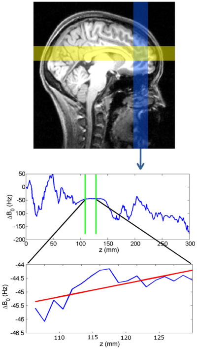
Top: 2-dimensional RF pulses sequentially excite three spatial columns, two of which are shown in yellow and blue on a sagittal brain cross section (the third column is perpendicular to the page). Two gradient echoes are acquired for each column. Center: a phase difference map for the inferior-to-superior column, from which the B₀ field distribution is calculated (averaged across the column cross-section). The values that fall inside the VOI (between green lines) are selected for further processing. Bottom: A linear fit is performed on ΔB₀ values within the VOI (red line). The slope of this line provides one of the 3 components of the desired correction gradient.

Following each 2D excitation pulse, two frequency-encoded gradient echoes were acquired (TE₁=6.97ms and TE₂=20.77ms), using 256 readout points with a bandwidth of 78Hz/pixel. The readout was in the direction of the long column axis. Since the 2D excitation generated signal only from the column, a 1D readout is sufficient to measure the localized field distribution across the voxel. The field map from each of the 3 columns represents the B₀ strength along the column axis, averaged across the column cross section. For the parameters used in this study, the field map voxels are 20×20×1.17mm³≈470μL. The large size of the voxels assures abundant SNR and justifies the use of a small flip angle. The entire B₀ mapping module takes approximately 120ms to acquire.

Reconstruction of the B₀ field distribution consisted of 1D fast Fourier transformation, computation of the complex ratio between the two echoes and phase unwrapping. Field map pixels that fall within the MRS VOI were identified and linear fits were performed to determine the optimal correction gradient. These computations were performed in real-time and the resulting shim corrections were sent back to the sequence where the linear shims were updated for subsequent PRESS acquisitions.

Frequency Updates

Frequency changes are caused both directly by head motion and indirectly by the applied shim corrections. Although retrospective frequency corrections may be performed on individual free induction decays (FID’s), real-time frequency updates are necessary to ensure accurate 2D excitations (which are sensitive to off-resonance), effective water suppression and accurate voxel position. Therefore, immediately after each PRESS acquisition, the position of the residual water peak in each FID was identified and any motion-induced frequency shift was subtracted from the center frequency. Additionally, dynamic shim-induced frequency shifts at the center of each VOI were computed and corrected for at the same time. Frequency correction was implemented by updating the center frequency for all radio frequency (RF) pulses and analog-to-digital converter (ADC) events in the sequence. Frequency updates and dynamic shimming were performed during dummy acquisitions as well as during acquired FID’s.

Retrospective Frequency and Phase Corrections

A cycled water suppression scheme was employed in our experiments to enable retrospective frequency and phase corrections, while ensuring an undistorted spectral baseline (4). This weak water suppression/phase cycling module was [played out] immediately prior to the PRESS excitation and has a similar duration as the conventional water suppression module (approximately 200ms).

Experiments

Our dynamic shimming / frequency adjust system was validated both in phantom and in vivo studies. All experiments were performed on a Siemens Tim Trio 3T full-body scanner (software version VB17) with a 12-channel phased array head coil. Phantom experiments were performed on a spherical spectroscopy phantom. Informed consent was obtained from 8 human subjects, in compliance with the local Institutional Review Boards. Prior to the start of each scan, a voxel was placed in the desired location (magnet isocenter for phantom scans, frontal gray matter in vivo). The second-order shims were set to the so-called “tune-up” values (appropriate for imaging) in order to ensure relatively distortion-free navigator images, and the linear shims were manually optimized for the MRS VOI. Typical metabolite line widths at the start of the scans were ≤0.015ppm (2Hz) in the phantom and ≤0.06ppm (7.5Hz) in vivo.

In the first phantom experiment, the linear shims were offset by a known amount from the optimal values prior to the start of the scan. Specifically, the shim setting was changed in each of the three coordinate directions by −15 to +15μT/m in 5μT/m increments. The linear corrections calculated by the dynamic shimming module were then compared to these known offsets. In the second phantom experiment, a large water bottle was placed in close proximity to the phantom during the scan in order to induce unknown (linear and/or higher order) changes in B₀. This procedure was performed twice, with and without frequency/shim corrections. Since the MRS phantom used in these experiments was spherical and lacked internal structure, PROMO does not perform correctly, and motion correction was turned off during all phantom experiments.

For the in vivo experiments, the voxel was placed in the medial frontal lobe (Fig. 2). Four spectra were collected from each subject: 1. a baseline (BL), in which the subject remained still and no real-time corrections were applied, 2. a corrected-baseline scan, in which the subject was again still, but with real-time motion- and shim-corrections turned on, 3. an uncorrected motion scan, in which the subject moved, motion correction was turned on, but shim and frequency corrections were off, and 4. a corrected motion scan in which the subject moved and both motion- and shim/frequency corrections were turned on. Note that motion correction (PROMO) was employed for all scans except for the BL, and that “corrected” and “uncorrected” refer to dynamic shimming and frequency updates in the current paper.

Prior to the scan, subjects were trained to perform an x-rotation (chin down-to-up) of 10–20° on cue. This type of motion induces B₀-field changes (11) and is a natural and common motion in the scanner environment. All subjects were instructed to perform the designated movement at a moderate rate (a few degrees per TR) typically starting at the 2^nd or 3^rd average, and to remain in the new position until the scan was complete. Therefore, most of the averages were acquired during or after movement, maximizing the effects of motion on the final spectrum. After each MRS scan, subjects returned their heads to the initial position and the voxel placement was checked and corrected (if necessary) via a quick localizer scan before obtaining further spectra. We report the motion amplitudes as the vector magnitudes ||t_x, t_y, t_z)|| and ||(θ_x, θ_y, θ_z)||, where t_i are the translations in mm and θ_i are the Euler angles in degrees of the head pose at the end of each scan relative to the start of the scan.

All 32 individual FIDs were saved separately. Following Fourier transformation, individual raw spectra were frequency- and phase corrected, and averaged using a custom Matlab (The MathWorks, Natick, MA) program before being quantified with LCModel (17). Signal-to-noise ratio (SNR) and the full-width at half-maximum (FWHM) of spectral peaks as determined by LCModel were used as the primary indicators of overall spectral and shim quality. The effects of dynamic shimming on metabolite measurements were assessed by comparing the measured metabolite ratios of the BL spectrum to the ratios from the other three acquisitions using paired t-tests with the Bonferroni correction for multiple comparisons. Metabolite levels were expressed relative to total creatine (Cr), and included N-acetylaspartate (NAA/Cr), total choline (Cho/Cr), glutamate + glutamine (Glx/Cr) and myo-inositol (mI/Cr). Additionally, one experienced researcher (T.E.) who was blinded to the scan conditions rated each spectrum qualitatively as “excellent”, “good”, “acceptable” or “bad.” A “bad” rating indicated that the data was deemed unusable, and would be rejected in a standard QA procedure. Since the ratings are ordinal variables, they were compared statistically using the non-parametric Wilcoxon rank sum test.

RESULTS

Phantom Experiments

In the first phantom experiment, there was excellent agreement between the measured shim corrections and applied shim offsets. Since a small error is expected for manual shimming, each of the 3 components was fitted to a linear function with an offset. After adjusting for the imperfect manual shim (constant shim offset), the dynamic shim module detected linear B₀ variations almost perfectly in the phantom, with a mean error magnitude of 0.003±0.21uT/m across all averages and all scans. A linear regression on all components yielded a slope of 1.0029 (R²=0.9996).

Figure 3 shows the phantom spectra acquired when a water bottle was moved close to the phantom during the scan. The line widths of the uncorrected and corrected spectra were 0.052ppm and 0.014ppm, respectively, as compared to BL line widths of 0.010ppm (not shown). The SNR of the BL spectrum was 52, the SNR of the uncorrected spectrum was 7 and the frequency/shim correction restored the SNR to 50. The line broadening displayed by the uncorrected spectrum affected the metabolite measurements, since the measured concentrations ratios from the corrected spectrum agreed with the BL values better than those of the uncorrected spectrum for all major metabolites. The improvement in the corrected spectrum compared to the uncorrected one is due not only to the application of dynamic shim corrections, but also the update of the water suppression frequency. The frequency change for the uncorrected scan was 33Hz, which was sufficient to cause ineffective water suppression, and interfered with the water suppression cycling algorithm.

FIG. 3.

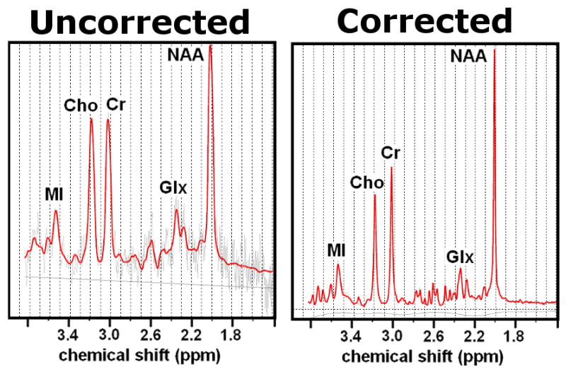
Uncorrected (left) and corrected (right) spectra acquired from the phantom with an adjacent water bottle. In the uncorrected spectrum, sub-optimal shim and poor water suppression result in increased line widths, reduced SNR and an elevated baseline.

In Vivo Experiments

Representative motion trajectories and corresponding spectra for one subject are shown in Figure 4. All 8 subjects were largely successful in remaining motionless during the corrected-baseline scan, with measured translations <0.5mm and rotations <0.5° in all directions for all subjects. During the motion scans, subjects performed the motion correctly but then involuntarily moved partially back towards the initial position, presumably due to fatigue. This can be seen most clearly in the trajectory of the uncorrected scan in Fig. 4. Steady-state motion amplitudes, as measured by the head pose at time of the final MRS average, were (4.7±2.9mm, 12.8±6.0°) for the uncorrected scans and (5.4±3.7mm, 13.7±5.9°) for the corrected scans, a statistically non-significant difference. These movements were executed over 3–5 TR periods (10–15 sec). All subjects were able to reproduce the same motion trajectories for the uncorrected- and corrected-motion scans to within approximately 4mm and 5°.

FIG. 4.

Top row: four spectra acquired from a single subject under various scan conditions. The uncorrected spectrum has poorer line width and reduced SNR compared to the other 3 spectra. See text for details. Bottom row: rigid-body motion trajectories during data acquisition, with blue = x-component, green = y-component and red = z-component. Prospective motion correction was applied for all scans except baseline.

All in vivo shim-corrected scans demonstrated an initial shim offset of unknown origin, even in the absence of motion (average magnitude 11.3±6.1μT/m). After subtracting the initial gradient offset, the applied correction gradients during the corrected-BL were 1.1±0.3μT/m in magnitude. In the presence of motion, the shim correction gradients were highly variable across subjects, even for similar motion trajectories. Correction gradients for the motion scans, both corrected and uncorrected, were 12.8±4.8μT/m in magnitude during the final average (corresponding to a line width of approximately 0.09ppm across the 20mm voxel) and ranged from 5.2μT/m to 21.0μT/m.

The line widths and SNR for all subjects’ scans are shown in Figure 5. The average line widths were 0.044±0.008ppm, 0.057±0.006ppm, 0.067±0.03ppm and 0.048±0.014ppm for the BL, corrected-BL, uncorrected and corrected scans, respectively (mean±standard deviation). Importantly, the line widths of corrected spectra were significantly better than those of the uncorrected spectra (p=0.013, paired t-test), even though the average motion was larger during the corrected scans. The metabolite ratios measured during the corrected-BL, uncorrected and corrected scans did not differ significantly from the BL in paired t-tests after correcting for multiple comparisons.

FIG. 5.

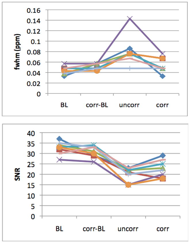
The line widths at full width half maximum (FWHM) (top) and signal-to-noise ratio (SNR) (bottom) of each subject’s scans for the 4 different scan conditions. Abbreviations: BL = baseline; corr-BL = baseline scan with corrections on; uncorr = scan with motion but no correction; corr = scan with motion and correction on.

In the scans with motion, the corrected spectrum had narrower peaks and higher SNR than the corresponding uncorrected spectrum in every subject. In 5 subjects, the corrected line widths agreed with the BL to within 0.01ppm, whereas the corrected line widths were broader than those of the corresponding BL in the remaining 3 subjects. Consequently, the average line widths of the corrected scans were only minimally larger compared to those of the BL scans (BL=0.044ppm vs. corrected-BL=0.048ppm). Interestingly, in one subject, a motion of (4.9mm, 10.7°) had little effect FWHM of the spectra (flat line in Fig. 5); all four of this subject’s spectra had similar line widths and were qualitatively similar. Similarly, the SNR of the corrected spectrum was better than that of the uncorrected spectrum but slightly worse than that of the BL in all subjects.

The blinded ratings generally tracked the line widths, with spectra displaying narrow line widths receiving favorable ratings. In every subject, uncorrected spectra were rated worse than the corresponding BL’s, and corrected spectra were rated better than uncorrected spectra. The uncorrected spectra were rated significantly worse (0.028<p<0.018, Wilcoxon signed-rank tests) than the other three spectra. No other pairs of ratings were statistically different.

DISCUSSION

We have developed a novel method to characterize linear B₀ variations over a small volume of interest in as little as 100ms using two-dimensional RF excitations. The method was implemented for dynamic shimming in localized spectroscopy scans, in conjunction with real-time prospective adjustment of center frequency. Together, these two techniques significantly improved spectral line widths and SNR during subject motion. While dynamic shim/frequency correction did not substantially improve the reproducibility of measured metabolite concentrations in our small pilot study, narrower line widths are generally associated with better spectral quantification (10). Future work will include testing the sequence in a larger population to verify that intra- and inter-subject metabolite variability is reduced as compared to a standard PRESS acquisition. Although these techniques were implemented for single-voxel brain MRS, the principles may be adapted for MRS of other body parts or spectroscopic imaging (SI).

In our experience, the quality of the shim corrections is rather insensitive to the exact scan parameters (bandwidth, flip angle, resolution), most likely due to the relatively large volume of field map voxels (approximately 0.5cc), which provide abundant SNR. The specific acquisition parameters used for the current study resulted in an acquisition time of ~120ms, including reconstruction, to measure the linear variation of B₀ in all three coordinate directions. This time could be considerably reduced if the host sequence requires it, possibly at the expense of SNR and/or quality of the 2D profile.

Our dynamic shimming method represents a marked improvement over performing no correction when the amplitude of subject motion is quite large, as was the case in our experiments. However, in the absence of motion, corrections slightly increased line widths (corrected-BL in Fig. 5). This increase in line widths is consistent with the small, but non-zero, shim corrections applied during the corrected-baseline. The robustness of the shim corrections might be improved with a different selection of parameters or by restricting fitting of the field map to the center of the VOI. Alternatively, one could update the shim only when the motion magnitude exceeds a predefined threshold. The quality of the final spectrum might also be improved by rejecting individual FID’s from the final summation when the estimated velocity (i.e., difference between consecutive head poses) is large.

In this study, dynamic shimming was accomplished using first-order shim corrections only. Higher-order (>1) shims cannot be changed in real time on most commercial scanners, since standard shim coils are not designed for rapid switching, and inadequate shielding results in large, slowly decaying eddy currents (18). The use of first-order gradient corrections is likely to be sufficient in the case of single-voxel spectroscopy, where the region of interest is small enough (~2cm) that linear shims are able to achieve line widths of ≤0.05ppm in most cases. Thus, for sufficiently small VOIs, effective dynamic shimming is possible without additional hardware.

The field mapping method described here is a case of projection-based shimming (19), since it involves averaging signals and phases over a relatively large cross section (the MRS voxel). A careful analysis reveals that non-linear phase variations in one direction can influence the projection-based measure of linear variation in orthogonal directions (20); for instance, a large z² dependence in B₀ may alter the projection-based measure of x and y shims. However, these effects are most likely small in the current study since the relevant volume is only 20mm across, so higher-order field terms are unlikely to show much effect. If our method were to be used to shim a larger VOI, for instance an entire slice for chemical shift imaging (as in (8)), then the effects of such “cross-talk” may need to be accounted for.

Hess and colleagues recently presented an alternative method for achieving simultaneous motion- and shim-correction in single voxel MRS using 3D echo-planar imaging (EPI) navigators (6). Field maps were computed for the entire navigator volume by acquiring navigator images twice with different TE’s. The relative advantages of the present method are 1) shorter acquisition time (approximately 120ms vs. 550ms), 2) simple and fast phase unwrapping (1D vs 3D), and 3) separating field mapping from motion correction, i.e., our dynamic shimming method is easy to implement in conjunction with non-MR based tracking systems, such as optical tracking (9,21).

The use of 1D readouts means that we are averaging the signal in planes across the entire imaged object, and are relying on the 2D excitations for localization. Due to the short duration of the 2D excitations, non-negligible amounts of signal were excited away from the VOI. In addition, the efficacy of the 2D pulses relies on an accurate frequency adjustment, and on the quality of the initial shim. Any signal that is excited outside the VOI will be averaged into the field maps, and introduce errors in the B₀ measurement. Such unwanted signals may be responsible for the differences in accuracy between phantom and in vivo experiments, as well as the shim offsets that were evident for in vivo B₀ measurements, since off-resonance effects, higher-order B₀ variations and flow effects are all expected to be more significant in vivo. More sophisticated RF pulse design might yield a more accurate excitation profile with better immunity to off-resonance effects, and is the focus of ongoing work.

SUMMARY

Localized MRS sequences are ideal candidates for incorporating real-time motion correction due to the large amounts of unused scan time. Accordingly, we have been able to develop a comprehensive, motion-insensitive PRESS sequence that combines adaptive motion correction with dynamic shimming, real-time frequency correction, and a water suppression cycling scheme to enable frequency and phase correction of individual FIDs.

References

- 1.Felblinger J, Kreis R, Boesch C. Effects of physiologic motion of the human brain upon quantitative 1H-MRS: analysis and correction by retro-gating. NMR Biomed. 1998;11(3):107–114. doi: 10.1002/(sici)1099-1492(199805)11:3<107::aid-nbm525>3.0.co;2-i. [DOI] [PubMed] [Google Scholar]
- 2.Helms GPA. Restoration of motion-related signal loss and line-shape deterioration of proton MR spectra using the residual water as an intrinsic reference. Magn Reson Med. 2001;46:395–400. doi: 10.1002/mrm.1203. [DOI] [PubMed] [Google Scholar]
- 3.Star-Lack JM, Adalsteinsson E, Gold GE, Ikeda DM, Spielman DM. Motion correction and lipid suppression for 1H magnetic resonance spectroscopy. Magn Reson Med. 2000;43(3):325–330. doi: 10.1002/(sici)1522-2594(200003)43:3<325::aid-mrm1>3.0.co;2-8. [DOI] [PubMed] [Google Scholar]
- 4.Ernst T, Li J. A novel phase and frequency navigator for proton magnetic resonance spectroscopy using water-suppression cycling. Magn Reson Med. 2011;65(1):13–17. doi: 10.1002/mrm.22582. [DOI] [PMC free article] [PubMed] [Google Scholar]
- 5.Keating B, Deng W, Roddey JC, White N, Dale A, Stenger VA, Ernst T. Prospective motion correction for single-voxel 1H MR spectroscopy. Magn Reson Med. 2010;64(3):672–679. doi: 10.1002/mrm.22448. [DOI] [PMC free article] [PubMed] [Google Scholar]
- 6.Hess AT, Dylan Tisdall M, Andronesi OC, Meintjes EM, van der Kouwe AJW. Real-time motion and B0 corrected single voxel spectroscopy using volumetric navigators. Magn Reson Med. 2011;66(2):314–323. doi: 10.1002/mrm.22805. [DOI] [PMC free article] [PubMed] [Google Scholar]
- 7.Zaitsev M, Speck O, Hennig J, Buchert M. Single-voxel MRS with prospective motion correction and retrospective frequency correction. NMR Biomed. 2010;23(3):325–332. doi: 10.1002/nbm.1469. [DOI] [PubMed] [Google Scholar]
- 8.Lange T, Maclaren J, Buechert M, Zaitsev M. Spectroscopic imaging with prospective motion correction and retrospective phase correction. Magnetic Resonance in Medicine. 2011 doi: 10.1002/mrm.23136. [DOI] [PMC free article] [PubMed] [Google Scholar]
- 9.Andrews-Shigaki BC, Armstrong BS, Zaitsev M, Ernst T. Prospective motion correction for magnetic resonance spectroscopy using single camera Retro-Grate reflector optical tracking. J Magn Reson Imaging. 2011;33(2):498–504. doi: 10.1002/jmri.22467. [DOI] [PMC free article] [PubMed] [Google Scholar]
- 10.de Graaf RA. In Vivo NMR Spectroscopy. West Sussex, England: John Wiley & Sons; 2007. [Google Scholar]
- 11.Keating B, Ernst T. Motion-Induced Frequency and Shim Variations During Localized 1H MR Spectroscopy with Prospective Motion Correction. Stockholm, Sweden: 2010. [Google Scholar]
- 12.Boegle R, Maclaren J, Zaitsev M. Combining prospective motion correction and distortion correction for EPI: towards a comprehensive correction of motion and susceptibility-induced artifacts. MAGMA. 2010;23(4):263–273. doi: 10.1007/s10334-010-0225-8. [DOI] [PubMed] [Google Scholar]
- 13.Bottomley P. Spatial localization in NMR spectroscopy in vivo. Ann NY Acad Sci. 1987;508:333–348. doi: 10.1111/j.1749-6632.1987.tb32915.x. [DOI] [PubMed] [Google Scholar]
- 14.White N, Roddey C, Shankaranarayanan A, Han E, Rettmann D, Santos J, Kuperman J, Dale A. PROMO: Real-time prospective motion correction in MRI using image-based tracking. Magn Reson Med. 2010;63(1):91–105. doi: 10.1002/mrm.22176. [DOI] [PMC free article] [PubMed] [Google Scholar]
- 15.Cline HEZX, Gai N, Gai Design of a Logarithmic k-Space Spiral Trajectory. Magn Reson Med. 2001;46:1130–1135. doi: 10.1002/mrm.1309. [DOI] [PubMed] [Google Scholar]
- 16.Traber F, Block W, Lamerichs R, Gieseke J, Schild HH. 1H metabolite relaxation times at 3. 0 tesla: Measurements of T1 and T2 values in normal brain and determination of regional differences in transverse relaxation. J Magn Reson Imaging. 2004;19(5):537–545. doi: 10.1002/jmri.20053. [DOI] [PubMed] [Google Scholar]
- 17.Provencher SW. Automatic quantitation of localized in vivo 1H spectra with LCModel. NMR Biomed. 2001;14(4):260–264. doi: 10.1002/nbm.698. [DOI] [PubMed] [Google Scholar]
- 18.de Graaf RA, Brown PB, McIntyre S, Rothman DL, Nixon TW. Dynamic shim updating (DSU) for multislice signal acquisition. Magn Reson Med. 2003;49(3):409–416. doi: 10.1002/mrm.10404. [DOI] [PubMed] [Google Scholar]
- 19.Ward HA, Riederer SJ, Jack CR. Real-time autoshimming for echo planar timecourse imaging. Magn Reson Med. 2002;48(5):771–780. doi: 10.1002/mrm.10259. [DOI] [PubMed] [Google Scholar]
- 20.Splitthoff D, Zaitsev M. Theoretical Basis of Projection Based Shimming. Montreal, Quebec: 2011. [Google Scholar]
- 21.Zaitsev M, Dold C, Sakas G, Hennig J, Speck O. Magnetic resonance imaging of freely moving objects: prospective real-time motion correction using an external optical motion tracking system. NeuroImage. 2006;31(3):1038–1050. doi: 10.1016/j.neuroimage.2006.01.039. [DOI] [PubMed] [Google Scholar]