Identification and evaluation of cycling yeast metabolites in two-dimensional comprehensive gas chromatography–time-of-flight mass spectrometry data

Abstract

A yeast metabolome exhibiting oscillatory behavior was analyzed using comprehensive two-dimensional gas chromatography - time-of-flight mass spectrometry (GC × GC–TOF-MS) and in-house developed data analysis software methodology, referred to as a signal ratio method (Sratio method). In this study 44 identified unique metabolites were found to exhibit cycling, with a depth-of-modulation amplitude greater than three. After the initial locations are found using the Sratio software, and identified preliminarily using ChromaTOF software, the refined mass spectra and peak volumes were subsequently obtained using parallel factor analysis (PARAFAC). The peak volumes provided by PARAFAC deconvolution provide a measurement of the cycling depth-of-modulation amplitude that is more accurate than the initial Sratio information (which serves as a rapid screening procedure to find the cycling metabolites while excluding peaks that do not cycle). The Sratio reported is a rapid method to determine the depth-of-modulation while not constraining the search to specific cycling frequencies. The phase delay of the cycling metabolites ranged widely in relation to the oxygen consumption cycling pattern.

1. Introduction

Comprehensive two-dimensional gas chromatography (GC × GC) is a very powerful technique based on the separation of gas phase analytes on two capillary columns, i.e., column 1 and 2, with complementary interactions [1]. A modulation device collects the column 1 effluent and then rapidly injects narrow pulses onto column 2 [2-5]. The peak capacity of the two-dimensional (2D) separation system is multiplicative and results in an increase in the number of compounds the system can separate, over one-dimensional (1D) GC [6]. The coupling of the GC × GC instrument to a univariate detector such a flame ionization detection (FID) system often yields informative structured 2D chromatograms, with compounds in the same class along diagonal lines [7-9]. Coupling the GC × GC to a multivariate detector, such as a mass spectrometer (MS), yields an increase in information over a GC × GC-FID instrument, thus making the GC × GC-MS more ideal to study complex samples. GC × GC-MS instrumentation provides a third dimension of data that allows the analyst to more readily distinguish compounds. In addition to the class information output by the 2D GC × GC-FID chromatograms, GC × GC-MS instrumentation can generate a full mass spectrum for each analyte peak thus providing significant insight for the identification of compounds.

Recently, the advent of commercially available time-of-flight mass spectrometry (TOF-MS) systems interfaced to GC × GC systems led to the broadening use of the third order GC × GC-MS instrumentation [10,11] (column 1, column 2, and full mass spectrum) and has been applied to the study of metabolomic samples [12-18]. Metabolomic samples are sufficiently complex for analysis on a third order instrument for example, with ~ 200 000 different metabolites in the plant kingdom [19,20] and ~ 600 metabolites in yeast [21,22]. A limiting factor in the analysis of metabolomic data is the high dimensionality and complexity of the data [23-26]. In order to make biological conclusions concerning the data, some form of data reduction, i.e., chemometrics (or bioinformatics), must be applied to the data to rapidly locate and sort the metabolites in order of biological importance. Metabolites are found in a wide range of concentrations, with the most concentrated metabolites not always being the most important nor informative [27]. Following identification of important metabolites, the metabolites must be accurately quantified. In order to save on the overall analysis time, the above mentioned data analysis steps should ideally be compiled into high-throughput discovery-based software that is also user friendly [28,29]. Indeed, there is an on-going need to develop improved chemometric tools that can readily be applied to third order GC × GC–TOF-MS metabolomics data in a discovery-based manner.

The first step in data analysis is to locate peaks in the 2D separation space that are changing between sample types. One method to objectively locate peaks is the use of principal component analysis (PCA) [12,30]. PCA is an unsupervised method that does not require class specification. Hence, application of PCA does not necessarily take advantage of the experimental design knowledge and is, therefore, also subject to problems due to within-class variation. Each sample is compared with all other samples to determine where the greatest variation in signal intensity lies. Those regions of the chromatograms with the greatest variation between samples are captured on the first principal component (PC1), with each decreasing principal component describing less variance. Every sample is assigned a score value on each PC and each variable (chromatographic peak) is assigned a loading value. The samples with similar scores show less variation in signal intensities. A second chemometric data reduction tool recently reported for use with GC × GC–TOF-MS metabolomics data is based on Fisher ratios [14,31]. The Fisher ratio method, unlike PCA, is intrinsically a supervised method making it a more ideal method for analysis of samples generated via hypothesis driven research, where the origin of samples, and thus the class membership, is known. Since the Fisher ratio is the average class-to-class variation divided by the within-class variation, multiple samples from each sample type must be collected and the class of each sample specified. Some benefits to using the Fisher ratio method over PCA are that the Fisher ratio method has been automated to analyze the entire three-dimensional (3D) data output by the third order instrumentation and the Fisher method considers each point in the 2D separation space independently, making it more robust than PCA to within-class variation. One major drawback to both of these methods is that as the number of sample classes increases, the ability to find metabolites that are distinguished by class becomes more difficult, if not impossible if there are too many sample classes. This drawback is addressed in the report herein.

Following data reduction to find the locations in the 2D separation space that contain class distinguishing metabolites, these locations must be “mined” to positively identify and quantify the metabolites. Although the 2D separation space provides a large peak capacity, some peaks might overlap (co-elute) in one of the separation dimensions. To address this issue, a parallel factors analysis (PARAFAC) graphical user interface (GUI) was developed to mathematically resolve 3D data by comparison to a target analyte specified by the user [32,33]. Prior to target analysis using PARAFAC, an initial identification of the analyte must be specified. The ChromaTOF software is used to provide the initial analyte identification for the PARAFAC GUI for the 2D locations being mined. The outputs of this PARAFAC GUI are pure column 1, column 2 and mass spectral profiles, which can then be transformed into a 3D peak to obtain accurate peak volume information. Given sufficient selectivity across the three dimensions, PARAFAC has been shown to yield accurate identification and quantitative information for GC × GC–TOF-MS data [13]. Automation of this PARAFAC GUI to analyze multiple analytes has greatly reduced the overall analysis time of the complete data set. Comparison of the PARAFAC deconvoluted mass spectrum to library spectra and the initial spectrum provided by ChromaTOF provides considerable confidence in analyte identification.

Within the last few years, two groups have reported yeast cells exhibiting periodicity in genome-wide transcription, as a function of robust oscillations in oxygen consumption that occur under continuous, steady-state growth conditions [34,35]. The McKnight group reported an ultradian yeast metabolic cycle (YMC) of about four to five hours in length [34], while Klevecz and co-workers reported cycles lasting around 40 minutes in length [35]. An illustration of the oscillating dO₂ as observed by the McKnight group is shown in Figure 1 with the locations of sample collection time intervals marked with dots (as explained in more detail in the Experimental section). Twelve time intervals were collected over each of the two 5 hour cycles with each interval separated by 25 minutes. Upon analysis of the periodic gene expression profiles, we hypothesize that many cellular metabolites would exhibit periodic oscillations in cellular concentration.

Figure 1.

Illustration of dissolved oxygen content (dO₂) and a hypothetical metabolite trace in yeast grown under continuous nutrient limited conditions is shown, with one cycle lasting 5 h. Samples were collected every 25 min as shown by the dots on the dO₂ trace. The locations of the time intervals averaged for Smax and Smin are shown by the “x” on the predicted metabolite trace per Eq. 1.

Reported herein is a method for analyzing three-way GC × GC–TOF-MS data of 24 sample aliquots (i.e., time intervals) from yeast cells grown under continuous, nutrient-limited conditions. Due to the large number of time intervals collected and the similar concentrations of metabolites in adjacent time intervals, PCA and Fisher analysis were not effective data reduction methods for this study. Since it was hypothesized that the samples would show periodic behavior, a data analysis method was developed that measures the amplitude (depth of modulation) of the periodic pattern based on the strongest and weakest signal intensities for each metabolite, and has been termed the Sratio method. Because it was the depth of modulation that was determined, no frequency constraints were placed on the data, thus allowing metabolites with higher or lower frequencies than that of the dO₂ shown in Figure 1 to be located. Also the depth of modulation is independent of signal intensity. Even though the depth of modulation was calculated for each metabolite over all m/z, thus utilizing all mass channel information, only the three most selective m/z for a given metabolite were ultimately used to obtain the locations of those metabolites in the 2D separation space showing periodic patterns. Following this data reduction to find the locations of cycling metabolites, and initial mass spectral identification using ChromaTOF, the PARAFAC GUI was applied to provide a refined deconvoluted mass spectrum and to determine a more accurate depth of modulation based on the deconvoluted 3D peak volumes (Vratio information). Metabolites that show similar patterns were then determined by submitting the Vratios to PCA to better understand the cycling patterns observed. The method we report is significantly different from the Fourier Transform based method Murray and co-workers reported earlier this year when analyzing samples using GC-MS instrumentation [36]. Their method was set to locate metabolites cycling at the same frequency as the dO₂ and did not take the discovery-based approach we report, i.e., find locations of all cycling metabolites regardless of frequency. Murray et. al. also reported a very rapid temperature program (30°/min) for their GC–TOF-MS method. This temperature program rate led to large overlap of chromatographic peaks and there is no indication in the report as to the confidence of the metabolite identification, e.g., mass spectral match values, retention time confirmation was not provided. Herein, we provide confident metabolite identification.

2. Theory

The yeast metabolites analyzed in this study were predicted to express a periodic cycling of concentration levels during the metabolic cycles, similar to the pattern seen in the dO₂ signal, Figure 1. Previously, oscillations in the mRNA levels of many genes encoding metabolic enzymes with this periodicity were observed. After the concentration of dO₂ in the culture medium was cycling, samples of the continuous culture were taken at regular time intervals and submitted to GC×GC–TOF-MS analysis. Each sample analysis was performed in triplicate. This produced a five-dimensional array where the dimensions were retention time on column 1, retention time on column 2, m/z, time interval (i..e., sample number), and replicate number. Since 24 time intervals were collected for this study (constituting 24 sample classes), the use of PCA and the Fisher ratio method failed to locate many of the differentiating locations (i.e., cycling metabolites) in the 2D separation space. The data processing method developed for this study uses the ratio of chromatographic signals at each mass channel (m/z) between samples to find the locations in the 2D separation space that contain cycling metabolites and is, therefore, named the Sratio method.

The Sratio method, illustrated in Figure 2, determines the magnitude of changes in metabolite signal intensities during cycling using the most selective m/z in an automated and objective fashion. For each m/z, the data for each sample number were removed from the original five-dimensional array and compiled into a new single m/z four-dimensional array, where the four dimensions are retention time on column 1, retention time on column 2, sample number and replicate number. Each of these arrays, at a given m/z, was then unfolded for 1D alignment along retention time on column 2. The narrowness of peaks from column 2 (50-100 ms width at peak base) caused the observed retention shifting on column 2 to have a more detrimental impact on the Sratio calculation than shifting on column 1, if left uncorrected prior to taking the Sratio. A majority of the run-to-run retention time shifting on column 1 was approximately one-half a modulation period and resulted from being either in phase or out of phase with the modulation, whereas the shifting on column 2 ranged from -30 to +30 ms. It was predicted using a Gaussian peak concentration model for column 2 that for a peak shifted 20 ms with a width at the base of 100 ms a 37% decrease in signal intensity would be observed and for the same shifting of a 70 ms wide peak a 48% decrease in signal intensity would arise. Peaks shifted by a half a modulation period on column 1 were predicted to only have a 12% decrease in signal intensity, in relation to the peak widths on column 1. Thus, retention time alignment on column 1 was deemed unnecessary, because the error invoked by ignoring shifting on column 1 was much less than the time interval-to-time interval biological variation, which was ~30% RSD. Thus, if signal intensity ratios (Sratios as defined below) were calculated at a specific point in the 2D separation space, retention misalignment would cause inflated ratios, much more so on column 2, hence alignment was applied on column 2 only to overcome this issue. The aligned chromatograms, at a given m/z, were then refolded and augmented back into four-dimensional arrays. These aligned four-dimensional arrays were summed simultaneously along the sample number and replicate number dimensions to produce a summed 2D separation matrix. In this summed 2D separation matrix local peak maxima were found by testing each element of the matrix to determine if it was a local maximum having a value above a calculated noise threshold value, which, if both conditions were true, indicated that there was an observed peak maximum at the corresponding point in 2D separation space. The locations of the peak maxima were retained in the aligned data for each sample (across the replicates), and the remaining chromatographic locations in the 2D separation space zeroed. The data were then averaged along the replicate dimension so that there was only a 2D array for each time interval (sample number) at a given m/z. Since data were collected over two metabolic cycles, the algorithm found the samples with the two greatest chromatographic signals at each 2D retention time, i.e., at each peak maxima, in the 2D separation space and calculated an average, Smax. The samples with the two lowest signals at each peak maxima were also found and the average calculated, Smin. An illustration, at a given m/z, of the samples averaged for Smax and Smin are depicted by the “x’s” in the hypothetical metabolite trace in Figure 1. If the Smax or Smin was lower than the user specified noise threshold, the value at that point was replaced with a user-selected noise threshold value. The Sratio was then calculated, as the ratio of the maximum and minimum raw chromatographic signals at each 2D peak maxima location:

$$S_{\mathit{ratio},X}=\frac{S_{\max ,X}}{S_{\min ,X}},\mathrm{at}m/z\mathrm{X}$$ (1)

and returns the average signal amplitude, i.e., depth of modulation, of the cycling pattern for each peak maxima in the 2D separation space for each m/z. Chromatographic locations with larger Sratios have a greater change in signal during cell growth and thus pinpoint the 2D chromatographic locations to study in greater detail. These steps were then repeated for all m/z to obtain a Sratio “mass” spectrum for each peak maxima in the chromatographic space. The n largest Sratios across all m/z were averaged to give an overall Sratio at each retention time point, and for each m/z, in the 2D separation space:

$$\overline{S}\mathit{ratio}=\frac{\sum _{i=1}^n(S_{\mathit{ratio},i})}{n}$$ (2)

Figure 2.

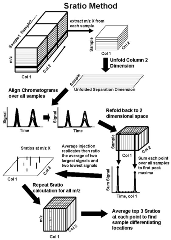
A stepwise schematic explaining the Sratio method, which extracts only the most selective information to determine the sample differences. One mass channel, m/z, is removed from each sample (per replicate) and compiled into one data cube. Each sample (per replicate) is unfolded to remove the second dimension and aligned to the first sample. The samples, for given replicate, are then refolded back into the data cube and each point in the 2D separation space summed over all samples to pinpoint peak maxima. The injection replicates are then averaged. The peak heights from the two samples with the largest signals at each point in the chromatographic space are averaged, providing Smax. The two lowest signals over all samples at each point were also averaged, providing Smin. A ratio of Smax to Smin was then calculated at each m/z to give insight into the amplitude of the cycles for each peak. This process is then repeated in an automated fashion over all m/z specified to obtain a Sratio spectrum at each point in the 2D chromatographic space. The three largest Sratios are averaged to find chromatographic locations that contain cycling metabolites.

For the results reported herein, n was equal to three. This average of the three most intense Sratios disposes of noise, some reagent artifacts and peaks arising from peak maxima misaligned in one or two m/z. The average of three or more Sratios also minimizes the bias from overlapping interferents at the less selective m/z. An RSD (standard deviation of “n” largest Sratios/average of “n” largest Sratios) threshold can also be specified for the average Sratio per Equation 2 to remove artifacts with more than three Sratio values, but in which the Sratios vary too wildly in intensity. Peaks arising from metabolites tend to have less variation in the Sratio intensities. Specific parameters used in this study will be described in the Data Analysis section.

3. Experimental

3.1 Cell growth, extraction and derivatization

Yeast manipulations and continuous culture experiments using the diploid yeast strain CEN.PK were performed as previously described [34]. Dissolved oxygen levels were monitored every 30 s continuously using a Metter Ingold InPro 6800 in-line dissolved oxygen sensor (Mettler-Toledo Ingold, Bedford, MA, USA). The quenching of metabolic activity and extraction of intracellular metabolites was performed using a method adapted from Castrillo et. al. [37]. Following growth to high density (OD~8-9), 1 ml of the continuous chemostat culture was rapidly quenched (4 ml 10 mM tricine, pH 7.4, 60% methanol) at -40 °C, for each time interval. Cells were spun at 1 000 g for three minutes at -10 °C, washed with 1 ml of the quenching buffer, and resuspended in 1 ml of extraction buffer (0.5 mM Tricine, pH 7.4, 75% ethanol) at 80 °C for three minutes followed by incubation at 4 °C for five minutes. Samples were spun at 20 000 g to remove cell debris and stored at -80 °C until analysis. Twenty-four samples, each containing ~1 × 10⁸ cells were collected every 25 min for 10 h resulting in 24 time intervals. Metabolites were derivatized following the protocol described previously using methoximation (20 mg/ml methoxyamine in pyridine) and trimethylsilylation (BSTFA:TMCS, 99:1) [12].

3.2 Instrumentation

Three-way GC × GC–TOF-MS data was collected on a LECO Pegasus III system with a 4D upgrade (LECO, St. Joseph, MI, USA). One μl splitless injections of the derivatized metabolite extracts were made onto a 20 m × 250 μm I.D., 0.5 μm d_f RTX-5MS column 1 (Restek, Bellefonte, PA, USA) with a constant head flow rate of 1 ml/min. Column 1 was held at 60 °C for 0.25 min then ramped at 8 °C/min to 280 °C were it was held for 10 min. Every 1.5 s column 1 effluent was transferred onto a 2 m × 180 μm I.D., 0.2 μm d_f RTX-200MS column 2 (Restek), i.e., the modulation period. The default hot pulse time of 0.4 s for a 1.5 s modulation period was used. Column 2 was kept 10 °C higher than column 1 and the modulator 40 °C higher than column 1. The inlet and transfer line were kept constant at 280°C and the MS ion source was held at 200°C. An acquisition rate of 100 spectra/s was collected after a five minute solvent delay. Each of the 24 samples were injected in triplicate, resulting in the collection of 72 GC × GC–TOF-MS chromatograms.

3.3 Data analysis

In this study, 1D peak match retention alignment along column 2 was performed [38]. All samples were aligned to sample 1, injection 1, which was arbitrarily selected as the target. The thresholds for implementing the Sratio method were as follows: the noise threshold was defined as five times the noise at 1462.5 s on column 1 and 0.45 s on column 2 (a suitable section of baseline) and three Sratios were averaged with a RSD threshold of 0.4. Peaks at the locations output by the Sratio method were initially identified via mass spectra using the LECO ChromaTOF-GC software v. 3.22 (LECO). ChromaTOF was also used to calculate the signal-to-noise ratio (S/N) values. An in-house mass spectral library, the NIST main library and a library obtained from the Max Planck Institute of Molecular and Plant Physiology (http://www.mpimp-golm.mpg.de/mms-library/index-e.html) were used to identify peaks. A full PARAFAC mass spectral deconvolution was used to confirm the peak identification [32,39]. An in-house written PARAFAC GUI was utilized in the quantification of metabolite peaks discovered by the Sratio method. The library mass spectra of metabolites were used as inputs to the target-analyte PARAFAC GUI following ChromaTOF initial identification. This GUI is designed to analyze multiple analytes in a sample at once. Outputs from this GUI are pure chromatographic and mass spectral profiles as well as 3D peak volumes. Principal component analysis (PCA) was performed on the peak volume data to obtain objective cycling patterns in the data using PLS toolbox version 3.51 (Eigenvector Research, Manson, WA, USA) for MatLab (MathWorks, Natick, MA, USA).

4. Results and Discussion

All derivatized metabolites containing a trimethylsilyl (TMS) group will result in a peak at m/z of 73 due to the loss of the TMS group upon electron impact ionization, as presented in Figure 3A for a typical yeast sample. In each of the 72 yeast extract chromatograms collected there are more than 500 peaks present at this m/z, some of which are overlapping, so a given peak might contain more than one metabolite. The 72 chromatograms describe 24 time intervals in two yeast metabolic cycles, Figure 1. The 24 samples were injected in random order and in triplicate to minimize injection order bias as well as injection variation. Although Sratios per Eqs. 1 and 2 were calculated for all m/z, three selected m/z (73, 128 and 217) were chosen herein to illustrate the data reduction. Following Sratio analysis of m/z 73, the data were reduced down from 72 complex m/z 73 chromatograms to a single 2D Sratio plot, and the number of peaks was significantly lowered from ~700 to approximately 85 at a Sratio threshold of 3, as shown in Figure 3B. Sratio analysis of the more selective mass channels 128 and 217 yielded even fewer peak locations (37 and 23, respectively), with less peak overlap thus resulting in more accurate Sratios, with Sratio plots in Figure 3C, D. The boxed regions labeled 1-4 in Figure 3 indicate the locations of four metabolites that represent four types of cycling patterns observed. ChromaTOF identified the four metabolites as methyl citrate, myo-inositol, glucose-6-phosphate (labeled as G6P) and cystathionine, respectively. These four cycling patterns are supported by PCA results, as will be described later. In Figure 3B all four metabolites were found by the Sratio determination, but in Figure 3C and D only one of the four metabolites were found in each, emphasizing the mass spectral selectivity of the Sratio method.

Figure 3.

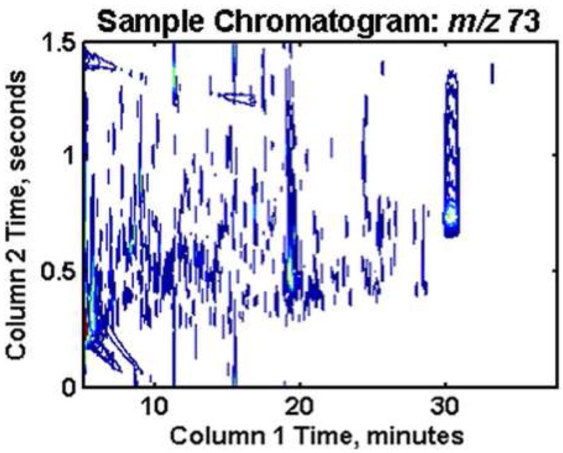
(A) GC × GC–TOF-MS data for typical yeast extract sample at m/z 73. (B) The results at m/z 73 after all 72 GC × GC–TOF-MS chromatograms at this m/z have been analyzed by the Sratio method. (C) As in (B), with Sratios at m/z 128 determined. (D) As in (B), with Sratios at m/z 217. The m/z of 128 and 217 provide more selective information than the global m/z 73. The locations of the metabolites for the more in-depth discussion are enclosed in the boxed regions labeled 1-4, which were identified as methyl citrate, myo-inositol, glucose-6-phosphate and cystathionine, respectively.

At each point in the 2D separation space, a Sratio “mass” spectrum covering all m/z analyzed was obtained to identify the most selective m/z with a good S/N ratio for locating cycling metabolites. The Sratio spectra for the four metabolites in the boxed regions of Figure 3B are shown in Figure 4 A-D. Methyl citrate gave the largest Sratio at 31.5, as indicated in Figure 4A and Table 1. At m/z 73 (the m/z of the most intense fragment) methyl citrate had an average signal to noise (S/N) of 1838 in the two samples with the highest concentration of this particular metabolite. The mass spectrum for methyl citrate was sparse with significant ion fragments at only m/z 73, 147 and 287. In spite of these factors, methyl citrate resulted in three Sratios that have a RSD less than 0.4. The average Sratio calculated using Eq. 2 from the three largest Sratios in Figure 4A (40, 32 and 23) was 32 and the standard deviation of these Sratios was 8. The RSD was calculated by dividing the standard deviation by the average, giving an RSD of 0.3. The RSD threshold was set to remove reagent peaks that had significant signal intensity in one or two m/z but a signal intensity near the limit of detection in most other m/z. The lower Sratios for methyl citrate are due to the Smin noise threshold. Myo-inositol was the second metabolite chosen for more detailed study, with the Sratio spectrum in Figure 4B. The three largest Sratios had an average of 7.4. At first glance it might seem unusual that there is such a large number of m/z with Sratios, when mass spectra seem to have far fewer fragments, however, this can be explained since the Sratio algorithm is not biased by signal intensity, as long as the peak is above the specified noise threshold. Indeed, every m/z in the Sratio spectrum is in the library mass spectrum for myo-inositol. Myo-inositol, in contrast to methyl citrate, has a much stronger S/N and no overlapping interferents, which is evidenced by the many m/z that have similar Sratio values. The glucose-6-phosphate Sratio spectrum in Figure 4C shows an equally complex pattern to that of myo-inositol, with a majority of the mass fragments giving similar Sratio values, with an average of 4.9 for the three largest Sratios. Cystathionine, like methyl citrate, has many fewer m/z with Sratios, as indicated in Figure 4D. At m/z 73 (the m/z of the most intense fragment) the average S/N for cystathionine in the samples with the two largest signals is only 232. However, there remained sufficiently selective m/z with similar Sratios, whereby the three largest were averaged, providing a value of 4.8. This process was continued until all metabolites with a Sratio > 3 per Eq. 2 were located and initially identified using the ChromaTOF software, as summarized in Table 1.

Figure 4.

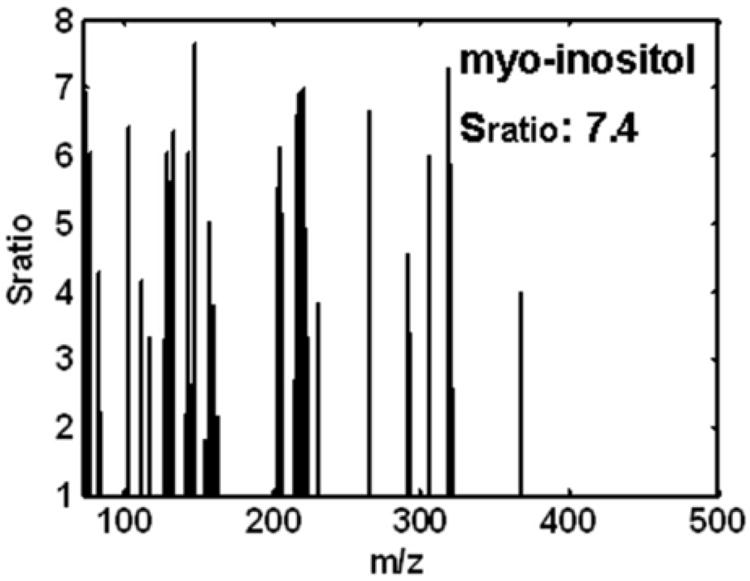
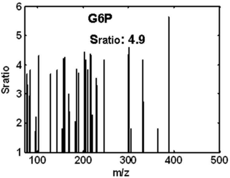
The Sratio “mass” spectra for the four cycling metabolites, numbered 1-4 in Figure 3, in order of decreasing Sratios: (A) methyl citrate, (B) myo-inositol, (C) glucose-6-phosphate (G6P) and (D) cystathionine.

Table 1.

Forty-four metabolites located with a Sratio greater than three.

Metabolite	tR1, min	tR2, s	MV	S/N	Sratio	Vratio
Methylcitrate	19.8	0.64	912	1761	31.5	36.2
Fructose+	20.3	0.36	916	2814	29.8	33.2
Sucrose+	28.5	0.52	890	3378	26.7	17.2
6-Phospho-d-gluconate+	27.9	0.7	838	3325	17.4	13.1
Glycerol-3-phosphate+	18.8	0.97	892	448	9.6	10.1
Glucopyranose	21.6	0.37	803	380	6.2	9.8
Glycerol+	11.3	0.38	947	>10000	12.7	7.4
2-Hydroxy-isovaleric acid	9.4	0.59	932	3074	10.1	6.7
Cystathionine	24.4	0.69	854	207	4.8	4.9
Myo-inositol+	23.0	0.51	923	4914	7.4	4.8
Lysine+	21.0	0.54	931	409	6.6	4.2
Serine+	12.8	0.58	889	6404	5.2	4.1
Norvaline	10.7	0.59	854	116	3.4	4.1
Aspartic acid+	15.4	0.75	957	>10000	5.2	4.0
Lactic acid+	7.5	0.6	945	6775	5.1	3.5
Ornithine	19.6	0.57	936	644	3.8	3.3
Arginine+	16.8	0.56	946	893	4.4	3.2
Succinic acid+	12.0	0.89	941	928	7.0	3.2
Homoserine	14.2	0.56	887	398	3.9	3.0
2-Methylmalic acid	14.6	0.69	862	301	3.8	3.0
Threonic acid	15.7	0.49	899	333	3.4	2.9
2-Aminoadipinic acid	18.2	0.75	837	183	3.3	2.9
Glycine+	11.9	0.59	913	268	4.6	2.8
Glucose+	20.9	0.44	880	413	3.9	2.8
Glycerate-3-phosphate+	19.4	1.16	899	2451	5.8	2.7
Glucose-6-phosphate+	25.5	0.67	945	4584	4.9	2.6
Pyruvate+	7.3	0.56	918	822	4.4	2.6
Trehalose+	30.0	0.75	909	>10000	7.3	2.5
Fumaric acid+	12.7	0.98	935	308	4.3	2.4
3-Hydroxybutanoic acid	9.3	0.62	914	551	3.3	2.3
Ribulose-5-phosphate+	23.3	0.7	826	147	3.3	2.1
Proline+	11.8	0.61	954	3566	4.3	2.1
Luecine+	11.3	0.6	937	2567	3.6	2.0
Alanine+	8.3	0.61	964	>10000	3.1	2.0
Isoleucine+	11.7	0.59	944	4538	3.7	2.0
NAD fragment+	22.2	1.04	878	225	3.2	1.9
Thiamin diphosphate+	17.4	1.29	919	2630	3.9	1.9
d-Ribose-5-phosphate+	23.1	0.71	901	385	3.8	1.9
Valine+	10.3	0.61	954	9703	3.7	1.8
Threonine+	13.2	0.56	957	7977	3.4	1.7
Phenylalanine+	17.0	0.67	933	676	3.2	1.7
UDP glucose & G1P+	18.9	0.43	951	3166	3.8	1.6
Mannitol+	21.1	0.41	926	2417	3.4	1.6
Pseudo uridine	25.7	0.51	783	443	3.3	1.5

The Sratio determined the initial chromatographic locations for study, but the Vratio, obtained after PARAFAC deconvolution, gives a more accurate cycle amplitude. The MV (reverse mass spectral match value) is the average of the two most intense samples after PARAFAC deconvolution. The S/N listed is the average of injection 1 for samples with the two highest signals.

⁺retention time confirmed by standards.

After identifying the location of cycling metabolites using the Sratio method and initial metabolite identification using ChromaTOF software, the PARAFAC GUI was used to confirm identification and accurately quantify metabolites in a true 3D fashion. The resulting volume profiles over all time intervals for the four metabolites studied in depth (using Figures 3 and 4) after PARAFAC quantification are given in Figure 5A-D. These four metabolites all show different patterns over the five hour dO₂ cycle (Figure 1), with the cycling patterns reproduced in the second cycle. The sharp spiking discovered for methyl citrate, Figure 5A, was also observed in a preliminary experiment where metabolite extracts from only one cycle were analyzed. Myo-inositol and cystathionine were more sinusoidal in character than methyl citrate, in Figure 5B and D respectively. They also cycled at the same frequency. However, they were approximately 180° out of phase with each other. Glucose-6-phosphate is interesting in that there appears to be two cycles within one dO₂ cycle, Figure 5C. Glucose-6-phosphate and methyl citrate might not have been located if the Sratio method put frequency constraints on the data. Each of these metabolite profiles were confirmed and were essentially identical to data collected from the preliminary one cycle experiment.

Figure 5.

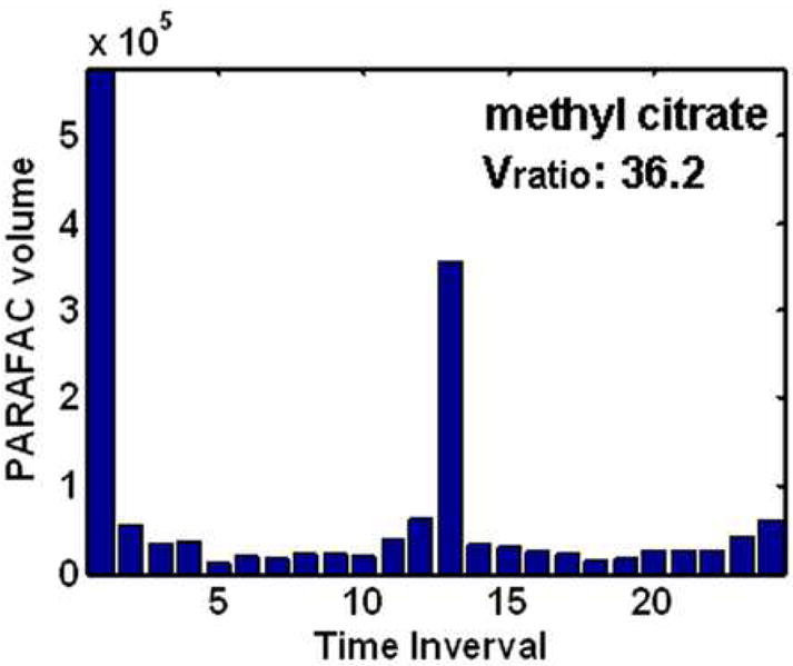
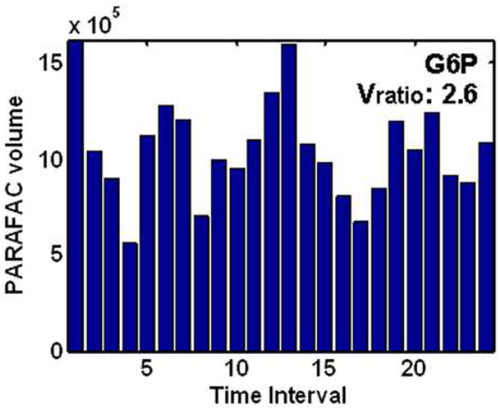
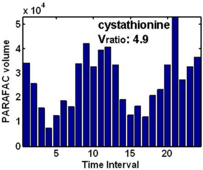
PARAFAC volumes that provide the relative quantification of the four cycling patterns observed in the data for the four metabolites in Figure 4. (A) Methyl citrate exhibited a sharp spiking pattern. (B) Myo-inositol had unimodal oscillations maximizing around time interval 6. (C) Glucose-6-phosphate (G6P) was observed to have bimodal oscillations. (D) Cystathionine exhibited unimodal oscillation directly out of phase with (B) and the dO₂ trace in Figure 1. The PARAFAC GUI also provided the purified mass spectrum for the metabolites for identification.

All identifiable as well as unknown (i.e., unidentified in mass spectral libraries) metabolites with a Sratio greater than three were studied. At this Sratio threshold, 44 identified unique metabolites and 41 unknown metabolites were located, as summarized in Tables 1 and 2. Unknown metabolites are defined as peaks not present in the reagent blanks and with mass spectral features similar to metabolite spectra. The metabolites in the tables are listed in order of descending PARAFAC volume ratio (Vratio). The Vratio calculation is analogous to the Sratio calculated in Eqs. 1 and 2, where the average of the PARAFAC volumes at the two time intervals with largest volumes is divided by the average of the PARAFAC volumes at the two time intervals with the smallest volumes. The Vratios per Eq. 2 for the four metabolites studied in Figures 3 and 4 are indicated in Figure 5. The Vratio is an accurate measure of the depth of modulation. Although the cycling metabolites did give the highest Sratios, a Vratio can be calculated after quantification of each peak using PARAFAC to obtain more accurate cycling amplitude, hence the discrepancy between the Sratios and Vratios for a given metabolite, as indicated in Figures 4 and 5. For a majority of the identified metabolites the Vratio is less than the Sratio, with an average Sratio/Vratio of 1.6. This phenomenon arises from two sources. The first is a slight peak misalignment between samples due to out of phase modulation. Since the Sratio method only retains the peak maxima found after the summation of all samples at each 2D separation time, any specified point that is less than the peak maxima will result in artificially slightly high Sratio results. The second cause for inflated Sratios is interferents. Depending on the resolution of overlapping peaks the raw signal could be more affected at some m/z. Since the Sratio values overestimate the Vratio values ultimately determined, it is instructive to consider the ultimate limit of the Sratio method for distinguishing a cycling metabolite versus one that is not cycling. The critical issue is actually determining the threshold value of the Vratio sufficient to distinguish the patterns (as in Figure 5) different than biological variation. The Vratio threshold was observed to be ~ 1.5 for this study (i.e., the last entry in Table 1). Glucose-6-phosphate in Figure 5C is approaching this Vratio threshold, but is safely above it. At a Vratio ~ 1.5, the metabolite has a cycling “pattern” that is on the edge of randomness.

Table 2.

Locations of forty one unknown metabolites in the both the 2D separation space as well as PCA scores space, listed in order of decreasing Vratio.

Metabolite	tR1, min	tR2, s	Vratio	PC1 score	PC2 score	Group
unk 897	15.0	1.02	18.0	2.15	-1.66	G1
unk 562	9.4	0.39	10.8	1.71	0.30	G4
unk 1288	21.5	0.5	8.6	2.06	0.71	G2
unk 561	9.4	0.41	6.3	2.42	0.18	G4
unk 915	15.3	0.35	6.0	3.74	-0.01	G4
unk 1002	16.7	0.86	6.0	2.81	0.99	G2
unk 832	13.9	0.99	5.7	2.82	1.25	G2
unk 972	16.2	0.59	3.8	3.05	-0.80	G1
unk 1053	17.6	0.4	3.7	2.93	-0.19	G4
unk 711	11.9	0.5	3.6	2.65	-0.09	G4
unk 1207	20.1	0.71	3.6	2.82	-0.63	G1
unk 984	16.4	0.43	3.4	2.11	-0.07	G4
unk 844	14.1	0.44	3.2	2.49	-0.08	G4
unk 970	16.2	0.75	3.2	3.16	-0.88	G1
unk 1227	20.5	0.99	3.2	2.31	0.12	G4
unk 783	13.1	0.54	3.1	3.28	0.90	G2
unk 685	11.4	0.37	3.0	3.47	0.14	G4
unk 634	10.6	0.59	2.9	3.04	0.92	G2
unk 1084	18.1	1.31	2.9	3.72	-0.25	G4
unk 1257	21.0	0.72	2.8	2.96	-0.75	G1
unk 432	7.2	1.22	2.7	3.26	0.18	G4
unk 681	11.4	1.34	2.6	3.49	0.03	G4
unk 567	9.5	0.73	2.5	2.53	-0.02	G4
unk 934	15.6	0.98	2.4	3.67	0.56	G2
unk 1598	26.6	0.67	2.4	3.12	-0.16	G4
unk 1189	19.8	0.51	2.4	3.23	-0.13	G4
unk 1287	21.5	0.68	2.4	3.26	0.37	G4
unk 951	15.9	0.76	2.3	3.41	0.27	G4
unk 982	16.4	0.66	2.1	3.54	0.74	G2
unk 846	14.1	0.53	1.9	3.74	0.51	G2
unk 1046	17.4	1.42	1.8	3.78	-0.12	G4
unk 882	14.7	0.79	1.8	3.46	-0.14	G4
unk 798	13.3	0.59	1.8	3.84	0.06	G4
unk 1990	33.2	1.37	1.7	3.76	-0.11	G4
unk 978	16.3	0.36	1.7	3.64	-0.25	G4
unk 1042	17.4	0.84	1.6	3.79	0.02	G4
unk 910	15.2	1.08	1.6	4.00	0.35	G4
unk 1203	20.1	0.45	1.6	4.11	0.09	G4
unk 1134	18.9	0.57	1.5	4.09	-0.06	G4
unk 1155	19.3	0.54	1.5	4.09	0.02	G4
unk 792	13.2	0.4	1.3	4.27	0.05	G4

The group number corresponds to the clustering described in Figure 6. Unknown metabolites were labeled based on the column 1 retention in seconds.

In addition to the Sratios and Vratios, mass spectral match values (MVs) were also calculated to give an indication of the quality of the identification and are reported in Table 1. The MVs were obtained after a complete mass range PARAFAC deconvolution of the two most intense samples per a given metabolite. These two values were averaged to give the final MV listed in the table. A perfect match is 1000. More than 50% of the metabolites have a MV above 900 and a majority also have confirmed retention times. The retention time confirmation was obtained from an in-house library of standards run under the same instrumental conditions as the samples. To obtain the S/N listed in Table 1, the values ChromaTOF software calculated from the two most concentrated time intervals for each metabolite were averaged. The Sratio method developed to find cycling metabolites is not biased towards peaks of greater S/N and three metabolites in the top ten Vratios have a S/N less than 500. Ribulose-5-phosphate had one of the lowest S/N values at 160 and trehalose one of the largest with an S/N value greater than 10 000.

Following location and quantification of differentiating metabolites, PCA was applied to the PARAFAC volume data (eg., as in Figure 5), to objectively determine which of the metabolites cycled in a similar manner, as shown in Figure 6. Prior to data analysis by PCA, each metabolite peak volume at a given time interval was divided by the largest volume for each metabolite to give a maximum signal of 1. This forced all metabolites to the same intensity range (0-1), i.e., normalizing the data as in Figure 5 to a level playing field, while preserving the depth of modulation for each metabolite. At first glance, the points on the scores plot in Figure 6 appear to be a continuum, but closer inspection reveals that information about the metabolites can be gleaned from both PC1 and PC2. The PC values as well as the grouping for both unknown and known metabolites are reported in Tables 2 and 3, respectively. The first PC captures intensity variations from both the depth-of-modulation and cycling frequency over the 24 time intervals, as indicated in Figure 7A, with only the identified (known) metabolites shown for clarity. The phase information is captured on PC2, as shown in Figure 7B. If one assumes time interval 5 (center of maximum dO₂ signal) is zero and then calculates a phase relative to that time interval, it is readily apparent that metabolites labeled as G2 are more in phase with the dissolved oxygen than the G1 metabolites, which are approximately 180° out of phase. The phase shift described on PC2 can also be seen in Figures 5B, D. Cystathionine, Figure 5D, and myo-inositol, Figure 5B, have approximately the same PC1 score, but are on opposite ends of PC2.

Figure 6.

Classification of the metabolite cycling patterns using PCA. Metabolites were determined to fall into roughly four groups labeled G1, G2, G3 and G4. G1 and G2 are unimodal but primarily out of phase, G3 metabolites show spiking traits and metabolites in G4 are either multimodal or not cycling with a well-defined pattern (i.e., low depth-of-modulation with Vratios approaching 1.5).

Table 3.

Locations of identified metabolites in the PCA scores space, listed in order of decreasing Vratio.

Metabolite	PC1 score	PC2 score	Group	Vratio	ϕ
Methylcitrate	0.69	-0.28	G3	36.2	----
Fructose	0.65	-0.59	G3	33.2	----
Sucrose	1.31	0.46	G3	17.2	----
6-Phospho-d-gluconate	1.66	-0.22	G3	13.1	----
Glycerol-3-phosphate	1.13	-0.39	G3	10.1	----
Glucopyranose	1.51	-0.04	G3	9.8	----
Glycerol	1.43	-0.63	G3	7.4	----
2-Hydroxyisovaleric acid	2.44	1.47	G2	6.7	0
Cystathionine	2.78	-1.01	G1	4.9	150
Myo-inositol	2.59	0.63	G2	4.8	60
Lysine	2.80	-1.07	G1	4.2	120
Serine	2.50	-0.82	G1	4.1	120
Norvaline	2.96	1.21	G2	4.1	30
Aspartic acid	2.99	1.13	G2	4.0	300 (-60)
Lactic acid	2.41	-0.23	G4	3.5	----
Ornithine	3.15	-0.88	G1	3.3	210
Arginine	2.74	-0.62	G1	3.2	210
Succinate	3.16	-0.62	G1	3.2	150
Homoserine	3.25	-0.76	G1	3.0	150
2-Methylmalic acid	2.87	-0.55	G1	3.0	240
Threonic acid	3.27	0.90	G2	2.9	30
2-Aminoadipinic acid	3.10	-0.79	G1	2.9	150
Glycine	2.95	-0.30	G4	2.8	----
Glucose	2.62	-0.10	G4	2.8	----
Glycerate-3-phosphate	3.16	0.24	G4	2.7	----
Glucose-6-phosphate	3.21	-0.12	G4	2.6	----
Pyruvate	3.29	-0.74	G1	2.6	120
Trehalose	3.09	0.44	G2	2.5	60
Fumaric acid	2.94	0.14	G4	2.4	----
3-Hydroxybutanoic acid	3.45	0.70	G2	2.3	0
Ribulose-5-phosphate	3.11	-0.31	G4	2.1	----
Proline	3.42	-0.28	G4	2.1	----
Leucine	3.55	-0.38	G1	2.0	120
Alanine	3.71	-0.04	G4	2.0	----
Isoleucine	3.80	0.56	G2	2.0	60
NAD fragment	3.56	-0.13	G4	1.9	----
Thiamin diphosphate	3.55	-0.04	G4	1.9	----
Ribose-5-phosphate	3.47	-0.19	G4	1.9	----
Valine	3.91	0.06	G4	1.8	----
Threonine	3.56	-0.02	G4	1.7	----
Phenylalanine	3.99	0.27	G4	1.7	----
UDP glucose & G1P	4.07	-0.01	G4	1.6	----
Mannitol	4.12	-0.02	G4	1.6	----
Pseudo uridine	4.02	-0.04	G4	1.5	----

The group number corresponds to the clustering described in Figure 6. The phase, ϕ, was calculated relative to the dissolved oxygen cycle for the metabolites that showed similar periodicity.

Figure 7.

Plots showing the correlation between the PCA scores values from Figure 6 and metabolites. (A) PC1 describes the Vratios. (B) PC2 separates the metabolites based on phase information. The phase was calculated relative to time interval 5 of the dO₂ cycle in Fig. 1.

5. Conclusions

A data processing method termed the Sratio method was developed for 3D GC × GC–TOF-MS data and proven to distinguish chromatographic locations showing changes between a large number of sample classes, in this investigation of cycling metabolites from 24 time interval measurements. The major strength of this reported methodology is that only the most selective m/z were retained for each 2D chromatographic location in order to find sample (i.e., time interval) differentiating locations. Two additional strengths of the Sratio approach are the user’s ability to tune the algorithm to reduce solvent and reagent artifacts as well as obtain one Sratio per chromatographic peak. Issues addressed for proper implementation of this algorithm include the dependence on accurate retention time alignment between samples and the need for a sufficient sampling of the first dimension slices to reconstruct a column 1 peak profile. Following the Sratio method by an accurate quantification tool, in this case PARAFAC, improves determination into the differentiating ability of the located chromatographic sub region. An objective cluster analysis (PCA) then can be used to determine the similarity of samples (studying the cycling patterns). These combined chemometric tools allow the user to gain an accurate understanding of the system under investigation. This method also has potential for the analysis of data exhibiting similar behavior in more than one sample type but large differences between other sample types.

References

- 1.Liu Z, Phillips JB. J Chromatogr Sci. 1991;29:227. [Google Scholar]
- 2.Kinghorn RM, Marriott PJ. J High Resolut Chromatogr. 1998;21:620. [Google Scholar]
- 3.Beens J, Adahchour M, Vreuls RJJ, van Altena K, Brinkman UATh. J Chromatogr A. 2001;919:127. doi: 10.1016/s0021-9673(01)00785-3. [DOI] [PubMed] [Google Scholar]
- 4.Bruckner CA, Prazen BJ, Synovec RE. Anal Chem. 1998;70:2796. [Google Scholar]
- 5.Seeley JV, Kramp F, Hicks CJ. Anal Chem. 2000;72:4346. doi: 10.1021/ac000249z. [DOI] [PubMed] [Google Scholar]
- 6.Giddings JC. Unified Separation Science. Wiley-Interscience; New York: 1991. [Google Scholar]
- 7.Focant J-F, Sjodin A, Patterson DG., Jr J Chromatogr A. 2003;1019:143. doi: 10.1016/j.chroma.2003.07.007. [DOI] [PubMed] [Google Scholar]
- 8.Johnson KJ, Prazen BJ, Olund RK, Synovec RE. J Sep Sci. 2002;25:297. [Google Scholar]
- 9.Beens J, Brinkman UATh. Analyst. 2005;130:123. doi: 10.1039/b407372j. [DOI] [PubMed] [Google Scholar]
- 10.Dimandja J-MD, Grainger J, Patterson DG, Jr, Turner WE, Needham LL. J Exposure Anal Environ Epidemiol. 2000;10:761. doi: 10.1038/sj.jea.7500124. [DOI] [PubMed] [Google Scholar]
- 11.Deursen Mv, Beens J, Reijenga J, Lipman P, Cramers C, Blomberg J. J High Resolut Chromatogr. 2000;23:507. [Google Scholar]
- 12.Mohler RE, Dombek KM, Hoggard JC, Young ET, Synovec RE. Anal Chem. 2006;78:2700. doi: 10.1021/ac052106o. [DOI] [PMC free article] [PubMed] [Google Scholar]
- 13.Sinha AE, Hope JL, Prazen BJ, Fraga CG, Nilsson EJ, Synovec RE. J Chromatogr A. 2004;1056:145. [PubMed] [Google Scholar]
- 14.Pierce KM, Hoggard JC, Hope JL, Rainey PM, Hoofnagel AN, Jack RM, Wright BW, Synovec RE. Anal Chem. 2006;78:5068. doi: 10.1021/ac0602625. [DOI] [PubMed] [Google Scholar]
- 15.Welthagen W, Shellie RA, Spranger J, Ristow M, Zimmermann R, Fiehn O. Metabolomics. 2005;1:65. doi: 10.1016/j.chroma.2005.05.088. [DOI] [PubMed] [Google Scholar]
- 16.Shellie RA, Welthagen W, Zrostlikova J, Spranger J, Ristow M, Fiehn O, Zimmermann R. J Chromatogr A. 2005;1086:83. doi: 10.1016/j.chroma.2005.05.088. [DOI] [PubMed] [Google Scholar]
- 17.Hope JL, Prazen BJ, Nilsson EJ, Lidstrom ME, Synovec RE. Talanta. 2005;65:380. doi: 10.1016/j.talanta.2004.06.025. [DOI] [PubMed] [Google Scholar]
- 18.Sinha AE, Hope JL, Prazen BJ, Nilsson EJ, Jack RM, Synovec RE. J Chromatogr A. 2004;1058:209. [PubMed] [Google Scholar]
- 19.Pichersky E, Gang DR. Trends Plant Sci. 2000;5:439. doi: 10.1016/s1360-1385(00)01741-6. [DOI] [PubMed] [Google Scholar]
- 20.Bino RJ, Hall RD, Fiehn O, Kopka J, Saito K, Draper J, Nikolau BJ, Mendes P, Roessner-Tunali U, Beale MH, Trethewey RN, Lange BM, Wurtele ES, Sumner LW. Trends Plant Sci. 2004;9:418. doi: 10.1016/j.tplants.2004.07.004. [DOI] [PubMed] [Google Scholar]
- 21.Forster J, Famili I, Fu P, Palsson BO, Nielsen J. Genome Res. 2003;13:244. doi: 10.1101/gr.234503. [DOI] [PMC free article] [PubMed] [Google Scholar]
- 22.Dunn WB, Bailey NJC, Johnson HE. Analyst. 2005;130:606. doi: 10.1039/b418288j. [DOI] [PubMed] [Google Scholar]
- 23.Jonsson P, Johansson AI, Gullberg J, Trygg J, A J, Grung B, Marklund S, Sjostrom M, Antti H, Moritz T. Anal Chem. 2005;77:5635. doi: 10.1021/ac050601e. [DOI] [PubMed] [Google Scholar]
- 24.Hollywood K, Brison DR, Goodacre R. Proteomics. 2006;6:4716. doi: 10.1002/pmic.200600106. [DOI] [PubMed] [Google Scholar]
- 25.Goodacre R, Vaidyanathan S, Dunn WB, Harrigan GG, Kell DB. Trends Biotechnol. 2004;22:245. doi: 10.1016/j.tibtech.2004.03.007. [DOI] [PubMed] [Google Scholar]
- 26.Oliver SG, Winson MK, Kell DB, Baganz F. Trends Biotechnol. 1998;16:373. doi: 10.1016/s0167-7799(98)01214-1. [DOI] [PubMed] [Google Scholar]
- 27.Berg RAvd, Hoefsloot HC, Westerhuis JA, Smilde AK, Werf MJvd. BMC Genomics. 2006;7:142. doi: 10.1186/1471-2164-7-142. [DOI] [PMC free article] [PubMed] [Google Scholar]
- 28.Kell DB, Oliver SG. BioEssays. 2004;26:99. doi: 10.1002/bies.10385. [DOI] [PubMed] [Google Scholar]
- 29.Tikunov Y, Lommen A, Vos CHRd, Verhoeven HA, Bino RJ, Hall RD, Bovy AG. Plant Physiol. 2005;139:1125. doi: 10.1104/pp.105.068130. [DOI] [PMC free article] [PubMed] [Google Scholar]
- 30.Sihna AE, Prazen BJ, Synovec RE. Anal Bioanal Chem. 2004;378:1948. doi: 10.1007/s00216-004-2503-7. [DOI] [PubMed] [Google Scholar]
- 31.Johnson KJ, Synovec RE. Chemom Intell Lab Syst. 2001;60:225. [Google Scholar]
- 32.Hoggard JC, Synovec RE. Anal Chem. 2007;79:1611. doi: 10.1021/ac061710b. [DOI] [PubMed] [Google Scholar]
- 33.Wise BM, Gallangher NB, Bro R, Shaver JM, Windig W, Koch RS. PLS_Toolbox 3.5 for use with MATLAB. 2004:123. [Google Scholar]
- 34.Tu BP, Kudlicki A, Rowicka M, McKnight SL. Science. 2005;310:1152. doi: 10.1126/science.1120499. [DOI] [PubMed] [Google Scholar]
- 35.Klevecz RR, Bolen J, Forrest G, Murray DB. Proc Nat Acad Sci U S A. 2004;101:1200. doi: 10.1073/pnas.0306490101. [DOI] [PMC free article] [PubMed] [Google Scholar]
- 36.Murray DB, Beckmann M, Kitano H. Proc Nat Acad Sci U S A. 2007;104:2241. doi: 10.1073/pnas.0606677104. [DOI] [PMC free article] [PubMed] [Google Scholar]
- 37.Castrillo JI, Hayes A, Mohammed S, Gaskell SJ, Oliver SG. Phytochemistry. 2003;62:929. doi: 10.1016/s0031-9422(02)00713-6. [DOI] [PubMed] [Google Scholar]
- 38.Johnson KJ, Wright BW, Jarman KH, Synovec RE. J Chromatogr A. 2003;996:141. doi: 10.1016/s0021-9673(03)00616-2. [DOI] [PubMed] [Google Scholar]
- 39.Andersson CA, Bro R. Chemom Intell Lab Syst. 2000;52:1. [Google Scholar]