Investigation of discrete imaging models and iterative image reconstruction in differential X-ray phase-contrast tomography

Abstract

Differential X-ray phase-contrast tomography (DPCT) refers to a class of promising methods for reconstructing the X-ray refractive index distribution of materials that present weak X-ray absorption contrast. The tomographic projection data in DPCT, from which an estimate of the refractive index distribution is reconstructed, correspond to one-dimensional (1D) derivatives of the two-dimensional (2D) Radon transform of the refractive index distribution. There is an important need for the development of iterative image reconstruction methods for DPCT that can yield useful images from few-view projection data, thereby mitigating the long data-acquisition times and large radiation doses associated with use of analytic reconstruction methods. In this work, we analyze the numerical and statistical properties of two classes of discrete imaging models that form the basis for iterative image reconstruction in DPCT. We also investigate the use of one of the models with a modern image reconstruction algorithm for performing few-view image reconstruction of a tissue specimen.

1. Introduction

Differential phase-contrast tomography (DPCT) employing hard X-rays [1–5] refers to a class of imaging method for reconstructing the X-ray refractive index distribution of objects from knowledge of differential projection data. At hard X-ray energies, variations in the real component of the refractive index distribution of a light- or medium-density material are generally several orders of magnitude larger than are the variations in the imaginary component (i.e., the X-ray absorption). Consequently, DPCT may permit the visualization and quantitation of objects that present very low or no X-ray absorption contrast. In recent years, there have also been advancements [6, 7] in implementing the method on the bench top by use of tube-based X-ray sources. This is particular important in order for DPCT to find widespread use in biomedical and nondestructive imaging applications.

The tomographic projection data in DPCT, from which an estimate of the refractive index distribution is reconstructed, correspond to one-dimensional (1D) derivatives with respect to the detector row coordinate of the two-dimensional (2D) Radon transform of the refractive index distribution. These data can be interpreted as the angles in a plane that is perpendicular to the axis of tomographic scanning by which the probing X-ray beams are deflected by the object due to refraction. Several methods are available for implementing DPCT by use of synchrotron-or tube-based X-ray sources. Such methods include those based on diffractive optics [8, 9] or interferometry [10]. When DPCT is implemented with optical wavefields, which has been referred to as beam-deflection tomography [11], techniques such as moire deflectometry [12] have been employed for measuring the beam-deflection data.

It has been demonstrated that image reconstruction in DPCT can be achieved by use of modified filtered backprojection (FBP) algorithms [11, 13, 14]. An important observation by Faris and Byer [11] was that the 1D differentiation of the projection data is prescribed by the classic FBP algorithm. Accordingly, instead of integrating the differential projection data explicitly and then applying the classic FBP algorithm for reconstruction, they proposed a deflection filtered backprojection DFBP algorithm that acts directly on the differential projection data. In order to avoid image artifacts when employing this algorithm and other analytic reconstruction algorithms, tomographic measurements must be typically be acquired at a large number of view angles. This is highly undesirable because it can result in long data-acquisition times, especially in bench top applications where the X-ray tube power is limited, and also may damage the sample due to the large radiation exposure. Iterative image reconstruction algorithms have been widely employed in mature tomographic imaging modalities for mitigating data-incompleteness and noise. However, there is a scarcity of studies of iterative image reconstruction in DPCT [6, 15] and there remains an important need to develop robust iterative reconstruction methods for this modality.

In this work, we analyze the numerical and statistical properties of two classes of discrete imaging models that form the basis for iterative image reconstruction in DPCT. The models differ in the choice of expansion functions that are employed to discretize the infinite-dimensional refractive index distribution that one seeks to estimate. One model employs conventional pixel expansion functions while the other employs Kaiser-Bessel window functions. The latter choice is shown to have the attractive feature that the 1D derivative operator in the DPCT imaging model can be computed analytically, thereby cirvumventing the need to numerically approximate it. This feature has also recently been identified by Köhler, et al. [15]. A modern iterative reconstruction algorithm that seeks to minimize total variation (TV) -norm of the refractive index estimate is employed with a discrete imaging model for few-view image reconstruction. The effectiveness of the reconstruction method is demonstrated by use of experimental DPCT projection data corresponding to a biological tissue specimen.

2. Background: Imaging model for differential X-ray phase-contrast tomography

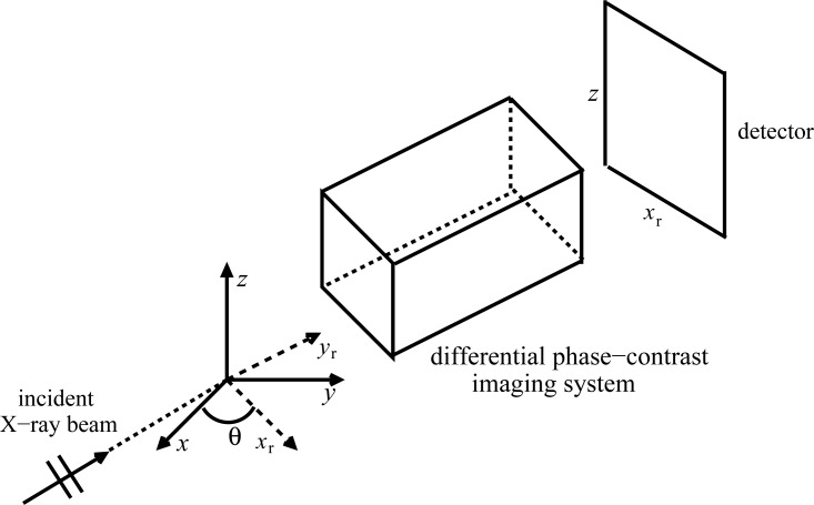
We will utilize the parallel-beam tomographic scanning geometry depicted in Fig. 1. However, the results that follow can readily be adapted to the case of spherical wave illumination in the paraxial limit [7]. The z-axis of the reference coordinate system (x,y,z) defines the axis of rotation of the tomographic scanning. The rotated coordinate system (x_r, y_r, z) is related to the reference system by by x_r = x cosθ + ysinθ, y_r = y cosθ − xsinθ, where θ ∈ [0,π) is the tomographic view angle measured from the positive x-axis. A phase-amplitude object positioned at the origin is irradiated by an X-ray plane-wave with wavelength λ, or equivalently wavenumber $k=\genfrac{}{}{0.1ex}{}{2\pi }{\lambda }$, which propagates in the direction of the positive y_r-axis.

Fig. 1.

A schematic of differential phase-contrast imaging tomography. The black box represents the system of optical elements that is specific to the implementation.

2.1. Data function and imaging model in continuous form

Let δ(x,y,z) ≡ 1 − n(x,y,z) denote the compactly supported and bounded object function we seek to reconstruct, where n(x,y,z) is the real-valued refractive index distribution. We will employ the notation δ(r₂; z) ≡ δ(x,y,z), where r₂ = (x, y), as a convenient description of a transverse slice of the 3D object function.

In DPCT employing a grating interferometer [1, 8, 10, 16, 17] or X-ray crystal optics [9,18–24], the wavefield transmitted through the object is perturbed by one or more optical elements. The intensity of the perturbed wavefield at view angle θ is measured in the (x_r, z) plane located at y_r = d and will be denoted by I(x_r, z,θ;K). Here K represents an integer-valued index that specifies the state of the imaging system. For example, in crystal analyzer-based systems, distinct values of K would correspond to different orientations of the analyzer crystal. Alternatively, in grating interferometry when a phase-stepping procedure [1, 8] is employed, distinct values of K correspond to different translational positions of the grating that is being scanned.

From knowledge of ${\left\{I\left(x_r,z,\theta ;k\right)\right\}}_{K=1}^{N_K}$ with N_K ≥ 1, methods are available [1, 25, 26] for computing a data function g(x_r, z,θ) that, for a fixed value of z, is related to the sought-after object function δ(r₂; z) as

$$g(x_r,\theta ;z)=\genfrac{}{}{0.1ex}{}{\partial }{\partial x_r}{\int }_{\infty }d{y}_r\delta ({\mathbf{r}}_2;z)\equiv \genfrac{}{}{0.1ex}{}{\partial }{\partial x_r}\mathbf{R}\delta ({\mathbf{r}}_2;z).$$ (1)

Here, R denotes the 2D Radon transform operator. Equation (1) represents an idealized imaging model for DPCT in its continuous form that assumes a geometrical optics approximation. A discussion of the validity of this approximation is provided in Chapter 2 of reference [27]. Note that the right hand side of Eq. (1) corresponds to a stack, along the z-axis, of differentiated 2D Radon transforms of δ(r₂; z). The coordinate z can be interpreted as a parameter that specifies a transverse slice and therefore the 3D imaging model can be described by a collection of 2D ones.

The image reconstruction task in DPCT is to determine an estimate of δ(r₂; z) from knowledge of g(x_r,θ;z). When g(x_r,θ;z) is measured at a large number of view angles θ, this can be accomplished by use of analytic image reconstruction algorithms [11,28]. However, in the case of noisy and/or few-view measurement data, analytic reconstruction methods are known to be suboptimal and the use of iterative methods is warranted. The construction and investigation of discrete imaging models that form the basis for iterative image reconstruction in DPCT is described in the remainder of the article.

2.2. General forms of discrete imaging models

A natural way to obtain a discrete imaging model is to discretize the continuous model in Eq. (1). When a digital detector is employed, the measured intensity data and associated data function correspond to an ordered collection of numbers rather than a function of a continuous variable. We will denote the discrete data function as

$$g[s,t;h]\equiv {g(x_r,\theta ;z)|}_{x_r=s{\mathrm{\Delta }}_d,\theta =t{\mathrm{\Delta }}_{\theta },z=h{\mathrm{\Delta }}_d},$$ (2)

where s and h are integer-valued detector element indices and t is the tomographic view index. Here, ${\mathrm{\Delta }}_d=\genfrac{}{}{0.1ex}{}{L}{Q}$ denotes the detector element dimension in a square detector array of dimension L × L, and Q denotes the number of samples measured in each dimension. The quantity Δ_θ denotes the angular sampling interval between the uniformly distributed view angles. The reconstruction algorithms described below can be applied in the case of non-uniformly sampled measurement data as well. The general forms of the reconstruction algorithms would remain unchanged for the case of non-uniformly sampled measurement data; However, the explicit forms of the system matrices would be changed. Although not indicated in Eq. (2), the measured discrete data will also be degraded by the averaging effects of the sampling aperture. Additionally, the effects of finite temporal and spatial beam coherence will effectively blur the data function g[s,t;h]. These effects can limit the attainable spatial resolution in the reconstructed DPCT images. Because the reconstruction problem is inherently 2D, we will consider the problem of reconstructing a transverse slice of the object function located at z = hΔ_d. Let the vector g ∈ 𝕉^M denote a lexicographically ordered representation of g[s,h,t]. The dimension M is defined by the product of the number of detector row elements and the number of view angles.

Many iterative image reconstruction algorithms require a finite-dimensional approximate representation of the object function. A linear N-dimensional approximation of δ(r₂; z = hΔ_d) can be formed as

$${\delta }_a({\mathbf{r}}_2;z=h{\mathrm{\Delta }}_d)=\sum _{n=0}^{N-1}{\mathbf{b}}_n^h{\varphi }_n({\mathbf{r}}_2),$$ (3)

where the subscript a indicates that δ_a(r₂; z) is an approximation of δ(r₂; z), {ϕ_n(r₂)} are a set of expansion functions, and { ${\mathbf{b}}_n^h$} are the corresponding expansion coefficients that depend on the slice index h. Let the 2D function δ_a(r₂; z = hΔ_d) be contained within a disk of radius r₀. The discrete data function satisfies

$$g[s,t;h]\approx {\genfrac{}{}{0.1ex}{}{\partial }{\partial x_r}\mathbf{R}{\delta }_a({\mathbf{r}}_2;z=h{\mathrm{\Delta }}_d)|}_{x_r=s{\mathrm{\Delta }}_d,\theta =t{\mathrm{\Delta }}_{\theta }},$$ (4)

assuming that Rδ_a(r₂; z = hΔ_d) is differentiable ∀x_r ∈ (−r₀, r₀). For certain choices of the expansion functions, such as the pixels described below, this differentiability requirement will not be met. Moreover, when computing Eq. (4), as required by iterative image reconstruction algorithms, the operator $\genfrac{}{}{0.1ex}{}{\partial }{\partial x_r}$ will generally be replaced by a numerical approximation. For use in these cases, a modified version of Eq. (4) is given by

$$g[s,t;h]\approx {\genfrac{}{}{0.1ex}{}{\partial }{\partial x_r}\mathbf{S}\mathbf{R}{\delta }_a({\mathbf{r}}_2;z=h{\mathrm{\Delta }}_d)|}_{x_r=s{\mathrm{\Delta }}_d,\theta =t{\mathrm{\Delta }}_{\theta }},$$ (5)

where S is a smoothing operator that acts with respect to the x_r coordinate and ensures that SRδ_a(r₂; z = hΔ_d) is differentiable. The composite operator $\genfrac{}{}{0.1ex}{}{\partial }{\partial x_r}\mathbf{S}$ can be interpreted as a regularized derivative operator.

In the special case where Rϕ_n(r₂) is differentiable ∀x_r ∈ (−r₀, r₀), as satisfied by the Kaiser-Bessel expansion functions investigated below, Eq. (4) can be expressed as

$$g[s,t;h]\approx \sum _{n=0}^{N-1}{\mathbf{b}}_n^h\genfrac{}{}{0.1ex}{}{\partial }{\partial x_r}\left(\mathbf{R}{\varphi }_n({\mathbf{r}}_2)\right){(x_r,\theta )|}_{x_r=s{\mathrm{\Delta }}_d,\theta =t{\mathrm{\Delta }}_{\theta }}.$$ (6)

In matrix form, each of Eqs. (4)–(6) can be expressed as

$$\mathbf{g}=\mathbf{H}\mathbf{b},$$ (7)

where g is a lexicographically ordered representation of the sampled data function, H is an M × N system matrix, and b is a N × 1 vector of expansion coefficients that has an n-th element given by ${\mathbf{b}}_n^h$.

Equations (5) or (6) describe discrete imaging models for DPCT that can be employed with iterative image reconstruction algorithms for estimation of b from knowledge of g and H. From the estimated b, the object function estimate - the sought after image - can be obtained by use of Eq. (3). In the special case in which the expansion functions are classical pixels, the estimates of b and δ_a(r₂; z = hΔ_d) coincide. Explicit forms for the system matrix H are found by specifying the expansion functions ϕ_n(r₂) and implementation of the operator $\genfrac{}{}{0.1ex}{}{\partial }{\partial x_r}\mathbf{R}$ or $\genfrac{}{}{0.1ex}{}{\partial }{\partial x_r}\mathbf{S}\mathbf{R}$.

Below, we investigate the use of two different choices of expansion functions: the pixel basis function and Kaiser-Bessel window functions. Because the 3D reconstruction problem corresponds to a stack of 2D ones, we will focus on the reconstruction of a transverse slice of constant z = hΔ_d and the discrete index h will be suppressed hereafter. For use with the pixel basis functions, three different discrete implementations of the operator $\genfrac{}{}{0.1ex}{}{\partial }{\partial x_r}\mathbf{S}\mathbf{R}$ are implemented and system matrices are established according to Eq. (5). For the case of the Kaiser-Bessel window expansion functions, the operator $\genfrac{}{}{0.1ex}{}{\partial }{\partial x_r}\mathbf{R}{\varphi }_n({\mathbf{r}}_2)$ can be computed analytically and system matrices are established according to Eq. (6).

3. Construction of system matrices for iterative image reconstruction in DPCT

3.1. System matrix construction employing pixel basis functions

The classic pixel is a commonly employed expansion function and is defined as

$${\varphi }_n^{\mathit{pixel}}({\mathbf{r}}_2)=\text{rect}\left(\genfrac{}{}{0.1ex}{}{x-x_n}{\varepsilon }\right)\text{rect}\left(\genfrac{}{}{0.1ex}{}{y-y_n}{\varepsilon }\right),$$

where rect(x) = 1 for $\left|x\right|\le \genfrac{}{}{0.1ex}{}{1}{2}$ and zero elsewhere, (x_n, y_n) specifies the coordinate of the nth lattice point on a uniform Cartesian lattice, and ɛ is the spacing between those lattice points. A description of the system matrix construction for use with pixel expansion functions provided below. According to Eq. (5), this will require specifying methods for : (1) numerically approximating Rδ_a(r₂; z) and (2) computing a regularized discrete derivative operator $\genfrac{}{}{0.1ex}{}{\partial }{\partial x_r}\mathbf{S}$.

Numerous standard numerical methods are available to compute approximations of Rδ_a(r₂; z) [29–31]. Most of these numerical methods compute the projection data as

$$p[s,t]\equiv \left(\mathbf{R}{\delta }_a({\mathbf{r}}_2)\right)[s,t]=\left(\mathbf{R}{\delta }_a({\mathbf{r}}_2)\right){(x_r,\theta )|}_{x_r=s{\mathrm{\Delta }}_d,\theta =t{\mathrm{\Delta }}_{\theta }}\approx \sum _{j=0}^{N-1}{w}_{stj}{b}_j,$$ (8)

where w_stj is the weighting factor that corresponds to the contribution of the j-th expansion function to the projection data recorded at detector location [s,t], and b_j is the j-th component of b. By defining p ∈ 𝕉^M to be a lexicographically ordered representation of p[s,t], Eq. (8) can be expressed in matrix form as

$$\mathbf{p}={\mathbf{H}}^R\mathbf{b},$$ (9)

where

$${\left[{\mathbf{H}}^R\right]}_{m=t\times S+s,n}=w_{stn},$$ (10)

in which S is the total number of discrete projection data for each view and the notation [H^R]_m,n denotes the element of H^R corresponding to the m-th row and n-th column. In our numerical studies, we adopted a ’ray-driven’ method to establish H^R [30].

We adopted a meshfree method known as smoothed particle hydrodynamics (SPH) [32, 33] for implementing $\genfrac{}{}{0.1ex}{}{\partial }{\partial x_r}\mathbf{S}$. Let p′ ∈ 𝕉^M denote a 1D discrete derivative of p that approximates samples of $\genfrac{}{}{0.1ex}{}{\partial }{\partial x_r}\mathbf{S}\mathbf{R}{\delta }_a({\mathbf{r}}_2;z=h{\mathrm{\Delta }}_d)$. The SPH method determines p′ as

$$p_k^{\text{'}}=\genfrac{}{}{0.1ex}{}{1}{{\rho }_k}\sum _{i=k-K/2}^{i=k+K/2}(p_i-p_k)\genfrac{}{}{0.1ex}{}{\partial \mathbf{W}(d_i-d_k,h)}{\partial x_r},$$ (11)

where p′_k is the k-th element of p′, K is the total number of neighbouring particles, p_i and p_k are the i-th and k-th elements of p respectively, and W(x_r, h) is a kernel function with a smoothing length h. In our studies we employed three different kernel functions of the form: linear, quadratic spline, and cubic spline [32, 33]. Explicit forms of the kernels are provided in the appendix. The density factor ρ_k is defined as

$${\rho }_k=\sum _{i=k-K/2}^{i=k+K/2}\mathbf{W}(d_i-d_k,h).$$ (12)

In matrix form, Eq. (11) is expressed as

$${\mathbf{p}}^{\mathbf{\prime }}={\mathbf{H}}^D\mathbf{p},$$ (13)

where explicit forms of H^D are provided in the appendix that correspond to different choices of W(x_r, h).

By use of Eqs. (9) and (13), the discrete imaging models for the case of pixel expansion functions are obtained as

$$\mathbf{g}\approx {\mathbf{p}}^{\mathbf{\prime }}={\mathbf{H}}^{\mathit{pixel}}\mathbf{b},$$ (14)

where

$${\mathbf{H}}^{\mathit{pixel}}\equiv {\mathbf{H}}^D{\mathbf{H}}^R.$$ (15)

The system matrix H^pixel is generally sparse, since only a few expansion functions contribute to one specific projection value p_i.

3.2. System matrix construction employing generalized Kaiser-Bessel window functions

For Kaiser-Bessel window expansion functions, referred to hereafter as “blobs” [34, 35], $\genfrac{}{}{0.1ex}{}{\partial }{\partial x_r}\mathbf{R}{\varphi }_n({\mathbf{r}}_2)$ is continuous and can be computed analytically. In this case, Eq. (6) can be employed to establish the system matrix in which the derivative and Radon transform operators can be computed accurately.

The blob expansion functions are defined as

$${\varphi }_n^{\mathit{blob}}({\mathbf{r}}_2;m,a,\alpha )=\{\begin{array}{ll}\multicolumn{1}{c}{\genfrac{}{}{0.1ex}{}{{\left[\sqrt{1-{\left(r_b/a\right)}^2}\right]}^m{I}_m\left[\alpha \sqrt{1-{\left(r_b/a\right)}^2}\right]}{I_m(\alpha )},}& \multicolumn{1}{c}{{\mathbf{r}}_b\le a}\\ \multicolumn{1}{c}{0,}& \multicolumn{1}{c}{\text{otherwise},}\end{array}$$ (16)

where I_m(·) is the m-th order modified Bessel function, r_b ≡ |r₂ – r_n| with r_n = (x_n, y_n) denoting the blob center, and a and α determine the blob’s radius and specific shape.

Let ξ ≡ x_r – x_n cosθ – y_n sinθ. As demonstrated by Lewitt [34], the 2D Radon transform of one window function is given by

$$\mathbf{R}{\varphi }_n^{\mathit{blob}}({\mathbf{r}}_2;m,a,\alpha )=\genfrac{}{}{0.1ex}{}{a}{I_m(\alpha )}{\left(\genfrac{}{}{0.1ex}{}{2\pi }{\alpha }\right)}^{1/2}{\left[\sqrt{1-{\left(\xi /a\right)}^2}\right]}^{m+1/2}{I}_{m+1/2}\left(\alpha \sqrt{1-{\left(\xi /a\right)}^2}\right),$$ (17)

for |ξ| ≤ a and zero otherwise. As derived in Appendix B, the 1D derivative of this quantity is given by

$$\genfrac{}{}{0.1ex}{}{\partial \left(\mathbf{R}{\varphi }_n^{\mathit{blob}}({\mathbf{r}}_2;m,a,\alpha )\right)}{\partial x_r}=-\genfrac{}{}{0.1ex}{}{{\left(2\pi \alpha \right)}^{1/2}}{I_m(\alpha )}\genfrac{}{}{0.1ex}{}{\xi }{a}{\left(\sqrt{1-{\left(\xi /a\right)}^2}\right)}^{m-1/2}{I}_{m-1/2}\left(\alpha \sqrt{1-{\left(\xi /a\right)}^2}\right).$$ (18)

By use of Eqs. (18) and (6) the discrete imaging model is given by

$$\begin{array}{l}\multicolumn{1}{c}{g[s,t]\approx -\genfrac{}{}{0.1ex}{}{{\left(2\pi \alpha \right)}^{1/2}}{I_m(\alpha )}}\\ \multicolumn{1}{c}{\times \sum _{n=0}^{N-1}{\mathbf{b}}_n\genfrac{}{}{0.1ex}{}{\xi }{a}{\left(\sqrt{1-{\left(\xi /a\right)}^2}\right)}^{m-1/2}{I_{m-1/2}\left(\alpha \sqrt{1-{\left(\xi /a\right)}^2}\right)|}_{\xi =s{\mathrm{\Delta }}_d-x_n\text{cos}(t{\mathrm{\Delta }}_{\theta })-y_n\text{sin}(t{\mathrm{\Delta }}_{\theta })},}\end{array}$$ (19)

or, in matrix form,

$$\mathbf{g}\approx {\mathbf{H}}^{\mathit{blob}}\mathbf{b},$$ (20)

where

$$\begin{array}{l}\multicolumn{1}{c}{{\left[{\mathbf{H}}^{\mathit{blob}}\right]}_{m^{\prime },n}={\left[{\mathbf{H}}^{\mathit{blob}}\right]}_{m^{\prime }=t\times S+s,n}=-\genfrac{}{}{0.1ex}{}{{\left(2\pi \alpha \right)}^{1/2}}{I_m(\alpha )}}\\ \multicolumn{1}{c}{\times \genfrac{}{}{0.1ex}{}{\xi }{a}{\left(\sqrt{1-{\left(\xi /a\right)}^2}\right)}^{m-1/2}{I_{m-1/2}\left(\alpha \sqrt{1-{\left(\xi /a\right)}^2}\right)|}_{\xi =s{\mathrm{\Delta }}_d-x_n\text{cos}(t{\mathrm{\Delta }}_{\theta })-y_n\text{sin}(t{\mathrm{\Delta }}_{\theta })},}\end{array}$$ (21)

and S is the total number of discrete projection data for each view. Similar to the pixel case, the system matrix H^blob is sparse because only a relatively few blobs contribute to each component of g.

Note that the k-th order spatial derivative of ${\varphi }_n^{\mathit{blob}}({\mathbf{r}}_2;m,a,\alpha )$ is continuous when m > k [34]. In the studies below, m = 2 was chosen. This ensured that the first-order derivatives of the blobs were continuous.

4. Comparison of numerical and statistical properties of system matrices

4.1. SVD analysis of the system matrices

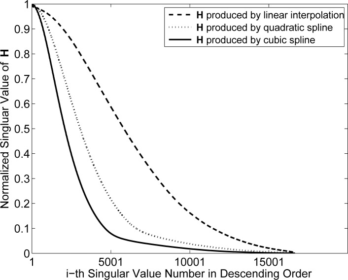
In order to investigate how the different expansion functions influence the numerical properties of the imaging models described in Sections 3.1 and 3.2, the singular value decomposition (SVD) was employed. Specifically, the rates of decay of the singular values associated with the different system matrices were examined to gain insights into the stability of the associated reconstruction problems. It is well-known that the stability of a reconstruction problem is adversely affected by a rapid decay of singular values [36]. For the pixel basis function, three system matrices H^pixel were constructed as described in Sec. 3.1 for the cases where linear, quadratic spline, and cubic spline kernel functions W(x_r, h) were employed [32, 33, 37]. Explicit forms of three kernels are provided in the appendix. The scanning configuration assumed 180 equally spaced tomographic views and 256 samples along the detector array. The detector pixel pitch was 25 μm. The window size of h was chosen to be two times detector pixel pitch, three times detector pixel pitch, and four times detector pixel pitch for linear interpolation, quadratic spline and cubic spline kernel, respectively. The object was assumed to be contained within an area of dimension 6.4 mm × 6.4 mm. For the pixel-based studies, a 128 × 128 array of 50 μm square pixels was employed to discretize the object. Accordingly, the system matrices H^pixel were of dimension 46080 (256 × 180) by 16384 (128 × 128). For the case of blob expansion functions, the same scanning configuration was considered. Six system matrices H^blob were constructed as described in Sec. 3.2 for the cases where the blob parameters were chosen as m = 2, radius a = 75 μm (1.5 times sampling interval) or 100 μm (2 times sampling interval), and α = 2, 6, or 10.4. Hereafter, we will refer to the blob radius relative to the image grid spacing. For example, we use indicate a = 1.5 to represent a physical radius of 75 μm and a = 2 to represent a physical radius of 100μm. The value of α = 10.4 was chosen because it results in a quasi-bandlimited blob function that has been demonstrated to suppress artifacts in other tomographic image reconstruction applications [35,38]. Similar values were employed in references [39, 40]. The distance between the centers of two neighboring blobs was fixed at 50 μm. The dimension of H^blob is the same as that of H^pixel. The spectrum of singular values was computed for all system matrices using the Matlab programming environment [41].

Figures 2 – 4 display the computed normalized singular value spectra. Figure 2 shows the normalized singular spectra for the different system matrices H^pixel for the three different weighting kernels. The matrix constructed by use of the cubic spline kernel is the most ill-conditioned, while the system matrix constructed by use of the linear kernel is the least ill-conditioned. This behavior is expected since the cubic spline kernel imposes the most smoothness on the data, followed by the quadratic spline and linear kernels.

Fig. 2.

Singular value spectra associated with the system matrices H^pixel with pixel size 50 μm.

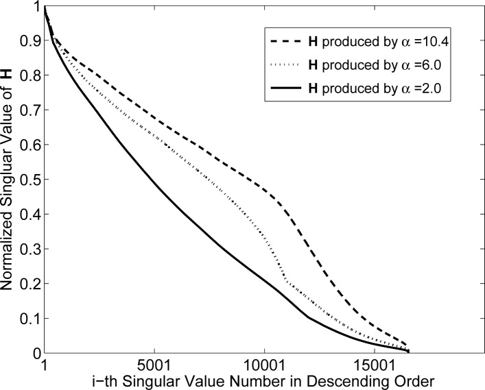
Fig. 4.

Singular value spectra associated with the system matrices H^blob with m = 2, relative radius a = 2 (physical size 100μm).

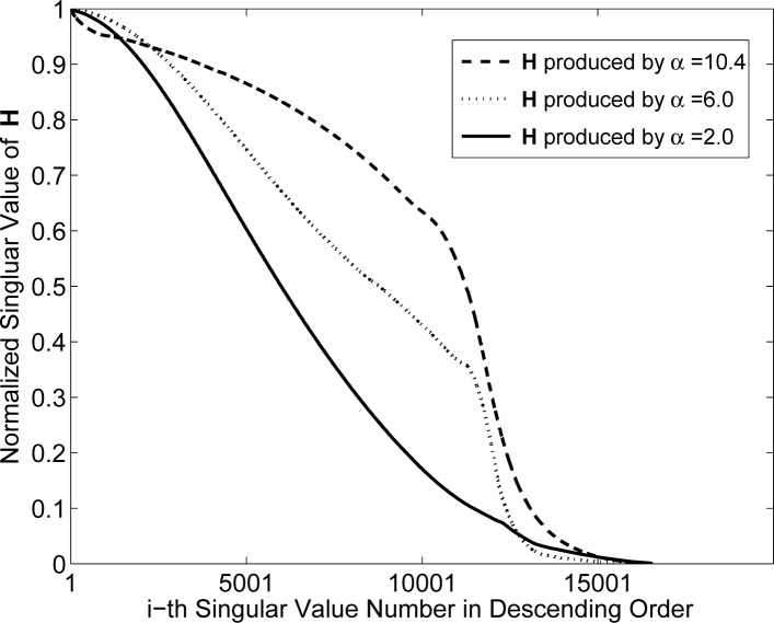
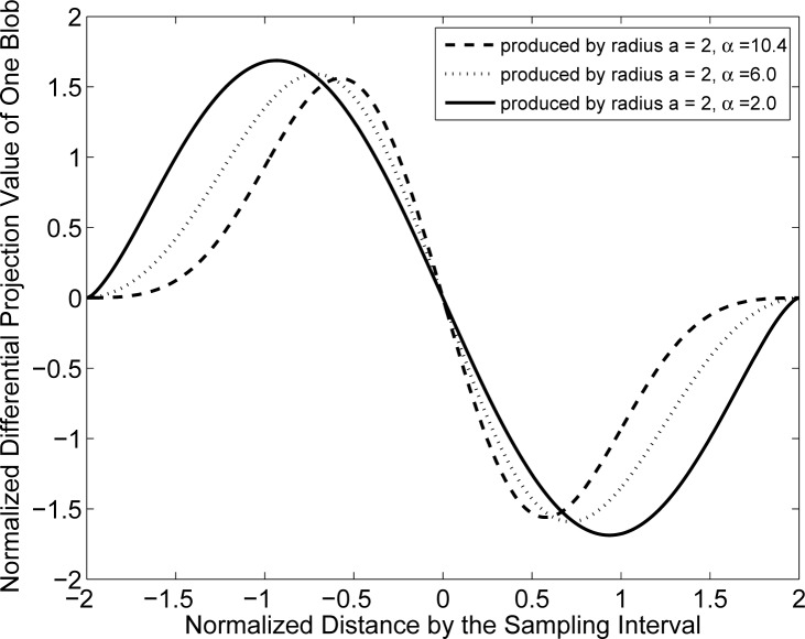
The spectra for the blob system matrices are shown in Figs. 3 and 4. Figure 3 displays the spectra when the blobs had a relative radius a = 1.5 and varying shape parameter α. These results indicate that the parameter α will generally affect the stability of the system matrix. In this case, α = 2.0 corresponds to the most poorly conditioned system matrix while α = 10.4 corresponds to the best conditioned system matrix. The spectra for the case when the blob relative radius a was increased to 2 (physical size 100 μm) are displayed in Fig. 4. The parameter α is again observed to have a significant effect on the stability of the system matrices. The system matrix corresponding to α = 2 is the most ill-conditioned, while the one corresponding to α = 10.4 is the least ill-conditioned. In order to gain insight into this behavior, one can examine the normalized differential projection profile of one blob as shown in Fig. 5. One observes that the profile is more localized when α increases from 2 to 10.4, which results in a better conditioned system matrix.

Fig. 3.

Singular value spectra associated with the system matrices H^blob with m = 2, relative radius a = 1.5 (physical size 75μm).

Fig. 5.

Profiles of the differential projection value of one blob with m = 2, relative radius a = 2.

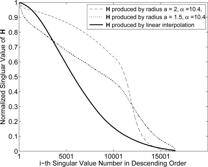
In order to facilitate the comparison of the pixel- and blob-based results, the three highest singular value spectra from Figs. 3–5 were re-plotted together in Fig. 6. Two of these spectra correspond to different H^blob with α = 10.4. and relative radius a = 1.5 and a = 2 and the third to H^pixel employing the linear weighting kernel. The two blob-based spectra possess a slower rate of decay than the pixel-based spectra, indicating that that the blob-based system matrices will yield more stable reconstruction problems than will pixel-based ones.

Fig. 6.

The three highest singular value spectra are replotted for comparison. Two of the spectra correspond to H^blob with α = 10.4, relative radius a = 1.5 and a = 2. The third spectra corresponds to H^pixel based on the linear weighting kernel.

4.2. Investigation of image variance and spatial resolution

Computer-simulation studies were conducted to investigate the trade-offs between image variance and spatial resolution for images reconstructed by use of the different system matrices.

4.2.1. Simulation data and image reconstruction algorithm

The 2D numerical phantom displayed in Fig. 7 was employed to represent our object function δ(r₂; z). The physical size of the phantom was 25.6 mm × 25.6 mm. The phantom was composed of nine uniform disks possessing different values and physical sizes, which were blurred with a Gaussian kernel of width 0.15 mm. From knowledge of the phantom, the elements of the differential projection data g were computed analytically. The scanning geometry employed assumed 180 tomographic views that were uniformly spaced over a π angular range. At each view, the detector was assumed to possess 1024 elements of pitch 25 μm.

Fig. 7.

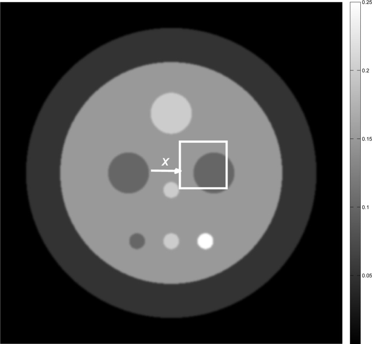
The numerical phantom employed in our simulation studies with an ROI indicated

There are several sources of noise in X-ray DPCT [42] that include phase stepping jitter, quantum noise, and noise from the detection electronics. One hundred noisy data vectors were computed as realizations of an uncorrelated zero-mean Gaussian random vector [43]. The standard deviation σ_n of each element of the random vector was constant and was set according to the rule σ_n = 0.2|g|_mean, where ${\left|\mathbf{g}\right|}_{\mathit{mean}}=\genfrac{}{}{0.1ex}{}{1}{M}{\sum }_{m=1}^M\left|g_m\right|$ with g_m denoting the m-th component of the noiseless data vector g.

From the 100 noisy differential projection data vectors, the penalized least-squares (PLS) algorithm described in reference [44] was employed to reconstruct 100 noisy coefficient estimates b̂. The analytic solution of the PLS algorithm with L₂ regularization can be written as a pseudo-inverse operator H⁺ acting on g. The pseudo-inverse operator H⁺ can be decomposed as a linear combination of certain outer-product operators, whose coefficients are the reciprocals of the singular values of the operator H [36, 45] that were analyzed in Sec. 4.1. The estimates b̂ represent approximate solutions of the optimization program

$$\widehat{\mathbf{b}}=\underset{\mathbf{b}}{\text{arg}\hspace{0.17em}\text{min}}\Vert \mathbf{g}-\mathbf{H}\mathbf{b}\Vert +\gamma L(\mathbf{b}),$$ (22)

where γ is a regularization parameter,

$$L(\mathbf{b})=\sum _{n=0}^{N-1}{\sum _{k\in {𝒩}_n}\left({\left[\mathbf{b}\right]}_n-{\left[\mathbf{b}\right]}_k\right)}^2,$$ (23)

with the set 𝒩_n containing the index values of the four neighbour points of the nth value of b. From knowledge of b̂, estimates of the object function δ_a(r₂; z) were obtained by use of Eq. (3). For the cases where blob expansion functions were employed, the estimates of δ_a(r₂; z) were sampled by use of a 2D Dirac delta sampling function onto a Cartesian grid and the resulting values stored as a matrix for analysis and display.

Sets of images were reconstructed by use of different system matrices H^pixel or H^blob. For the pixel-based studies, the object was represented by a 512 × 512 pixel array with a 50 μm pitch. Three different pixel-based matrices H^pixel were constructed corresponding to the weighting kernel functions described in Sec. 3.1. For the blob-based studies, six different system matrices were employed that corresponded to blob parameters relative radius a = 1.5 (physical size 75 μm), relative radius a = 2 (physical size 100 μm), and α = 2, 6, or 10.4. In all cases, 512 × 512 blobs were employed to represent the object function and the distance (sampling interval) between the blobs was 50 μm. For each system matrix, five sets of 100 noisy images were reconstructed for distinct values of the regularization parameter specified by γ = 10, 200, 1000, 2000, or 5000.

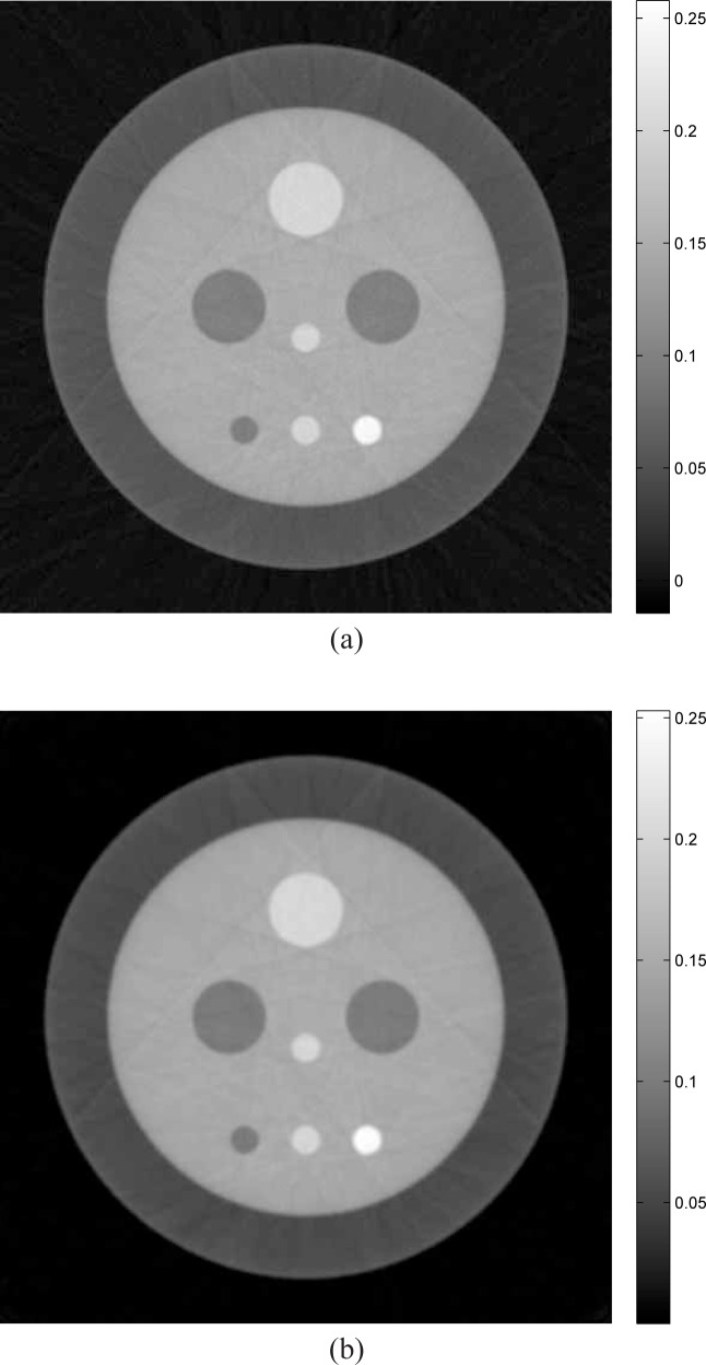
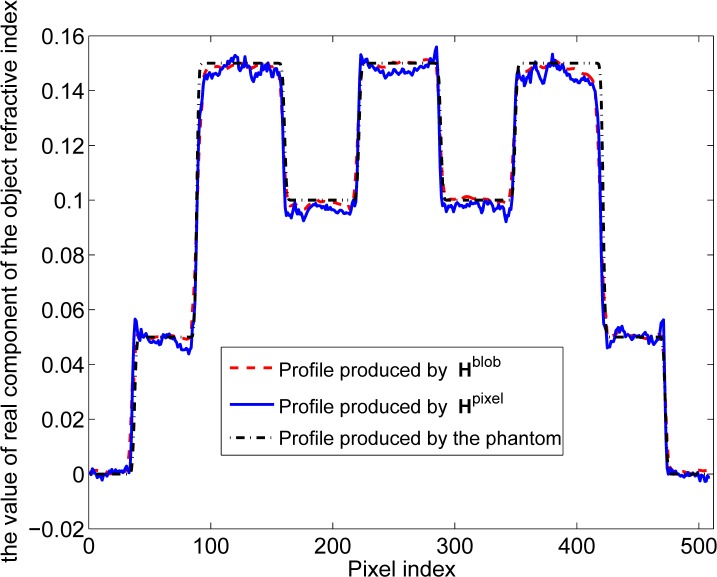
Computer-simulation studies were conducted to validate our reconstruction algorithm implementations that utilized the system matrices H^pixel and H^blob. Example images reconstructed from noisy data sets by use of H^pixel and H^blob are shown in Figs. 8(a) and 8(b). The system matrix H^pixel utilized linear interpolation and H^blob utilized blob parameters relative radius a = 2, m = 2, and α = 10.4. The regularization parameter was set at γ = 10 for both cases. Horizontal profiles through the centers of the images in Figs. 8(a) and 8(b) are shown in Fig. 9. The solid blue line (pixel-based result) appears to overshoot some of the boundaries and has more oscillations than the dashed red line (blob-based result). Note that the grey levels of the true object were recovered with good fidelity due to the fact that the object was contained within the field-of-view of the simulated imaging system and therefore there was no truncation of the data function with respect to the detector coordinate.

Fig. 8.

Examples of reconstructed images by use of PLS algorithms based on pixel system matrix H^pixel and blob system matrix H^blob. Regularization parameter γ = 10 for both cases. (a) An reconstructed image produced by pixel system matrix with linear interpolation. (b) An reconstructed image produced by blobs with relative radius a = 2 (physical size 100μm), m = 2 and α = 10.4.

Fig. 9.

(Color online) Profiles through the center row of the reconstructed images in Fig. 8. The solid blue line corresponds to Fig. 8(a). The dashed red and dashdotted black lines correspond to Fig. 8(b) and the true phantom.

4.2.2. Empirical determination of image statistics and resolution measures

For each combination of system matrix and regularization parameter, the mean image and image variance were estimated [46] from the associated set of 100 noisy images within the 70×70 pixel region-of-interest (ROI) indicated by the white box in Fig. 7. The average value of the image variance map was computed to establish a scalar summary measure of the variance associated with the ROI. To quantify the spatial resolution, we fitted the profile in the mean image corresponding to the boundary indicated in Fig. 7. The profile was fit to a cumulative Gaussian function [47]:

$$G(x)=I_1+\genfrac{}{}{0.1ex}{}{I_2-I_1}{2}\left(1+\text{erf}(\genfrac{}{}{0.1ex}{}{x-\mu }{\sigma \sqrt{2}})\right),$$ (24)

where x denotes the coordinate along the image profile, I₁ and I₂ indicate the image values on the two sides of the boundary with I₁ < I₂, μ is the true boundary location, and erf(x) is the error function, and σ is the associated standard deviation. We adopted the full-width at half-maximum (FWHM) value of the fitted error function as a summary measure of spatial resolution [47] at that location in image space, with smaller values indicating higher spatial resolution. Repeating these procedures for different choices of the regularization parameter γ produced a collection of (variance, FWHM) pairs for each system matrix, which were plotted to characterize the trade-offs between spatial resolution and noise levels in the reconstructed images.

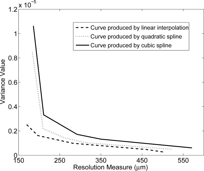
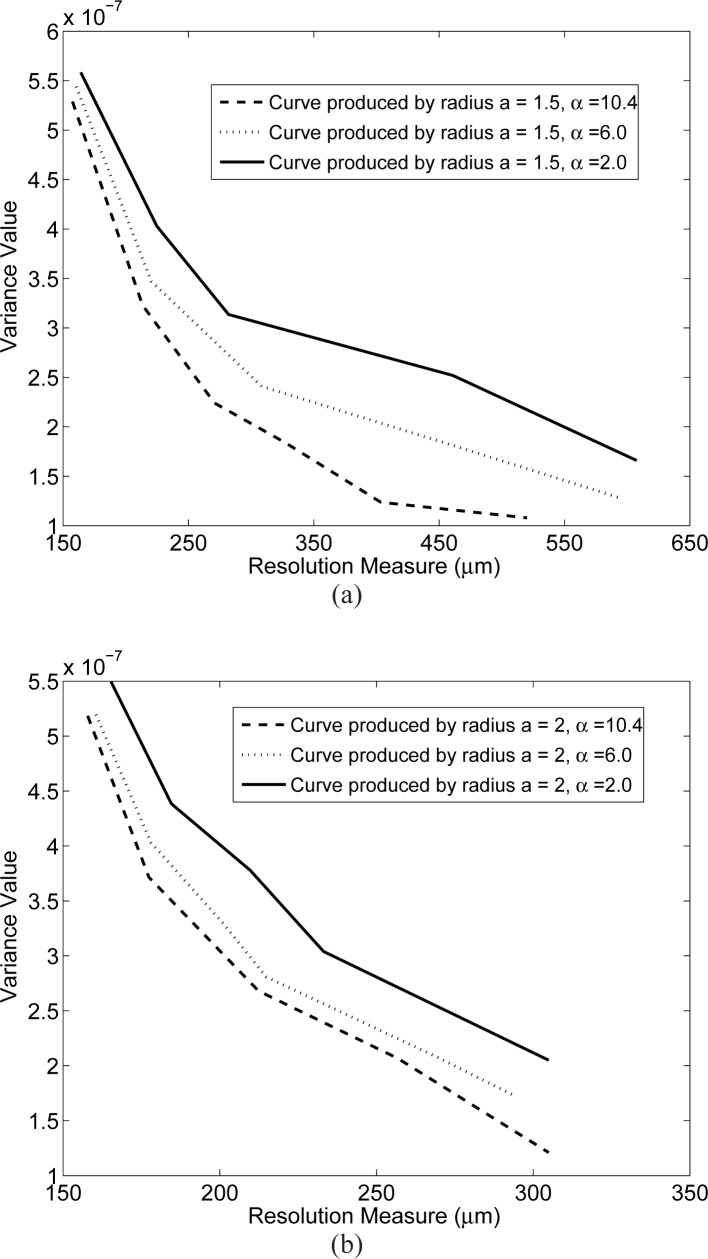
The variance-resolution curves for the pixel- and blob-based system matrices are shown in Figs. 10 and 11, respectively. The left-most point on each curve corresponds to γ = 10, while the right-most point on each curve corresponds to γ = 5000. As expected, when the value of γ increases, the image variance decreases at the cost of spatial resolution.

Fig. 10.

Variance versus resolution curves corresponding to use of the system matrices H^pixel.

Fig. 11.

Variance versus resolution curves corresponding to use of the system matrices H^blob. (a) Curves are produced by blobs with relative radius a = 1.5 (physical size 75μm), m = 2 and varying α. (b) Curves are produced by blobs with relative radius a = 2 (physical size 100μm), m = 2 and varying α.

For the pixel-based case, Fig. 10 reveals that the curve corresponding to the use of a linear weighting kernel is the lowest, followed by those corresponding to the quadratic and cubic spline kernels. Stated otherwise, the use of the linear interpolation-based system matrix H^pixel produced images with smaller variances at any of the attained spatial resolution values than did the other two system matrices. These observations are consistent with the singular value spectra displayed in Fig. 2, where the linear and cubic spline-based system matrices were demonstrated to yield the best and worst, respectively, conditioned system matrices for the pixel-based studies.

For the blob-based cases shown in Fig. 11, the variance-resolution curves corresponding to the shape parameter α = 10.4 were lower than those corresponding to the other α values for both relative radius a = 1.5 [Fig. 11(a)] and relative radius a = 2 [Fig. 11(b)]. The curves corresponding to the shape parameter α = 2.0 were higher than the others for both values of a. These observation are consistent with the singular value spectra displayed in Figs. 3 and 4, where the system matrices H^blob corresponding to α = 10.4 and α = 2.0 were demonstrated to yield the best and worst, respectively, conditioned system matrices for the blob-based studies.

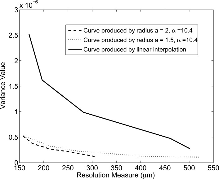
In order to facilitate the comparison of the pixel- and blob-based results, the three best variance-resolution curves from Figs. 10 and 11 were superimposed and replotted in Fig. 12. Two of these curves correspond to different H^blob with α = 10.4 and relative radius a = 1.5 and relative radius a = 2 and the third to H^pixel employing the linear weighting kernel. The two blob-based curves are everywhere lower than the pixel-based curve, indicating images produced by use of H^blob can possess improved variance-resolution trade offs than those produced by use of H^pixel. Below we demonstrate and investigate the use of H^blob for reconstructing images of biological tissue from few-view experimental differential projection data.

Fig. 12.

The three best variance-resolution curves picked from the pixel and blob cases.

5. Application to few-view image reconstruction

5.1. Experimental data and image reconstruction algorithm

In our studies of few-view image reconstruction, we utilized experimental DPCT data that were acquired previously [4] using a grating-based phase-contrast imaging system at the Swiss Light Source. A tissue sample corresponding to a rat brain was the imaged object. The tomographic scanning consisted of 720 tomographic view angles that were uniformly distributed over a 180 degree angular range. The differential projection data contained 1621 samples at each view angle corresponding to a detector pitch of 7μm. In the studies described below, certain subsets of these data were employed for few-view image reconstruction. A phase-stepping procedure was employed, which utilized four steps, to compute the differential projection data at each tomographic view angle. We refer the reader to reference [4] for additional details regarding the data-acquisition and sample preparation.

To obtain an estimate of the object function based on Eq. (20), the constrained, total variation minimization (TV) program [48–50] was employed:

$$\begin{array}{ccc}\multicolumn{1}{c}{\widehat{\mathbf{b}}=\underset{\mathbf{b}}{\text{arg}\hspace{0.17em}\text{min}}{\Vert \mathbf{b}\Vert }_{\text{TV}}}& \multicolumn{1}{c}{\text{s.t.}}& \multicolumn{1}{c}{\left|\mathbf{g}-{\mathbf{H}}^{\mathit{blob}}\mathbf{b}\right|\le \varepsilon ,}\end{array}$$ (25)

in which ||b||_TV represents the TV norm of the vector b and ɛ is the specified data tolerance. It has been demonstrated that this image reconstruction strategy can be highly effective at mitigating data-incompleteness for certain classes of objects [50–52]. The adaptive steepest-descent-projection onto convex sets (ASD-POCS) algorithm proposed by Sidky and Pan [51] was employed to determine approximate solutions of Eq. (25). Details regarding this algorithm and its implementation can be found in reference [51]. The system matrix H^blob with m = 2, relative radius a = 2 (physical size 14μm, which is twice the sampling interval 7μm) and α = 10.4 was constructed as described in Sec. 3.2. The values of the data tolerance ɛ employed were 43.8 and 58.2 for the reconstruction problems involving 90 and 180 view angles, respectively. From knowledge of b̂, estimates of δ_a(r₂; z) were obtained by use of Eq. (3) and were subsequently sampled by use of a 2D Dirac delta sampling function with a period of 7 μm onto a Cartesian grid for display. Because it is commonly employed in current applications of DPCT, we also reconstructed images by use of a modified FBP algorithm that acts directly on the differential projection data [11].

5.2. Reconstructed images

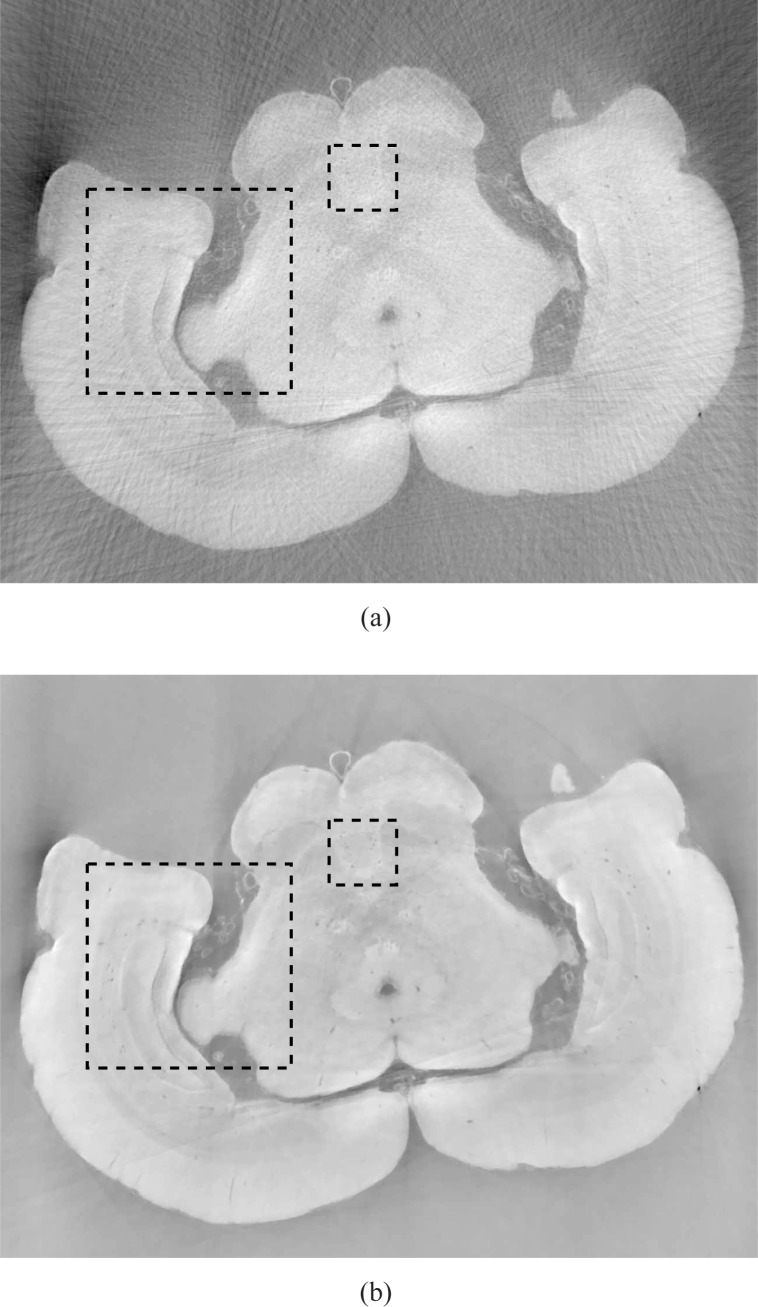
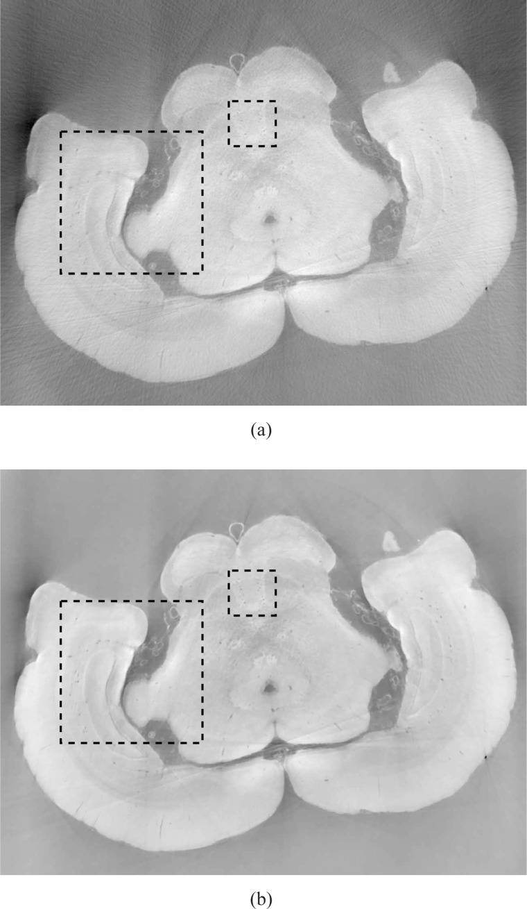
The images reconstructed by use of the FBP algorithm and the TV algorithm from 90 view angles are displayed in Figs. 13(a) and 13(b). The corresponding images reconstructed from 180 view angles are displayed in Fig. 14. All of the images are displayed in the same grey scale window. The images reconstructed by use of the FBP algorithm [Figs. 13(a) and 14(a)] have streak artifacts due to the limited number of view angles employed, while those artifacts are suppressed in the images reconstructed by use of the ASD-POCS algorithm [Figs. 13(b) and 14(b)]. Because the object was embedded in a container that did not fit entirely in the field-of-view, there was effectively projection truncation. Therefore, we expect that our reconstruction algorithm will reconstruct δ(r) only up to a constant. Because the true values of δ(r) were not available, we did not investigate this. All the images presented were normalized into the same scale.

Fig. 13.

Images reconstructed from 90 projections by use of the (a) FBP (b) ASD-POCS algorithm. The dashed boxes indicate two ROIs chosen for comparison. All images are displayed in the same grey scale window [0 1].

Fig. 14.

Images reconstructed from 180 projections by use of the (a) FBP (b) ASD-POCS algorithm Two dashed boxes indicate two ROIs chosen for comparison. All images are displayed in the same grey scale window [0 1].

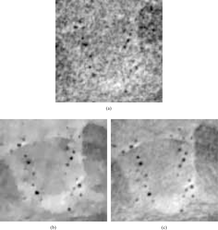
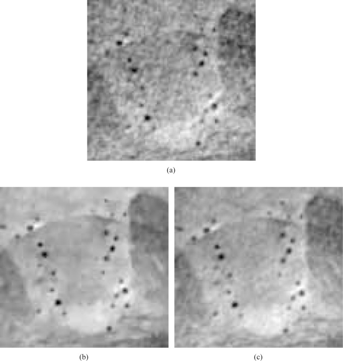
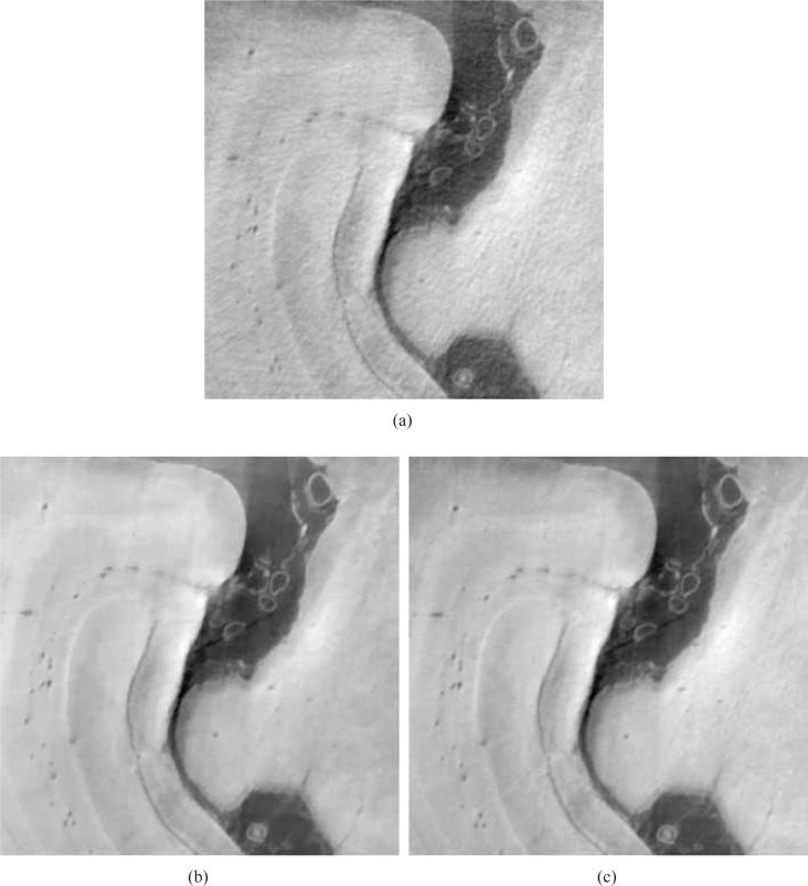
In order to more easily visualize differences in the reconstructed images, two ROIs indicated by black dashed boxes in Fig. 13(a) were displayed. Figures 15(a) and 15(b) display the smaller ROIs corresponding to images in Figs. 13(a) and 13(b), respectively, for the 90 view angle case. Subfigure (c) displays the smaller ROI extracted from an FBP image reconstructed from 720 view angles, which serves as a reference image. Figures 16(a) and 16(b) display the smaller ROIs corresponding to Figs. 14(a) and 14(b), respectively, for the 180 view angle case. Figure 16(c) displays the smaller ROI from the FBP reference image. As shown in Fig. 15(a) the visual appearance of the image reconstructed by use of the FBP algorithm from 90 projections is significantly degraded by noise and other artifacts. Some of the blood vessels (dark hole-like structures) may be difficult to detect due to the high artifact and noise levels in these image. The images reconstructed by use of the ASD-POCS algorithm from 90 tomographic views, shown in Figs. 15(b) has significantly reduced noise and artifact levels and possesses a visual appearance similar to the reference image that was reconstructed from the complete data set containing 720 views. Similar observations hold for the smaller ROI images corresponding to the 180 view angle case displayed in Fig. 16.

Fig. 15.

Zoomed-in images of the smaller ROIs denoted in Figs. 13(a) and (b), reconstructed from 90 view angles, are displayed in subfigures (a) and (b). Subfigure (c) displays the corresponding reference ROI corresponding to an image reconstructed from 720 projections by use of a DPCT FBP algorithm. All images are displayed in the same grey scale window [0 1].

Fig. 16.

Zoomed-in images of the smaller ROIs denoted in Figs. 14(a) and (b), reconstructed from 180 view angles, are displayed in subfigures (a) and (b). Subfigure (c) displays the corresponding reference ROI corresponding to an image reconstructed from 720 projections by use of a DPCT FBP algorithm. All images are displayed in the same grey scale window [0 1].

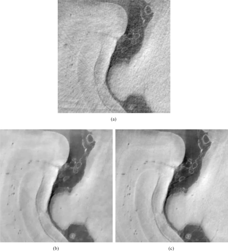
The larger ROIs are shown in Figs. 17 and 18. Figures 17(a) and 17(b) display the larger ROIs corresponding to images in Figs. 13(a) and 13(b), respectively, for the 90 view angle case. Subfigure (c) displays the larger ROI extracted from the FBP image reconstructed from 720 view angles, which again serves as a reference image. Figures 18(a) and 18(b) display the larger ROIs corresponding to images in Figs. 14(a) and 14(b), respectively, for the 180 view angle case. Subfigure (c) displays the larger ROI from the FBP reference image. Again, we observe that the images reconstructed by use of the ASD-POCS algorithm from 90 tomographic views, shown in Figs. 17(b) has significantly reduced noise and artifact levels and possesses a visual appearance similar to the reference image that was reconstructed from the complete data set containing 720 views. Similar observations hold for the larger ROI images corresponding to the 180 view angle case displayed in Fig. 18.

Fig. 17.

Zoomed-in images of the larger ROIs denoted in Figs. 13(a) and (b), reconstructed from 90 view angles, are displayed in subfigures (a) and (b). Subfigure (c) displays the corresponding reference ROI corresponding to an image reconstructed from 720 projections by use of a DPCT FBP algorithm. All images are displayed in the same grey scale window [0 1].

Fig. 18.

Zoomed-in images of the larger ROIs denoted in Figs. 14-(a) and (b), reconstructed from 180 view angles, are displayed in subfigures (a) and (b). Subfigure (c) displays the corresponding reference ROI corresponding to an image reconstructed from 720 projections by use of a DPCT FBP algorithm. All images are displayed in the same grey scale window [0 1].

6. Summary

We have analyzed the numerical and statistical properties of two classes of discrete imaging models that form the basis for iterative image reconstruction in DPCT. The models differ in the choice of expansion functions that were utilized to discretize the sought-after object function. The models based on Kaiser-Bessel window functions (“blobs”) were demonstrated to produced images that possess more favorable variance-resolution trade-offs than images reconstructed by use of pixel-based imaging models. This observation was consistent with the results of an SVD analysis of the system matrices, which demonstrated that the blob-based system matrices can yield more stable reconstruction problems than do pixel-based ones.

A reconstruction algorithm that seeks solutions of a constrained TV minimization optimization program was employed with a blob-based imaging model for few-view image reconstruction. By use of few-view experimental data, it was demonstrated that this algorithm can produce images with significantly weaker artifacts and lower noise levels than the FBP algorithm that has been utilized the majority of previously published studies. To our knowledge, this was the first published application of an iterative reconstruction method in X-ray DPCT for reconstruction of a biological specimen. We expect that the findings of our study will benefit the continued development of DPCT imaging systems by permitting reduction of data-acquisition times and radiation doses. Future research efforts will be required to identify blob parameters that are optimal for specific imaging tasks.

Appendix A: Explicit construction of the pixel-based system matrices

Below we describe how the matrices H^pixel employed in our numerical studies were constructed by use of Eq. (15). Specifically, because H^R is defined by Eq. (10) with the elements provided in reference [30], we need to specify the explicit forms of discrete derivative operator H^D for the three kernel functions W(x_r, d) employed.

A general form of the matrix H^D can be expressed as follows

$${\mathbf{H}}^{\mathbf{D}}=\left(\begin{array}{cccccc}\multicolumn{1}{c}{{\mathbf{H}}^{11}}& \multicolumn{1}{c}{0}& \multicolumn{1}{c}{0}& \multicolumn{1}{c}{\cdots }& \multicolumn{1}{c}{\cdots }& \multicolumn{1}{c}{0}\\ \multicolumn{1}{c}{0}& \multicolumn{1}{c}{{\mathbf{H}}^{22}}& \multicolumn{1}{c}{0}& \multicolumn{1}{c}{\cdots }& \multicolumn{1}{c}{\cdots }& \multicolumn{1}{c}{0}\\ \multicolumn{1}{c}{0}& \multicolumn{1}{c}{0}& \multicolumn{1}{c}{\ddots }& \multicolumn{1}{c}{\cdots }& \multicolumn{1}{c}{\cdots }& \multicolumn{1}{c}{0}\\ \multicolumn{1}{c}{⋮}& \multicolumn{1}{c}{}& \multicolumn{1}{c}{\cdots }& \multicolumn{1}{c}{{\mathbf{H}}^{tt}}& \multicolumn{1}{c}{⋮}& \multicolumn{1}{c}{0}\\ \multicolumn{1}{c}{⋮}& \multicolumn{1}{c}{}& \multicolumn{1}{c}{\cdots }& \multicolumn{1}{c}{}& \multicolumn{1}{c}{\ddots }& \multicolumn{1}{c}{0}\\ \multicolumn{1}{c}{0}& \multicolumn{1}{c}{0}& \multicolumn{1}{c}{\cdots }& \multicolumn{1}{c}{0}& \multicolumn{1}{c}{0}& \multicolumn{1}{c}{{\mathbf{H}}^{TT}}\end{array}\right),$$

where H^tt(t = 1, 2,··· ,T) is a S × S matrix, T is the total number of projection views and S is the number of sampled projection data at each view. Explicit forms of H^tt are determined by different interpolation kernels W(x_r, h). Three types of H^tt corresponding to three different kernels W(x_r, h) adopted in the paper are provided as follows:

Linear interpolation kernel

$${\mathbf{W}}_1(d,h)=n_d\{\begin{array}{ll}\multicolumn{1}{c}{1-s}& \multicolumn{1}{c}{0\le s<1,s=\genfrac{}{}{0.1ex}{}{\left|d\right|}{h},}\\ \multicolumn{1}{c}{0}& \multicolumn{1}{c}{s\ge 1,}\end{array}$$

where n_d is a normalization constant which is determined by the dimensionality and the smoothing length h. The value of h was set to 2 times the projection sampling interval, and n_d is equal to $\genfrac{}{}{0.1ex}{}{1}{h}$. The explicit form of H^tt corresponding to use of W₁(x_r, d) can be expressed as

$${\mathbf{H}}^{tt}={\left(\begin{array}{cccccc}\multicolumn{1}{c}{\cdots }& \multicolumn{1}{c}{\cdots }& \multicolumn{1}{c}{\text{boundary}}& \multicolumn{1}{c}{\text{condition}}& \multicolumn{1}{c}{\cdots }& \multicolumn{1}{c}{\cdots }\\ \multicolumn{1}{c}{-1/2}& \multicolumn{1}{c}{0}& \multicolumn{1}{c}{1/2}& \multicolumn{1}{c}{0}& \multicolumn{1}{c}{0}& \multicolumn{1}{c}{\cdots }\\ \multicolumn{1}{c}{0}& \multicolumn{1}{c}{-1/2}& \multicolumn{1}{c}{0}& \multicolumn{1}{c}{1/2}& \multicolumn{1}{c}{0}& \multicolumn{1}{c}{\cdots }\\ \multicolumn{1}{c}{\cdots }& \multicolumn{1}{c}{\ddots }& \multicolumn{1}{c}{\ddots }& \multicolumn{1}{c}{\cdots }& \multicolumn{1}{c}{\ddots }& \multicolumn{1}{c}{⋮}\\ \multicolumn{1}{c}{\cdots }& \multicolumn{1}{c}{\cdots }& \multicolumn{1}{c}{0}& \multicolumn{1}{c}{-1/2}& \multicolumn{1}{c}{0}& \multicolumn{1}{c}{1/2}\\ \multicolumn{1}{c}{\cdots }& \multicolumn{1}{c}{\cdots }& \multicolumn{1}{c}{\text{boundary}}& \multicolumn{1}{c}{\text{condition}}& \multicolumn{1}{c}{\cdots }& \multicolumn{1}{c}{\cdots }\end{array}\right)}_{S\times S},$$

where the the boundary condition elements are appropriately defined. In our studies, the projection data were not truncated and the object was embedded in uniform background medium. In this case, the boundary condition elements were set to zero.

Quadratic spline

$${\mathbf{W}}_2(d,h)=n_d\{\begin{array}{ll}\multicolumn{1}{c}{\genfrac{}{}{0.1ex}{}{3}{4}-s^2}& \multicolumn{1}{c}{0\le s<\genfrac{}{}{0.1ex}{}{1}{2},s=\genfrac{}{}{0.1ex}{}{\left|d\right|}{h},}\\ \multicolumn{1}{c}{\genfrac{}{}{0.1ex}{}{9}{8}-\genfrac{}{}{0.1ex}{}{3}{2}s+\genfrac{}{}{0.1ex}{}{s^2}{2}}& \multicolumn{1}{c}{\genfrac{}{}{0.1ex}{}{1}{2}\le s<\genfrac{}{}{0.1ex}{}{3}{2},}\\ \multicolumn{1}{c}{0}& \multicolumn{1}{c}{s\ge \genfrac{}{}{0.1ex}{}{3}{2},}\end{array}$$

where h was set to 2 times the projection sampling interval, and n_d is equal to $\genfrac{}{}{0.1ex}{}{1}{h}$. The explicit form of H^tt corresponding to use of W₂(x_r, d) can be expressed as

$${\mathbf{H}}^{tt}={\left(\begin{array}{cccccccc}\multicolumn{1}{c}{\cdots }& \multicolumn{1}{c}{\cdots }& \multicolumn{1}{c}{\cdots }& \multicolumn{1}{c}{\text{boundary}}& \multicolumn{1}{c}{\text{condition}}& \multicolumn{1}{c}{\cdots }& \multicolumn{1}{c}{\cdots }& \multicolumn{1}{c}{\cdots }\\ \multicolumn{1}{c}{-1/8}& \multicolumn{1}{c}{-1/4}& \multicolumn{1}{c}{0}& \multicolumn{1}{c}{1/4}& \multicolumn{1}{c}{1/8}& \multicolumn{1}{c}{0}& \multicolumn{1}{c}{\cdots }& \multicolumn{1}{c}{\cdots }\\ \multicolumn{1}{c}{0}& \multicolumn{1}{c}{-1/8}& \multicolumn{1}{c}{-1/4}& \multicolumn{1}{c}{0}& \multicolumn{1}{c}{1/4}& \multicolumn{1}{c}{1/8}& \multicolumn{1}{c}{0}& \multicolumn{1}{c}{\cdots }\\ \multicolumn{1}{c}{\cdots }& \multicolumn{1}{c}{\ddots }& \multicolumn{1}{c}{\ddots }& \multicolumn{1}{c}{\ddots }& \multicolumn{1}{c}{\ddots }& \multicolumn{1}{c}{\ddots }& \multicolumn{1}{c}{⋮}& \multicolumn{1}{c}{0}\\ \multicolumn{1}{c}{⋮}& \multicolumn{1}{c}{\ddots }& \multicolumn{1}{c}{0}& \multicolumn{1}{c}{-1/8}& \multicolumn{1}{c}{-1/4}& \multicolumn{1}{c}{0}& \multicolumn{1}{c}{1/4}& \multicolumn{1}{c}{1/8}\\ \multicolumn{1}{c}{\cdots }& \multicolumn{1}{c}{\cdots }& \multicolumn{1}{c}{\cdots }& \multicolumn{1}{c}{\text{boundary}}& \multicolumn{1}{c}{\text{condition}}& \multicolumn{1}{c}{\cdots }& \multicolumn{1}{c}{\cdots }& \multicolumn{1}{c}{\cdots }\end{array}\right)}_{S\times S}.$$

Cubic spline

$${\mathbf{W}}_3(d,h)=n_d\{\begin{array}{ll}\multicolumn{1}{c}{\genfrac{}{}{0.1ex}{}{2}{3}-s^2+\genfrac{}{}{0.1ex}{}{s^3}{2}}& \multicolumn{1}{c}{0\le s<1,s=\genfrac{}{}{0.1ex}{}{\left|d\right|}{h},}\\ \multicolumn{1}{c}{\genfrac{}{}{0.1ex}{}{4}{3}-2s+s^2-\genfrac{}{}{0.1ex}{}{s^3}{6}}& \multicolumn{1}{c}{1\le s<2,}\\ \multicolumn{1}{c}{0}& \multicolumn{1}{c}{s\ge 2,}\end{array}$$

where h was set to 2 times the sampling interval with linear interpolation case, and n_d is equal to $\genfrac{}{}{0.1ex}{}{1}{h}$. The explicit form of H^tt corresponding to use of W₃(x_r, d) can be expressed as

$${\mathbf{H}}^{tt}={\left(\begin{array}{cccccccccc}\multicolumn{1}{c}{\cdots }& \multicolumn{1}{c}{\cdots }& \multicolumn{1}{c}{\cdots }& \multicolumn{1}{c}{\cdots }& \multicolumn{1}{c}{\text{boundary}}& \multicolumn{1}{c}{\text{condition}}& \multicolumn{1}{c}{\cdots }& \multicolumn{1}{c}{\cdots }& \multicolumn{1}{c}{\cdots }& \multicolumn{1}{c}{\cdots }\\ \multicolumn{1}{c}{-1/32}& \multicolumn{1}{c}{-1/8}& \multicolumn{1}{c}{-5/32}& \multicolumn{1}{c}{0}& \multicolumn{1}{c}{5/32}& \multicolumn{1}{c}{1/8}& \multicolumn{1}{c}{1/32}& \multicolumn{1}{c}{0}& \multicolumn{1}{c}{\cdots }& \multicolumn{1}{c}{\cdots }\\ \multicolumn{1}{c}{0}& \multicolumn{1}{c}{-1/32}& \multicolumn{1}{c}{-1/8}& \multicolumn{1}{c}{-5/32}& \multicolumn{1}{c}{0}& \multicolumn{1}{c}{5/32}& \multicolumn{1}{c}{1/8}& \multicolumn{1}{c}{1/32}& \multicolumn{1}{c}{0}& \multicolumn{1}{c}{\cdots }\\ \multicolumn{1}{c}{⋮}& \multicolumn{1}{c}{\ddots }& \multicolumn{1}{c}{\ddots }& \multicolumn{1}{c}{\ddots }& \multicolumn{1}{c}{\ddots }& \multicolumn{1}{c}{\ddots }& \multicolumn{1}{c}{\ddots }& \multicolumn{1}{c}{\ddots }& \multicolumn{1}{c}{\cdots }& \multicolumn{1}{c}{⋮}\\ \multicolumn{1}{c}{0}& \multicolumn{1}{c}{\cdots }& \multicolumn{1}{c}{0}& \multicolumn{1}{c}{-1/32}& \multicolumn{1}{c}{-1/8}& \multicolumn{1}{c}{-5/32}& \multicolumn{1}{c}{0}& \multicolumn{1}{c}{5/32}& \multicolumn{1}{c}{1/8}& \multicolumn{1}{c}{1/32}\\ \multicolumn{1}{c}{\cdots }& \multicolumn{1}{c}{\cdots }& \multicolumn{1}{c}{\cdots }& \multicolumn{1}{c}{\cdots }& \multicolumn{1}{c}{\text{boundary}}& \multicolumn{1}{c}{\text{condition}}& \multicolumn{1}{c}{\cdots }& \multicolumn{1}{c}{\cdots }& \multicolumn{1}{c}{\cdots }& \multicolumn{1}{c}{\cdots }\end{array}\right)}_{S\times S}.$$

Appendix B: The derivation of the Eq. (18) in Sec.3.2

Let ξ ≡ x_r – x_n cosθ – y_n sinθ. As demonstrated by Lewitt [34], The 2D Radon transform of one window function is given by

$$\mathbf{R}{\varphi }_n^{\mathit{blob}}({\mathbf{r}}_2;m,a,\alpha )=\genfrac{}{}{0.1ex}{}{a}{I_m(\alpha )}{\left(\genfrac{}{}{0.1ex}{}{2\pi }{\alpha }\right)}^{1/2}{\left[\sqrt{1-{\left(\xi /a\right)}^2}\right]}^{m+1/2}{I}_{m+1/2}\left(\alpha \sqrt{1-{\left(\xi /a\right)}^2}\right),$$ (26)

for |ξ| ≤ a and zero otherwise. The gradient of the modified bessel function has the following relationship as [53]

$$\genfrac{}{}{0.1ex}{}{d}{dz}\left\{z^{\pm m}{I}_m(z)\right\}=z^{\pm m}{I}_{m\mp 1}(z),$$ (27)

where z is the distance to the center of the blob and m is a real number. Let $z=\alpha \sqrt{1-{\left(\xi /a\right)}^2}$. Note that Eqn. (26) can be re-expressed as

$$\mathbf{R}{\varphi }_n^{\mathit{blob}}({\mathbf{r}}_2;m,a,\alpha )=\genfrac{}{}{0.1ex}{}{a}{I_m(\alpha )}{\left(\genfrac{}{}{0.1ex}{}{2\pi }{\alpha }\right)}^{1/2}{\left(\genfrac{}{}{0.1ex}{}{1}{\alpha }\right)}^{m+1/2}{z}^{m+1/2}{I}_{m+1/2}(z).$$ (28)

By use of Eq. (27) and Eq. (28), along with the chain rule, it can be verified readily that

$$\begin{array}{ll}\multicolumn{1}{c}{\genfrac{}{}{0.1ex}{}{\partial \left(\mathbf{R}{\varphi }_n^{\mathit{blob}}(m,a,\alpha ,r)\right)}{\partial x_r}}& \multicolumn{1}{c}{=\genfrac{}{}{0.1ex}{}{\partial \left(\mathbf{R}{\varphi }_{\mathit{n}}^{\mathit{blob}}(m,a,\alpha ,r)\right)}{\partial z}\genfrac{}{}{0.1ex}{}{\partial z}{\partial \xi }\genfrac{}{}{0.1ex}{}{\partial \xi }{\partial x_r}}\\ \multicolumn{1}{c}{}& \multicolumn{1}{c}{=\genfrac{}{}{0.1ex}{}{a}{I_m[\alpha ]}{\left(\genfrac{}{}{0.1ex}{}{2\pi }{\alpha }\right)}^{1/2}{\left(\genfrac{}{}{0.1ex}{}{1}{\alpha }\right)}^{m+1/2}{z}^{m+1/2}{I}_{m-1/2}(z)\times {\left(\genfrac{}{}{0.1ex}{}{\alpha }{a}\right)}^2\left(-\genfrac{}{}{0.1ex}{}{\xi }{z}\right)}\\ \multicolumn{1}{c}{}& \multicolumn{1}{c}{=-\genfrac{}{}{0.1ex}{}{{\left(2\pi \alpha \right)}^{1/2}}{I_m(\alpha )}\genfrac{}{}{0.1ex}{}{\xi }{a}{\left(\sqrt{1-{\left(\xi /a\right)}^2}\right)}^{m-1/2}{I}_{m-1/2}\left(\alpha \sqrt{1-{\left(\xi /a\right)}^2}\right).}\end{array}$$ (29)