Ultrafast genome-wide scan for SNP–SNP interactions in common complex disease

Abstract

Long-range gene–gene interactions are biologically compelling models for disease genetics and can provide insights on relevant mechanisms and pathways. Despite considerable effort, rigorous interaction mapping in humans has remained prohibitively difficult due to computational and statistical limitations. We introduce a novel algorithmic approach to find long-range interactions in common diseases using a standard two-locus test that contrasts the linkage disequilibrium between SNPs in cases and controls. Our ultrafast method overcomes the computational burden of a genome × genome scan by using a novel randomization technique that requires 10× to 100× fewer tests than a brute-force approach. By sampling small groups of cases and highlighting combinations of alleles carried by all individuals in the group, this algorithm drastically trims the universe of combinations while simultaneously guaranteeing that all statistically significant pairs are reported. Our implementation can comprehensively scan large data sets (2K cases, 3K controls, 500K SNPs) to find all candidate pairwise interactions (LD-contrast ) in a few hours—a task that typically took days or weeks to complete by methods running on equivalent desktop computers. We applied our method to the Wellcome Trust bipolar disorder data and found a significant interaction between SNPs located within genes encoding two calcium channel subunits: RYR2 on chr1q43 and CACNA2D4 on chr12p13 (LD-contrast test, ). We replicated this pattern of interchromosomal LD between the genes in a separate bipolar data set from the GAIN project, demonstrating an example of gene–gene interaction that plays a role in the largely uncharted genetic landscape of bipolar disorder.

Genome-wide association studies (GWAS) have successfully identified hundreds of genetic markers associated with a wide range of diseases and quantitative traits (Hindorff et al. 2009; Manolio et al. 2009). Unfortunately, for most common diseases, nearly all associated variants have small effect sizes and taken together explain very little of the genetically heritable variation of the phenotype (Craddock 2007)—a phenomenon often posed as the conundrum of “missing heritability” (Maher 2008). Furthermore, single-locus association methods tend to implicate individual genes in a particular disease or trait, which in turn highlight a single biological entity involved (Saunders et al. 1993; Hugot et al. 2001; Neale et al. 2010). They do not, by definition, seek to implicate links between the functional elements of a system or elucidate pathway connections that may be broken. Investigation of joint gene–gene effects can therefore improve the explanatory ability of genetics twofold. Firstly, interaction—or statistical epistasis, as defined by Fisher (1918)—is hypothesized to explain a part of disease heritability (Marchini et al. 2005; Evans et al. 2006). Secondly, finding significant statistical links (epistatic or otherwise) between genes could provide strong indications of molecular-level interactions that differ between cases and controls.

However, an all-pairs (or all-triples) scan of SNPs genome-wide still poses widely discussed computational challenges due to the sheer size of the combinatorial space (Marchini et al. 2005), both for data sets typed on genotyping arrays ( SNPs) and sequencing technologies ( SNVs). Some methods address this problem by restricting the analysis to a small subset of candidate markers—those identified through single-locus analysis or those of biological interest (Emily et al. 2009), or by only checking for interactions between SNPs that are physically close to one another (Slavin et al. 2011). Others like EPIBLASTER (Kam-Thong et al. 2010) and SHIsisEPI (Hu et al. 2010) make use of specialized hardware like multiple Graphical Processing Units (GPUs) to finish computation on genome-wide data sets on the order of days, rather than weeks or months. While it is known that reductionist, candidate SNP-based approaches can miss many real interactions (Culverhouse et al. 2002; Evans et al. 2006) and fail to provide novel biological insights in an unbiased manner, brute-force approaches that rely on hardware for speedup may also scale poorly as data sets increase in size and interaction tests increase in complexity.

For genome-wide interaction analysis to become pervasive, there is a pressing need for algorithmic insights that make interaction testing on large data sets a scalable proposition, without placing undue computing or hardware demands on the investigator. The contribution of our work is such a method. Recently, others had exploited the fact that contrasting the linkage disequilibrium (Zhao et al. 2006), Pearson correlation (Kam-Thong et al. 2010) and log-odds ratio (Plink “--fast-epistasis” option) between a pair of SNPs in cases and controls could be computed more efficiently than maximum likelihood estimates in a logistic regression. Usefully, these computationally efficient contrast tests showed high congruence with statistical epistasis under a variety of genetic models. In this study, we do not devise a new statistical test; rather, we use a simplified version of the LD-contrast test for interaction (Zhao et al. 2006) to demonstrate our computational principles. Our version seeks pairs of physically unlinked (often interchromosomal) SNPs that are in strong LD in cases, but in weak LD, no LD, or reverse LD in controls.2

Our computational approach is driven by the intuition that most genome-wide interaction methodologies only report SNP pairs that are statistically significant (as per the test used) after correcting for the number of tests. The question we ask is this: Given a statistical test, is it possible to identify all the significant SNP pairs with high probability (power), without actually applying the test to all possible combinations genome-wide? In other words, can we design a search algorithm that accepts an arbitrary significance cutoff (as input from the user), and then finds all SNP pairs that will pass this cutoff without a brute-force search? We show here that for some contrast tests, this is indeed possible. At this juncture, it is imperative that we point out the two distinct meanings of “power”: Here, unless otherwise specified, we mean the power of an algorithm to identify SNP pairs for which a test statistic is large (i.e., significant), whereas in the broader context of genome-wide interaction mapping literature, power is the ability of a statistical test to detect a real interaction in the data set. Our work focuses on addressing the computational issues that plague an exhaustive search for interaction, leaving issues of statistical power for a separate discussion.

The rest of this study is structured as follows. First, we briefly review a simple LD-contrast test that compares LD between binary allelic states (rather than 0/1/2 genotypes) in cases and controls. Next, we present a novel computational framework—probably approximately complete (PAC) testing—that quantifies the power of a search done by an algorithm. PAC is an intuitive concept: For example, a brute-force method that tests all-pairs of SNPs genome-wide is considered fully powered at finding all significant pairs in our framework (i.e., 100% probability of finding all pairs whose test statistic clears the significance cutoff) and have no element of approximation at all (i.e., 100% complete scan of the interaction space in the case-control data set). In this study, we design a two-stage PAC test for common complex diseases that is guaranteed to find all significant pairwise interactions with high power (e.g., probability >95% of finding all pairs with a significant statistic) by looking at almost the entire space of possibilities (e.g., ∼99% complete scan of interaction space). In return for accepting a small loss of certainty and power, we show that algorithms that offer tremendous computational gains can be designed. We evaluate the performance of our implementation of this framework (SIXPAC) on genome-scale data and then present the results of our analysis on bipolar disorder (BD) in the Wellcome Trust Case Control Consortium (WTCCC) data set (Craddock 2007).

Methods

Outline

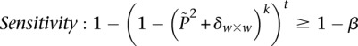
The goal of our method is to efficiently identify the set of SNP pairs that have vastly different LD in cases and controls from the universe of pairs genome-wide—if any such pairs exist at all. First, we define the LD-contrast statistic and establish a minimum cutoff value that determines whether a pair of SNPs has a statistically significant contrast in a genome-wide study or not. Next, we devise a stage 1 filtering step that identifies potential case–control differences in LD by looking for LD in cases alone. We quantify the losses that stage 1 incurs (false negatives) by applying this “approximate” version of the full LD-contrast test.

In stage 2, the candidates shortlisted based on their LD in cases are tested using the full cases-versus-controls LD-contrast test and either validated or discarded based on the difference. Stage 2 is needed to distinguish stage 1 shortlisted candidates that are true interactions from false positives. False positives may include SNP pairs drawn by pure chance, and also pairs that show large LD in cases, but also show large LD in controls in the same direction. Such a systemic inflation of disequilibrium between alleles in cases and controls might be due to other factors like population stratification, technical artifacts, or ascertainment bias and is, by definition, not associated with phenotype.

The motivation for dividing the search into two stages is because the stage 1, case-only, “approximate” filtering step can be processed extremely rapidly by exploiting computer bitwise operations, making it much faster than a brute-force approach. We present the novel randomization technique called group-sampling with which we can efficiently find SNP pairs that are in strong LD in cases. However, like every randomization algorithm, we need to stop sampling when we are reasonably certain that all significant (high LD) candidates have already been encountered and shortlisted. Consequently, at the end of stage 1, we are left with a “probably complete” list of pairs that demonstrate severe LD in cases. Taken in conjunction, this design outputs a “probably approximately complete” (PAC) catalog of interacting SNP pairs at the end of the filtering stage, which are subsequently screened by the full test. We demonstrate that our software implementation of this PAC-testing framework can find approximately all significant SNP pairs in current GWAS data sets with arbitrarily high power (e.g., >99% probability) at a fraction of the computational cost of an exhaustive search.

Definitions and notation

For purposes of illustration, consider two binary matrices and , representing the cohorts of haploid cases and haploid controls typed at polymorphic sites, respectively (we extend this to the diploid human case below). denotes the allele carried by case at variant site (0 for major, 1 for minor), while similarly denotes the allele carried of control at that site. Furthermore, we respectively denote and 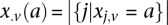as the number of cases and controls that carry allele at . 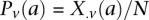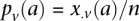Therefore, and are the corresponding allele -frequencies of in cases and controls. Since we are only discussing binary carrier states , for ease of notation, we henceforth use instead of , and ( instead of (and analogously, and for controls).

We are interested in examining whether a haploid individual carries a certain combination of alleles at two (or more) sites. Consider different binary sites , at which an individual can carry any one of unique allelic combinations. We say an individual carries allelic state 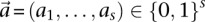at these sites if she carries allele at each one of the respective sites . Analogous to individual sites, we can also denote the different -frequencies of by 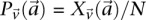in cases and 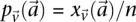in controls, where and are the number of carriers at in cases and controls, respectively. For example, if an individual carries 1-alleles (i.e., minor alleles) at each of the sites , then we say she is a -carrier of . The -frequency of in cases (controls) is the fraction of cases (controls) that are -carriers of .

Binary representation of diploid genomes

For diploid genomes like humans, equivalent matrices of cohorts would be for cases and for controls, where each entry in these matrices represents the number of minor alleles at the site, rather than the presence or absence of a minor allele. Depending on the model of interaction the investigator is interested in, these may be transformed into an appropriate binary representation in several ways. For our purpose, we represent each ternary genotype as two binary variables. The first variable asks whether the individual carries copies of the minor allele (i.e., is dominant) at this SNP, while the second asks whether the individual carries exactly copies of the minor allele (i.e., is recessive) at this SNP. In this format, cases and controls are represented by the binary matrices and , respectively, where each genotype is recoded as two binary values for cases,

and is recoded equivalently as for controls. For example, case #6 is represented as a recessive carrier of SNP #12 (variable coordinates: row 6, column by setting . If case #6 is a dominant carrier of SNP #12, then we set both and . The notations for number of carriers and frequency of variables (and combination of variables) all follow analogously.

Statistical test for two-locus effect

We adapt the LD-contrast test for interaction between a pair of unlinked genotypes (Zhao et al. 2006) into a similar two-tailed test between a pair of unlinked binary variables ,

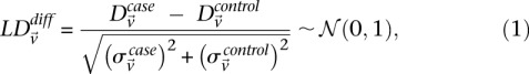where and represent the estimated LD between these variables in cases and controls, respectively, while and represent the standard error of these estimators (see Supplemental Section 1 for derivation and details) and is their LD contrast. This normalized statistic behaves as a Z-score, and for variable pairs that pass the significance cutoff in a genome-wide pairwise analysis (typically or less on present day data sets), this statistic will assume large values (typically 6 or more).

Variable pairs with large differences in LD are of interest to several genetic models, and their signal can be dissected to reveal either statistical (epistatic) or biological interaction. Based on what is known about the genetic architecture of a specific disease, the relevant community of geneticists can bring different model assumptions to bear on a test for interaction. Here, we do not attempt to dictate a specific model that might cause such a difference in LD between the cases and controls. Rather, we focus on presenting a general method that can report all SNP pairs with a significant contrast and provide expert users with the flexibility to filter the results from such an analysis according to relevant assumptions. This can be done either a priori (e.g., removing SNPs with marginal signals before running a search for interaction), or a posteriori (e.g., discarding reported SNP pairs that do not provide evidence for statistical epistasis).

Two-stage testing design

A widely used simplification (Piegorsch et al. 1994; Yang et al. 1999; Cordell 2009) in genome-wide interaction scans is to divide the search effort into two stages: first filter candidates, and then verify interaction. The crucial insight that permits this step is that we can expect physically unlinked markers to be in (or almost in) linkage equilibrium in large outbred populations. Even for common diseases, the general population is mostly composed of healthy controls (disease prevalence <50%). We show that in the absence of confounding factors like population stratification, a pair of physically unlinked variables showing large LD contrast will be a pair that has large LD in cases rather than large LD in controls. Without loss of generality, we focus our discussion on identifying pairs with strong positive LD in cases 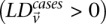. Pairs with strong negative LD between variables are easily modeled (with a trivial change in binary encoding) as strong positive LD between the major allele at one and a minor allele at the other. Alternative variable pairings of this kind would only require a different binary encoding scheme but introduce more confusing notation. A separate (but limiting) issue is that of the statistical testing burden incurred by encoding alternate models, which we address in the Discussion.

A sequential two-stage testing strategy is designed as follows.

Stage 1 (shortlisting)

The stage 1 null hypothesis states that any pair of distal variables should be in linkage equilibrium in cases.

From Equation S1.1 (see Supplemental Section 1), we know that the distribution of is . We shortlist only those variable pairs that reject the stage 1 null hypothesis at a significance level of . In other words, for a pair to be shortlisted as a candidate for follow-up, we require that the LD in cases between its variables should exceed some threshold, i.e., . We determine this threshold to satisfy sensitivity/specificity constraints below.

Stage 2 (validating)

Next, we apply the LD-contrast test on candidates shortlisted by stage 1. This helps us to determine, for each candidate, whether the observed LD is indeed case-specific (and therefore a putative indicator of interaction) or pervasive in the population (and hence unrelated to disease). The stage 2 null hypothesis posits that there is no LD difference between cases and controls:

Putative significant pairs will reject this null hypothesis at a significance level of (i.e., ).

To appreciate how such a two-stage design can capture almost all significant pairs in the data set and what the appropriate significance cutoff in the stage 1 analysis must be, we now introduce the concept of a probably approximately complete search. A numerical example depicting the concepts that follow is provided in Supplemental Section 9.

Probably approximately complete (PAC) search

Complete search

To find all significant variable pairs in the data set, current algorithms would sequentially visit each pair of SNPs, genome-wide, and check whether each LD contrast exceeds the user-prescribed significance threshold by comparing cases and controls.

Approximately complete search

Here we ask, what threshold can we apply in the filtering step, so as to capture almost all significant pairs by means of their disequilibrium in cases alone? In other words, can most significant pairs (pairs for which ) be captured without explicitly determining at all? Furthermore, we wish to determine the proportion of significant pairs that such an approximation might miss. We show that for most common diseases, an adequate cutoff for LD in cases is usually (see Supplemental Section 2)—i.e. SNP-pairs with a severe LD-contrast (difference in LD between cases and controls) are usually observable from their severe LD in cases alone.

Probably approximately complete (PAC) search

So far, our two-stage design has reduced the cumbersome task of counting the number of carriers for all variable pairs (genome-wide) in cases and then again in controls, to the simpler task of shortlisting the small set of pairs that demonstrate . From a complexity standpoint, however, such a simplification (restricting the stage 1 analysis to cases only) does not change the order or magnitude of the number of tests: This is still quadratic in the number of SNPs genome-wide. To address this computational problem, we now introduce the novel randomization technique called “group sampling,” which can rapidly perform the case-only shortlisting with arbitrarily high power, without explicitly checking all pairs of variables.

Group sampling

Rationale

From our observation that the LD statistic in cases is usually more severe than LD contrast (Supplemental Section 2), we deduce that significant interacting pairs will show a minimum number of excess -carriers in cases: . In a genome-wide analysis, as the universe of variable pairs tested grows, so does the burden of multiple test correction that is applied to characterize statistical significance. Consequently, the number of excess of -carriers required in order for to achieve statistical significance in cases——grows commensurately. Group sampling overcomes the computational burden of a genome-wide analysis by using this “side effect” of multiple-test correction to its advantage: The larger the number of variants typed, the larger is the universe of pairs to be tested, and the larger the excess -carriers needed to make statistically significant pairs stand apart from the crowd. This observation allows us to quickly prune the universe of pairs into a much smaller candidate set that is “guaranteed” to contain all significant pairs with arbitrarily high probability.

For illustration purposes, let us consider a simplified version of the problem at hand. In this version, we are only interested in searching through pairs of distal variables , where both variables have 1-frequencies ( and ) that lie within the narrow frequency window . Let the set of all variables that lie within this frequency window be labeled . We wish to determine whether there exists a pair , such that rejects . We can compute a lower bound on for all such as:

This is because the excess -carriers required for any 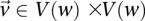to reject is at least as many as the excess -carriers required by the least frequent in that set: when . Therefore, the -frequency of all pairs that reject is at least:

where is the minimum LD in cases for all significant pairs .

Sampling a single group

Consider a group of cases drawn randomly (with replacement). If rejects , then the probability that all cases in the group will be -carriers of has a lower bound . On the contrary, if does not reject , then the probability that such a group will contain all -carriers of purely by chance has an upper bound 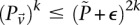—corresponding to the most frequent variable pair in . It is easy to see that if , we are much more likely to observe a random group of cases that are all -carriers of when it rejects .

The reason for drawing cases in groups (as opposed to one by one) is that it allows us to rapidly find the subset of variables for which all cases are -carriers. This is done with a native bitwise AND operation using computers, which is very fast in practice. In fact, the larger the group size, the exponentially smaller the subset of variables carried by all cases in the group becomes. Furthermore, long stretches of binary genotype data can be processed per CPU clock cycle, making this step even more attractive. Subsequent to finding this small subset of variables, it is computationally efficient to enumerate all pairs (or indeed, triplets) among them, and pass them on to stage 2.

Sampling multiple groups

If the group of cases we draw is sufficiently large (i.e., is high), then it is extremely unlikely to contain only -carriers, not only when accepts , but also when this null is rejected because both . We can counter this by drawing up to independent groups (each containing random cases), so that the probabilities of not witnessing even a single group containing only -carriers decreases at diverging rates for the two realities:

In fact, if does reject , then by varying the two parameters and the probability of observing at least one group of all -carriers can be driven arbitrarily high (type II error rate <) while keeping the probability of a chance observation relatively low (type I error rate <). In other words, given fixed specificity and sensitivity constraints and (provided as input by the user), when , we can always find group-sampling parameter values and for which:

An illustration to visualize this technique is provided in Figure 1, while the simple algorithm implied by our toy problem logic is provided by Algorithm 1. The general formulation for PAC testing across all frequency windows (genome-wide) is described in Supplemental Section 4 and the logic provided by Algorithm 2.

Figure 1.

Group sampling. A cohort of cases is shown on the left, where the cases outlined in red—, , , and —harbor an interacting pair of recessive variables. In other words, more cases carry the recessive–recessive combination than would be expected by chance, given the marginal frequencies of each recessive allele. By repeatedly drawing random groups of cases (here ), we are guaranteed to have drawn at least one group of individuals that carries both the variables in attempts with probability . These variables (and others) are quickly determined by a bitwise-AND operation between the group of cases. Then, all pairs of cocarried variables are enumerated and tested against the stage 1 null hypothesis (case-only analysis). Rejected combinations are shortlisted and followed up in stage 2 (case vs. control analysis), where an interaction is identified.

Algorithm 1. Group sampling toy problem.

Given all variables within frequency range

Calculate significance threshold

Calculate sampling parameters and

Repeat times:

Randomly choose a group of cases ( rows from )

Cocarried variables

For all unique combinations :

If do

Algorithm 2. Group sampling genome-wide (SIXPAC).

Assign all variables genome-wide to frequency windows

For every pair of windows :

Calculate significance threshold

Calculate sampling parameters and

Repeat times:

Randomly choose group of cases

Cocarried variables

Identify variables

Identify variables

For all unique combinations :

If do

For all shortlisted variables :

If output as an interaction

This concludes our discussion of a probably approximately complete search. PAC testing offers a powerful computational framework: As we shall demonstrate next, we can find approximately all significant SNP pairs genome-wide with high power in a fraction of the time that an exhaustive search would require.

Results

The major methodological contribution of this work is a novel randomization algorithm (group sampling), which can focus the computational effort toward finding significant pairwise interaction candidates, without testing all pairs genome-wide. To determine whether a candidate SNP pair is significant or not and to minimize the risk of false positives, in all our analyses, we subject the results to the most conservative threshold for significance in a genome-wide analysis—the Bonferroni corrected P-value of 0.05—unless otherwise stated. More sophisticated treatment of the multiple testing issues in interaction testing (e.g., Emily et al. 2009) is equally applicable and can be plugged into our method without violating any of the principles or assumptions. We also restrict our analysis to pairs of genetic markers (SNPs) only and choose to ignore gene–environment interactions for the moment. These simplifications serve to highlight the fundamental concepts of our approach, without loss of interpretable results. Our software implementation of this algorithm (SIXPAC) is available for download at http://www.cs.columbia.edu/∼snehitp/sixpac.

Data set

SIXPAC was used to analyze 1868 cases of the bipolar disorder (BD) cohort in the WTCCC against combined controls from the 1958 British birth cohort (58C) and UK national blood service (NBS), all typed on the Affymetrix 5.0 platform, after cleaning all data as per requirement (Craddock 2007). Each of the remaining 455,566 SNPs remaining in the data set was encoded into two binary variables (dominant and recessive), giving 911,132 binary variables genome-wide and a universe of potential variable pairs to be tested. Although we only report pairwise interactions that are significant at the Bonferroni level in this data set , investigators who use less stringent multiple test correction can use SIXPAC to discover interactions at a different cutoff as well.

To verify that the LD-contrast statistic follows a standard normal distribution, we drew random variable pairs genome-wide and constructed a QQ plot. Like others before (Liu et al. 2011), we observed that WTCCC data cleaning was inadequate for interaction analysis and systematically applied more stringent filters to preemptively screen out false positives that can be a result of bad genotype calls on a few individuals. Specifically, 81,085 additional SNPs that had <95% confidence calls (CHIAMO) in >1% of the individuals (cases and controls combined) were removed. For the cleaned data set of 374,481 SNPs that remain, we verified that the LD-contrast statistic for randomly drawn pairs of unlinked variables >5 cM apart was indeed a Z-score (QQ plots and additional cleaning details in Supplemental Section 5), in agreement with our null hypothesis.

Power analysis on spiked data

Next, we tested SIXPAC's computational sensitivity by searching for synthetic interactions inserted into the bipolar cases while keeping the joint controls unchanged. Eleven recessive–recessive interaction pairs between 22 SNPs on successive autosomal chromosomes (chr1 and chr2, chr3 and chr4, etc.) were simulated over a range of different parameters. Interactions between each pair of SNPs were simulated in a manner not to introduce a main effect, but effectively introduce only interaction effects. Details of this procedure are outlined in Supplemental Section 6.

Algorithm 2 configures the search parameters according to two user inputs: (1) a significance cutoff (LD-contrast test P-value), and (2) the minimum search power (defined as the power to discover all variable pairs that exceed the given significance cutoff, assuming such interactions exist). We tested SIXPAC on the synthetic data sets over a range of different input value combinations, to check whether we could discover the spiked interactions in accordance with theoretical estimates, and confirmed finding all of them at (or above) the power guaranteed to the user (Supplemental Section 7).

Figure 2.

Computational efficiency. Our implementation of the two-stage PAC-testing framework (SIXPAC, orange line) was benchmarked on the cleaned WTCCC bipolar disorder data set (approximately 2K cases, 3K controls, 450K SNPs, four genetic models tested per distal SNP pair, 400 billion pairwise tests genome-wide). (A) The factor reduction in the universe of SNP pairs achieved by stage 1, for each power setting. Note that unlike brute force, this does not mean down-sampling the universe of SNP pairs, but rather involves reducing the probability of identifying any one of them. For example, a brute-force method would presumably test 40 billion pairs (and ignore the remaining 360 billion) to achieve 10% power on this data set. However, PAC testing scans all 400 billion pairs, but simply reduces the probability of finding the significant interactions among them to 10%. This results in shortlisting ∼68× fewer combinations through stage 1. (B) The efficiency of our software implementation of this method. We compare the performance of SIXPAC against the time taken by a brute-force approach of applying the LD-contrast test directly to all pairs (green line). All tests were benchmarked on a common desktop computer configuration (Intel i7 quad-core processor, 2.67 GHz with 8 GB RAM). The last data point shows the 90% power benchmarks, followed by dotted lines that illustrate how these estimates may continue as we approach 100% power. SIXPAC, like any randomization algorithm, will require infinite compute time to achieve 100% power but can approach very close at a small fraction of the brute-force cost. Lastly, we note that these measurements only reflect the performance of our Java program rather than what might be feasible with a different implementation of the algorithm.

Computational savings from group sampling

To put the computational savings of our novel approach in context, we reviewed the literature for published, high-performance, genome-wide pairwise search methodologies that either (i) contrast a statistic for a pair of SNPs between cases and controls or (ii) directly test for statistical epistasis between a pair of SNPs using a regression model. Plink (Purcell et al. 2007) offers a --fast-epistasis option that tests pairs of SNPs using a statistic similar to ours: Specifically, it collapses each pair of SNPs completely into a 2×2 table of major versus minor allele counts, and subsequently contrasts the odds ratios of each combination between cases and controls. On the other hand, EPIBLASTER (Kam-Thong et al. 2010) operates on the entire 3×3 table of genotypes to contrast the exact Pearson's correlation of each SNP pair between cases and controls. Like Plink, SHEsisEPI (Hu et al. 2010) also contrasts odds-ratios of all SNP pairs reduced to a 2×2 table. Both EPIBLASTER and SHEsisEPI achieve speedup through the use of a GPU stack.

Among the methods that directly test for statistical epistasis, we report TEAM (Zhang et al. 2010a) and FastEpistasis (Schüpbach et al. 2010). The authors of FastCHI (Zhang et al. 2009), FastANOVA (Zhang et al. 2008), COE (Zhang et al. 2010b) and TEAM presented a review (Zhang et al. 2011) in which TEAM was reported as the most appropriate for handling human data sets, and was therefore chosen to represent the family of methods. TEAM achieves computational speedup by a novel approach that allows it to accurately identify interacting SNP pairs (for most statistical tests) by checking only a small subset of individuals in the cohort. Unlike EPIBLASTER, Plink --fast-epistasis, and SIXPAC, TEAM works directly on the logistic regression framework—giving it the ability to test a broader range of interaction models. The other method, FastEpistasis, reports epistasis in the analysis of quantitative traits (and is particularly built for gene-expression analysis) by implementing a rapid linear regression that takes advantage of multicore processor architectures. Notable among methods omitted in this comparison are Multifactor Dimensionality Reduction (Ritchie et al. 2001) and the Restricted Partition Method (Culverhouse et al. 2004), both of which partition the data according to genotypic effect in a relatively model agnostic manner. Consequently both methods test a variety of interaction models (alternate parameterizations) that are not currently captured by high-performance computational techniques like ours and others previously discussed. Another widely cited method, BEAM (Zhang and Liu 2007), does not scale to present day data sets (Cordell 2009) and was left out of this analysis. There are numerous other methods that perform whole-genome interaction scans (Emily et al. 2009; Zhang et al. 2009; Greene et al. 2010; Liu et al. 2011), including some that utilize sampling subsets of individuals for computational speedup (Achlioptas et al. 2011). An older review of a few of these is provided elsewhere (Cordell 2009).

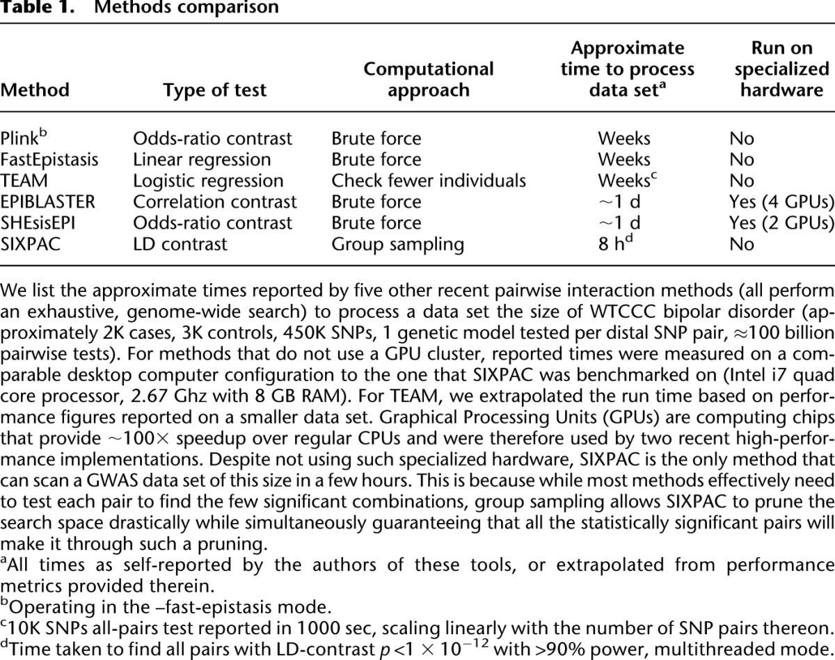
Except for SIXPAC, all the time scales presented in Table 1 are performance figures as self-reported by the authors of each method (or in the case of TEAM, extrapolated from performance figures reported therein) on a data set of this size. Our synopsis does not constitute a comprehensive methods comparison and is presented solely to highlight the computational savings achieved by group sampling (Fig. 2). The reason SIXPAC is able to achieve its speedup without GPUs is because it does not need to exhaustively test all pairs of SNPs to identify the significant combinations.3 On the other hand, all other methods are burdened by a brute-force test of all pairs to identify such combinations. In confirmation of our estimates, they also report that genome-wide testing on ordinary CPUs requires several weeks of compute time (some report weeks even on a small cluster of computers). The application of group sampling was able to reduce this computational investment to ∼8 h.

Table 1.

Methods comparison

Novel significant interaction in bipolar disorder

We ran SIXPAC on the BD data set with >95% power to check whether there exist any significant LD contrasts between pairs of physically unlinked variables (SNPs >5 cM apart). We report the presence of only one statistically significant two-locus contrast (BD cases vs. NBS+58C controls LD contrast, ) between SNPs lying within two calcium channel genes: rs10925490 within RYR2 on chr1q43, and rs2041140 and rs2041141 within CACNA2D4 on chr12p13.33. We successfully replicated the signal from this region at Bonferroni significance levels in a different bipolar data set of Europeans (653 BARD cases, 1034 GRU controls) from the GAIN initiative (The GAIN Collaborative Research Group 2007; Smith et al. 2009) (also see http://www.genome.gov/19518664), which were typed on a different platform (Affymetrix 6.0). Deeper investigation revealed that the SNP in CACNA2D4 is 200 kb away from CACNA1C—a known calcium channel gene whose association to BD was only recently confirmed by combining large GWAS data sets for meta-analyses (Ferreira et al. 2008; Sklar et al. 2008). Functional experiments have also confirmed the role played by genes at this locus in bipolar disorder (Perrier et al. 2011). Although channel ideopathies (and, more specifically, faults in calcium channels and signaling) have long been known to play a major role in bipolar disorder, single-locus association methods were underpowered to implicate genes in these pathways without considerably boosting their sample sizes (Craddock 2007; Ferreira et al. 2008; Sklar et al. 2008). Neither gene that we report—either at the known locus or novel locus—was identified as a candidate by the original WTCCC analysis (Craddock 2007), which focused on effects visible to single-locus association.

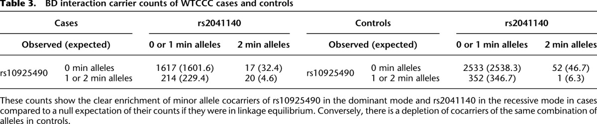
Specifically, we found that the dominance variable of rs10925490 (one or more minor alleles) was in severe positive linkage disequilibrium with the recessive variables of adjacent SNPs rs2041140 and rs2041141 (two minor alleles each) in BD cases, and slight negative disequilibrium with them in controls, giving an LD-contrast . To verify that this signal was not due to any unaccounted biases, we first confirmed that high LD between the two variables was specific to BD cases only, even when contrasted against samples from all other WTCCC disease phenotypes (six tests of BD vs. other-disease-cases all show LD-contrast ). Next, we performed a permutation analysis to characterize the empirical distribution of the LD-contrasts statistic at the theoretical significance level of (i.e., to check if 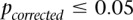). We ran SIXPAC on 100 phenotype permuted versions of the same data set (i.e., 100 whole-genome, all-pairs scans for interaction) and observed 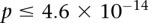between a pair of SNPs in only one such permutation ().

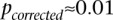Finally, we sought to replicate the observed difference in LD at these loci. In the GAIN data set, we considered all LD contrasts in an area of SNP immediately upstream and downstream of rs10925490 in the dominant allelic mode, against SNP immediately upstream and downstream of rs2041140 in the recessive allelic mode. In other words, we tested pairs (around and including the original interaction), to test if any pair in this area bore an LD contrast that passed the conservative Bonferroni significance cutoff . This roughly translates to a region kb upstream and downstream of each SNP in the original pair. Although there was no appreciable difference in LD between the same SNPs (rs2041140/rs10925490 shows LD-contrast ), we observed a significant LD contrast between rs2041140 and rs677730 (the SNP immediately upstream of rs10925490 on the Affymetrix 6.0 platform). To confirm that this observation was not likely by chance, we randomly picked 5000 pairs of physically unlinked (>5 cM apart) SNPs genome-wide and tested an equal neighborhood of LD contrasts around each pair in the GAIN data set. Only one out of 5000 random areas contained a SNP pair with a more significant LD contrast .

To get a better picture of the LD-contrast landscape between SNPs in this region, we conducted a wider survey of the area spanning SNPs (upstream, downstream, and including both rs2041140 and rs10925490) . The scan reveals several additional pairs of SNPs that show differences in LD going in the same direction (strong LD in cases, weak negative LD in controls), arranged in a strikingly similar pattern in both data sets, presenting strong evidence of an interlocus effect. The two-dimensional LD-contrast spectrum for this larger area is presented in Figure 3, alongside the Manhattan plots for marginal association at each locus. The top SNP pair in the area (rs677730, d × rs11062012, r) had LD-contrast in GAIN: A similar phenotype permutation analysis as earlier reveals that only 19 out of the 5000 randomly chosen areas genome-wide contained a more significant pair . It can also be seen that there is no marginally significant association at these loci in either data set. Table 2 and Table 3 present a summary of these results.

Figure 3.

Bipolar disorder interaction. In a genome-wide scan of all 400 billion variable pairs (four genetic models tested per SNP pair) in the WTCCC bipolar disorder data set (Affymetrix 500K), SIXPAC found one significant interaction between SNPs >5 cM apart that satisfied all our filtering criteria. The SNPs rs10925490 and rs2041140 lie within the RYR2 gene on chr1q43 and the CACNA2D4 gene on chr12p13.33, respectively. Each figure shows the −log(P-value) from a standard single-locus association test (allelic model) of the two SNPs as well as 25 SNPs immediately upstream and downstream from each of them, along the x-axis and y-axis. Also shown in the grayscale area is the −log(p) from the pairwise LD-contrast test of all variable pairs. As suggested by the original finding, SNPs around rs10925490 were considered in dominant allelic mode, while SNPs around rs2041140 were in recessive mode. We replicated this signal by similarly testing dominant–recessive pairs of variables around the very same SNPs in a much smaller bipolar disorder data set from the GAIN Consortium (Affymetrix 6.0). In the replication data set, we observe several pairs that cross the significance threshold and a strikingly similar visual pattern in the LD-contrast landscape (see main text for a permutation analysis). The top pair (rs677730–rs11062012) in this area is pinpointed with dashed lines (see main text for permutation analysis). Standard single-locus association analysis does not yield any significant result in either data set, as seen in the marginal Manhattan plots (the gray dashed line represents the genome-wide significance level).

Table 2.

Bipolar disorder interaction

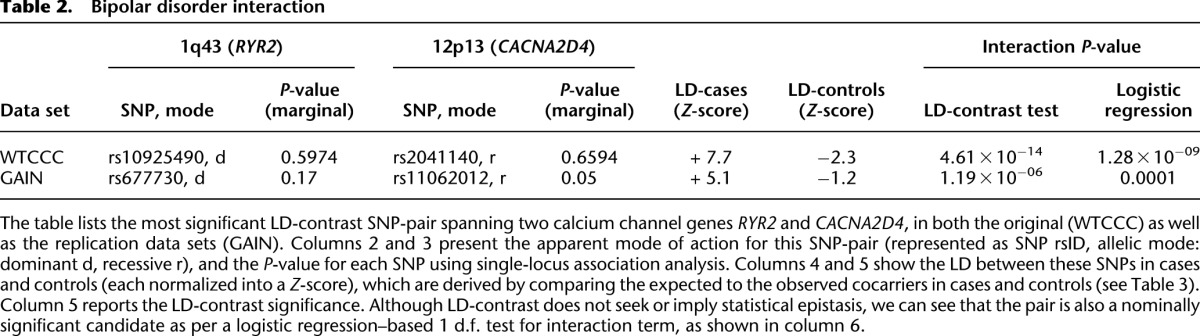
Table 3.

BD interaction carrier counts of WTCCC cases and controls

Discussion

In this study, we introduced a novel method that defuses the computational challenge of a genome × genome interaction scan by using the statistical constraint toward, rather than against, our goal. Focusing only on interactions that have a chance of achieving statistically significant association, we developed a rapid filter that does not require the naive arduous scan of all pairs of variants. To demonstrate its utility, we implemented an established test for interaction that contrasts LD between cases and controls, to demonstrate how an exhaustive genome-wide multilocus association search is possible while saving an order of magnitude or more in computational resources. Usefully, we are also able to provide performance guarantees and quantify the approximate nature of our output, and our algorithm brings genome-wide three-locus scans into the realm of feasibility.

While the focus of this contribution is computational methodology, we prove applicability in practice to a classical GWAS data set. Among widely investigated common diseases, bipolar disorder remains one of the most recalcitrant phenotypes to GWAS methodology (Craddock and Sklar 2009), perhaps in part because of the limitations of single-locus association analysis. We highlight the power and utility of multilocus effects in terms of uncovering molecular processes by exposing two calcium channel–coding genes as affecting bipolar disorder, supporting recent discoveries that were only made possible through a significant increase in data set size. We have replicated this observation in an independent data set, strongly suggesting a bona fide underlying interaction between members of a gene family known to be functionally associated with bipolar disorder, making it suitable for further investigation.

Compared to the number of single-locus associations, GWAS of common phenotypes in humans have uncovered very few reproducible gene–gene effects so far. This is partly because interaction analyses for human populations are difficult to design and interpret (Cordell 2002; Phillips 2008). A conventional test for statistical epistasis is expected to only identify loci whose combined effect on phenotype is not explained by the addition of their individual effects, for an appropriately chosen scale. In case–control studies, this typically involves applying a logistic regression to check for significance of the interaction term(s) after accounting for main effects (Wang et al. 2010), which is equivalent to a test for deviation from multiplicative odds (or additive log-odds). However, there are several limitations to this approach—scale of choice (Mani et al. 2008), assumption of a genetic model by which two loci combine their effects (Hallander and Waldmann 2007), limited models of interaction that can be tested (Li and Reich 1999; Hallgrímsdóttir and Yuster 2008), and limited sensitivity of logistic regression to non-normal residuals, among others. How these factors might cumulatively affect a test for other models of genetic interaction has not yet been decisively established.

Furthermore, true biological interaction between two or more loci may or may not manifest itself as a departure from additivity. Two loci whose main effects appear to combine in an additive manner might also indicate their biological co-involvement (and hence “interaction”) underlying the disease (Wang et al. 2011). In general, two-locus association tests are known to contribute signal independently from what is seen by conventional single-locus association tests (Marchini et al. 2005; Kim et al. 2010), and comprehensive multilocus association strategies may be worth undertaking despite the increased multiple testing burden (Evans et al. 2006). Indeed, recent work (Zuk et al. 2012) showing that alternative models of biological interaction could confound estimates of heritability has redirected the attention of the genetics community to the potential of interaction studies.

A previous genome-wide scan for statistical epistasis on the same bipolar disorder data set had reported Bonferroni significant epistasis between rs10124883 and four other SNPs (Hu et al. 2010). As expected, all four pairs approached (but did not clear) Bonferroni significance levels as per the LD-contrast test as well —and could therefore be captured simply by lowering the significance cutoff. This congruence between tests for statistical epistasis and contrast tests has been exploited by others (Plink, EPIBLASTER) and, indeed, also holds for the binary LD-contrast test (see tables in Supplemental Section 6). But whereas other methods would use a brute-force testing strategy to identify candidate SNP pairs, PAC testing will accomplish the same result much quicker by looking at a small fraction of the pairs.

Our findings do suggest that unlike stepwise regression approaches that sequentially attribute residual variance/deviance to each of their components, tests that make fewer assumptions regarding scale may, indeed, be more powerful at capturing a wider range of interactions. Conversely, a distinct advantage of regression over our LD-contrast test remains its clear interpretation and measurement of effect size; although the difference in LD between cases and controls is consistent and reproducible across data sets, it does not immediately suggest a clear causal genetic model underlying this signal. We dissected this interaction using the standard logistic regression, , where codes for dominance carrier status at rs10925490 while codes for recessive carrier status at rs2041140. The main effects were observed to be not significant, while the epistasis term was considerable (), suggesting deviation from multiplicative odds is one option. We also considered the standard full genotype model (0/1/2 parameterization of predictor variables) with 8 degrees of freedom (Cordell and Clayton 2002) as implemented by INTERSNP (Herold et al. 2009), where the most significant test (Test 6, ) was the one comparing the full model against a model that accounts for just within-SNP additive and dominance effects. In a genome-wide search for interaction using logistic regression, these levels are likely to fall short of significance cutoffs after correcting for hundreds of billions of tests performed, which explains why other methods seeking statistical epistasis on the same BD data set did not report LD between the RYR2-CACNA2D4 as a significant finding. A true etiological understanding of this persistent difference in LD may require sequencing at each locus to identify the interacting variants.

Limitations and extensions

The major contribution of this work is a computational technique to rapidly identify SNP pairs with large values of a test statistic without performing a brute-force search. While we assessed the issue of power with regard to our randomization algorithm, we left the separate (but equally important) concept of statistical power unaddressed—i.e., the ability of an interaction test to spot a true biological interaction in the data set. Although contrasting LD, correlation, and odds-ratios between cases and controls have all separately been characterized as powerful tests for interaction, each test makes specific model assumptions and is powerful only under its own regime. Consequently, the absence of interaction reported by SIXPAC (or, indeed, by any other software) does not imply the absence of interaction itself, but could simply mean lack of statistical power of the test, inadequate number of samples, or, simply, incorrect model assumptions. During the course of publishing this method, minor corrections were suggested for a range of contrast statistics to improve their power and decrease type I error rate (Ueki and Cordell 2012). Again, we note that modifications to these tests can be easily adopted into our computational methods—which are agnostic of statistics.

In contrast to the performance gains offered by group sampling are its two notable weaknesses. First—like any other randomization algorithm—group sampling can never achieve 100% power (probability of completion), whereas brute-force approaches will. Second, by virtue of limiting itself to binary features, testing for genetic models that incorporate allelic dosage and trend effects using group sampling does not appear straightforward. Although extending our computational principles to implement rapid correlation and odds-ratio contrast tests (among others) may be appealing, the loss of statistical power from increasing the number of tests is less easily addressed. Where we currently encode recessive and dominance binary status, each additional test may require a different encoding of features (genotypes, or combinations thereof), thereby adding to the multiple testing burden. Overcoming these limitations appears nontrivial, and increases in sample size will almost certainly play a crucial role in discovering these hidden genetic connections.

Extrapolating from the hardware speedups reported by others (Hu et al. 2010; Kam-Thong et al. 2010) may suggest that a high-performance GPU-enabled implementation of our method might offer a scan of all-pairwise interactions in a few minutes, and all three-way interactions on the order of a day(s) in large GWAS data sets. But a more immediate concern related to testing three-way interactions would be the statistical power and semantic interpretation of such a test (conceivably devised on a 2×2×2 binary table). In conclusion, we note that while the transition of association studies from SNP arrays to full ascertainment of variants may have led to analytical emphasis on rarer alleles, it has only increased the impetus to examine the spectrum of multilocus effects. With so many more variants to consider, the computational limitations will only become more severe, but the solutions reported will be ever more essential.

References

- Achlioptas P, Schölkopf B, Borgwardt KM 2011. Two-locus association mapping in subquadratic runtime. Proceedings of the 17th ACM SIGKDD conference on knowledge discovery and data mining, August 21–24, 2011, San Diego, CA, USA. Association for Computing Machinery, New York [Google Scholar]
- Cordell HJ 2002. Epistasis: What it means, what it doesn't mean, and statistical methods to detect it in humans. Hum Mol Genet 11: 2463–2468 [DOI] [PubMed] [Google Scholar]
- Cordell HJ 2009. Detecting gene–gene interactions that underlie human diseases. Nat Rev Genet 10: 392–404 [DOI] [PMC free article] [PubMed] [Google Scholar]
- Cordell HJ, Clayton DG 2002. A unified stepwise regression procedure for evaluating the relative effects of polymorphisms within a gene using case/control or family data: Application to HLA in type 1 diabetes. Am J Hum Genet 70: 124–141 [DOI] [PMC free article] [PubMed] [Google Scholar]
- Craddock N 2007. Genome-wide association study of 14,000 cases of seven common diseases and 3,000 shared controls. Nature 447: 661–678 [DOI] [PMC free article] [PubMed] [Google Scholar]
- Craddock N, Sklar P 2009. Genetics of bipolar disorder: Successful start to a long journey. Trends in Genetics 25: 99–105 [DOI] [PubMed] [Google Scholar]
- Culverhouse R, Suarez BK, Lin J, Reich T 2002. A perspective on epistasis: Limits of models displaying no main effect. Am J Hum Genet 70: 461–471 [DOI] [PMC free article] [PubMed] [Google Scholar]
- Culverhouse R, Klein T, Shannon W 2004. Detecting epistatic interactions contributing to quantitative traits. Genet Epidemiol 27: 141–152 [DOI] [PubMed] [Google Scholar]
- Emily M, Mailund T, Hein J, Schauser L, Schierup MH 2009. Using biological networks to search for interacting loci in genome-wide association studies. Eur J Hum Genet 17: 1231–1240 [DOI] [PMC free article] [PubMed] [Google Scholar]
- Evans DM, Marchini J, Morris AP, Cardon LR 2006. Two-stage two-locus models in genome-wide association. PLoS Genetics 2: e157 doi: 10.1371/journal.pgen.0020157 [DOI] [PMC free article] [PubMed] [Google Scholar]
- Ferreira MA, O'Donovan MC, Meng YA, Jones IR, Ruderfer DM, Jones L, Fan J, Kirov G, Perlis RH, Green EK, et al. 2008. Collaborative genome-wide association analysis supports a role for ANK3 and CACNA1C in bipolar disorder. Nature Genetics 40: 1056–1058 [DOI] [PMC free article] [PubMed] [Google Scholar]
- Fisher RA 1918. On the correlation between relatives on the supposition of Mendelian inheritance. Trans R Soc Edinb 52: 399–433 [Google Scholar]
- The GAIN Collaborative Research Group 2007. New models of collaboration in genome-wide association studies: The Genetic Association Information Network. Nat Genet 39: 1045–1051 [DOI] [PubMed] [Google Scholar]
- Greene CS, Sinnott-Armstrong NA, Himmelstein DS, Park PJ, Moore JH, Harris BT 2010. Multifactor dimensionality reduction for graphics processing units enables genome-wide testing of epistasis in sporadic ALS. Bioinformatics 26: 694–695 [DOI] [PMC free article] [PubMed] [Google Scholar]
- Hallander J, Waldmann P 2007. The effect of non-additive genetic interactions on selection in multi-locus genetic models. Heredity 98: 349–359 [DOI] [PubMed] [Google Scholar]
- Hallgrímsdóttir IB, Yuster DS 2008. A complete classification of epistatic two-locus models. BMC Genet 9: 17 doi: 10.1186/1471-2156-9-17 [DOI] [PMC free article] [PubMed] [Google Scholar]
- Herold C, Steffens M, Brockschmidt FF, Baur MP, Becker T 2009. INTERSNP: Genome-wide interaction analysis guided by a priori information. Bioinformatics 25: 3275–3281 [DOI] [PubMed] [Google Scholar]
- Hindorff LA, Sethupathy P, Junkins HA, Ramos EM, Mehta JP, Collins FS, Manolio TA 2009. Potential etiologic and functional implications of genome-wide association loci for human diseases and traits. Proc Natl Acad Sci 106: 9362–9367 [DOI] [PMC free article] [PubMed] [Google Scholar]
- Hu X, Liu Q, Zhang Z, Li Z, Wang S, He L, Shi Y 2010. SHEsisEpi, a GPU-enhanced genome-wide SNP–SNP interaction scanning algorithm, efficiently reveals the risk genetic epistasis in bipolar disorder. Cell Research 20: 854–857 [DOI] [PubMed] [Google Scholar]
- Hugot JP, Chamaillard M, Zouali H, Lesage S, Cézard JP, Belaiche J, Almer S, Tysk C, O'Morain CA, Gassull M, et al. 2001. Association of NOD2 leucine-rich repeat variants with susceptibility to Crohn's disease. Nature 411: 599–603 [DOI] [PubMed] [Google Scholar]
- Kam-Thong T, Czamara D, Tsuda K, Borgwardt K, Lewis CM, Erhardt-Lehmann A, Hemmer B, Rieckmann P, Daake M, Weber F, et al. 2010. EPIBLASTER-fast exhaustive two-locus epistasis detection strategy using graphical processing units. Eur J Hum Genet 19: 465–471 [DOI] [PMC free article] [PubMed] [Google Scholar]
- Kim S, Morris NJ, Won S, Elston RC 2010. Single-marker and two-marker association tests for unphased case-control genotype data, with a power comparison. Genet Epidemiol 34: 67–77 [DOI] [PMC free article] [PubMed] [Google Scholar]
- Li W, Reich J 1999. A complete enumeration and classification of two-locus disease models. Hum Hered 50: 334–349 [DOI] [PubMed] [Google Scholar]
- Liu Y, Xu H, Chen S, Chen X, Zhang Z, Zhu Z, Qin X, Hu L, Zhu J, Zhao GP, et al. 2011. Genome-wide interaction-based association analysis identified multiple new susceptibility loci for common diseases. PLoS Genetics 7: 16 doi: 10.1371/journal.pgen.1001338 [DOI] [PMC free article] [PubMed] [Google Scholar]
- Maher B 2008. Personal genomes: The case of the missing heritability. Nature 456: 18–21 [DOI] [PubMed] [Google Scholar]
- Mani R, St Onge RP, Hartman JL, Giaever G, Roth FP 2008. Defining genetic interaction. Proc Natl Acad Sci 105: 3461–3466 [DOI] [PMC free article] [PubMed] [Google Scholar]
- Manolio TA, Collins FS, Cox NJ, Goldstein DB, Hindorff LA, Hunter DJ, McCarthy MI, Ramos EM, Cardon Lon R, Chakravarti A, et al. 2009. Finding the missing heritability of complex diseases. Nature 461: 747–753 [DOI] [PMC free article] [PubMed] [Google Scholar]
- Marchini J, Donnelly P, Cardon LR 2005. Genome-wide strategies for detecting multiple loci that influence complex diseases. Nat Genet 37: 413–417 [DOI] [PubMed] [Google Scholar]
- Neale BM, Fagerness J, Reynolds R, Sobrin L, Parker M, Raychaudhuri S, Tan PL, Oh EC, Merriam JE, Souied E, et al. 2010. Genome-wide association study of advanced age-related macular degeneration identifies a role of the hepatic lipase gene (LIPC). Proc Natl Acad Sci 107: 7395–7400 [DOI] [PMC free article] [PubMed] [Google Scholar]
- Perrier E, Pompei F, Ruberto G, Vassos E, Collier D, Frangou S 2011. Initial evidence for the role of CACNA1C on subcortical brain morphology in patients with bipolar disorder. Eur Psychiatry 26: 135–137 [DOI] [PubMed] [Google Scholar]
- Phillips PC 2008. Epistasis—the essential role of gene interactions in the structure and evolution of genetic systems. Nat Rev Genet 9: 855–867 doi: 10.1038/nrg2452 [DOI] [PMC free article] [PubMed] [Google Scholar]
- Piegorsch WW, Weinberg CR, Taylor JA 1994. Non-hierarchical logistic models and case-only designs for assessing susceptibility in population-based case-control studies. Stat Med 13: 153–162 [DOI] [PubMed] [Google Scholar]
- Purcell S, Neale B, Todd-Brown K, Thomas L, Ferreira M A R, Bender D, Maller J, Sklar P, De Bakker PIW, Daly MJ, et al. 2007. PLINK: A toolset for whole-genome association and population-based linkage analysis. Am J Hum Genet 81: 559–575 [DOI] [PMC free article] [PubMed] [Google Scholar]
- Ritchie MD, Hahn LW, Roodi N, Bailey LR, Dupont WD, Parl FF, Moore JH 2001. Multifactor-dimensionality reduction reveals high-order interactions among estrogen-metabolism genes in sporadic breast cancer. Am J Hum Genet 69: 138–147 [DOI] [PMC free article] [PubMed] [Google Scholar]
- Saunders AM, Strittmatter WJ, Schmechel D, George-Hyslop PHS, Pericak-Vance MA, Joo SH, Rosi BL, Gusella JF, Crapper-MacLachlan DR, Alberts MJ, et al. 1993. Association of apolipoprotein E allele ε4 with late-onset familial and sporadic Alzheimer's disease. Neurology 43: 1467–1472 [DOI] [PubMed] [Google Scholar]
- Schüpbach T, Xenarios I, Bergmann S, Kapur K 2010. FastEpistasis: A high performance computing solution for quantitative trait epistasis. Bioinformatics 26: 1468–1469 [DOI] [PMC free article] [PubMed] [Google Scholar]
- Sklar P, Smoller JW, Fan J, Ferreira MAR, Perlis RH, Chambert K, Nimgaonkar VL, McQueen MB, Faraone SV, Kirby A, et al. 2008. Whole-genome association study of bipolar disorder. Mol Psychiatry 13: 558–569 [DOI] [PMC free article] [PubMed] [Google Scholar]
- Slavin TP, Feng T, Schnell A, Zhu X, Elston RC 2011. Two-marker association tests yield new disease associations for coronary artery disease and hypertension. Hum Genet 130: 725–733 [DOI] [PMC free article] [PubMed] [Google Scholar]
- Smith EN, Bloss CS, Badner JA, Barrett T, Belmonte PL, Berrettini W, Byerley W, Coryell W, Craig D, Edenberg HJ, et al. 2009. Genome-wide association study of bipolar disorder in European American and African American individuals. Mol Psychiatry 14: 755–763 [DOI] [PMC free article] [PubMed] [Google Scholar]
- Ueki M, Cordell HJ 2012. Improved statistics for genome-wide interaction analysis. PLoS Genet 8: e1002625 doi: 10.1371/journal.pgen.1002625 [DOI] [PMC free article] [PubMed] [Google Scholar]
- Wang X, Elston RC, Zhu X 2010. The meaning of interaction. Hum Hered 70: 269–277 [DOI] [PMC free article] [PubMed] [Google Scholar]
- Wang X, Elston RC, Zhu X 2011. Statistical interaction in human genetics: How should we model it if we are looking for biological interaction? Nat Rev Genet 12: 74 doi: 10.1038/nrg2579-c2 [DOI] [PMC free article] [PubMed] [Google Scholar]
- Yang Q, Khoury MJ, Sun F, Flanders WD 1999. Case-only design to measure gene-gene interaction. Epidemiology 10: 167–170 [PubMed] [Google Scholar]
- Zhang Y, Liu JS 2007. Bayesian inference of epistatic interactions in case-control studies. Nat Genet 39: 1167–1173 [DOI] [PubMed] [Google Scholar]
- Zhang X, Zou F, Wang W 2008. FastANOVA: An efficient algorithm for genome-wide association study. KDD 3: 821–829 [PMC free article] [PubMed] [Google Scholar]
- Zhang X, Zou F, Wang W 2009. FastChi: An efficient algorithm for analyzing gene–gene interactions. Pac Symp Biocomput 2009: 528–539 [PMC free article] [PubMed] [Google Scholar]
- Zhang X, Huang S, Zou F, Wang W 2010a. TEAM: Efficient two-locus epistasis tests in human genome-wide association study. Bioinformatics 26: i217–i227 [DOI] [PMC free article] [PubMed] [Google Scholar]
- Zhang X, Pan F, Xie Y, Zou F, Wang W 2010b. COE: A general approach for efficient genome-wide two-locus epistasis test in disease association study. J Comput Biol 17: 401–415 [DOI] [PubMed] [Google Scholar]
- Zhang X, Huang S, Zou F, Wang W 2011. Tools for efficient epistasis detection in genome-wide association study. Source Code Biol Med 6: 1 doi: 10.1186/1751-0473-6-1 [DOI] [PMC free article] [PubMed] [Google Scholar]
- Zhao J, Jin L, Xiong M 2006. Test for interaction between two unlinked loci. Am J Hum Genet 79: 831–845 [DOI] [PMC free article] [PubMed] [Google Scholar]
- Zuk O, Hechter E, Sunyaev S, Lander E 2012. The mystery of missing heritability: Genetic interactions create phantom heritability. Proc Natl Acad Sci 109: 1193–1198 [DOI] [PMC free article] [PubMed] [Google Scholar]