

Abstract
Exceptionally accurate genome reference sequences have proven to be of great value to microbial researchers. Thus, to date, about 1800 bacterial genome assemblies have been “finished” at great expense with the aid of manual laboratory and computational processes that typically iterate over a period of months or even years. By applying a new laboratory design and new assembly algorithm to 16 samples, we demonstrate that assemblies exceeding finished quality can be obtained from whole-genome shotgun data and automated computation. Cost and time requirements are thus dramatically reduced.
Knowing the genome as exactly as possible is of fundamental value to microbial biology. Once thought to be impossible, de novo assembly of short, massively parallel sequencing data is now common practice, with several tools now available (e.g., Chaisson and Pevzner 2008; Zerbino and Birney 2008; MacCallum et al. 2009; Simpson et al. 2009; Li et al. 2010; Chapman et al. 2011; Gnerre et al. 2011; Simpson and Durbin 2012). Standard automated methods have yielded genome assemblies that are generally of good quality, and in a few cases, with some manual work, near-complete genomes have been achieved (Nagarajan et al. 2010; Rasko et al. 2011a). However, most assemblies have had many errors and gaps, both in the era of Sanger sequencing (Fraser et al. 2002) and in the current short read era (Klassen and Currie 2012). Importantly, the most difficult (e.g., rapidly evolving) regions are often absent or incorrectly rendered. Fortunately, bacteria have small genomes (generally 2–6 Mb), and thus in many cases, it has been feasible to expend extra effort to determine their sequences correctly. Indeed, to date, about 1800 bacterial genome assemblies (Genomes Online Database; http://www.genomesonline.org) (Kyrpides 1999), have gone through a process known as “finishing,” involving a combination of manual laboratory and computational processes (Chain et al. 2009). These processes are applied iteratively and are thus slow and expensive. There remains a need for new methods that are both faster and more economical.
To that end, in this study, we define a new recipe for whole-genome shotgun sequencing and a new algorithm to assemble such data, incorporated as part of the program ALLPATHS-LG (MacCallum et al. 2009). The recipe uses a mixture of three data types generated using sequencing technology from two vendors, Illumina (Bentley et al. 2008) and Pacific Biosciences (Eid et al. 2009), that together span a broad range in their resolving power. These technologies are complementary and, at least theoretically, provide the capability of accurately assembling the entire genome. All of the laboratory and computational methods are essentially automated, thus reducing costs and keeping project turnaround time to a minimum.
We apply these methods to 16 bacterial samples, three of which were previously finished, thus functioning as controls for our work. We applied the same laboratory methods and identical (pushbutton) computations to each of the resulting data sets. We describe the resulting assemblies (complete circles in several cases), and for those having the finished reference sequences are able to assess the accuracy both of our assemblies and the finished references rigorously.
Approach
Laboratory formula
We reasoned that creation of optimal assemblies would require both a new laboratory formula and a new algorithm, and that these would need to be synchronized. For our formula, we settled on three data types and approximate levels of coverage that could facilitate generation of assemblies of exceptionally high quality (Table 1; Grad et al. 2012; Supplemental Methods). In order of DNA size range, these data are (A) short fragment read pairs from Illumina, (B) long reads from Pacific Biosciences, and (C) jumping pairs from Illumina with a wide size range.
Table 1.
Laboratory formula for finished genome assembly
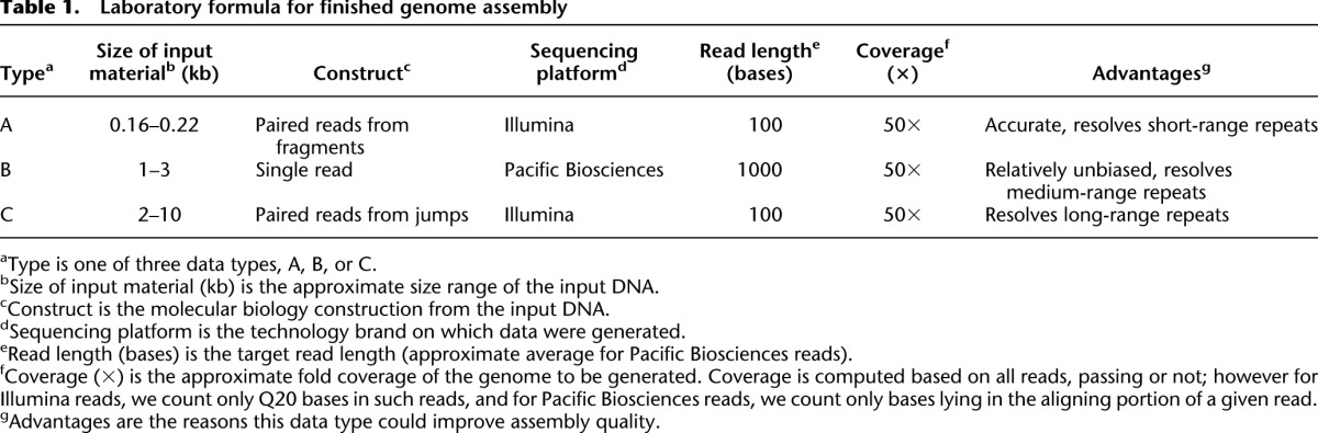
These data have complementary attributes. Thus, Illumina data have high base accuracy, compensating for the relatively low accuracy of the Pacific Biosciences data (Eid et al. 2009). Conversely, the Pacific Biosciences data are generated without amplification and thus could provide coverage in regions that are underrepresented or absent in Illumina data due to amplification bias in the sample preparation. Finally, the data are spread across three size ranges. In particular, we note that because the jumping pairs are created from a wide size range of material, they can span considerable distances (5 kb or more). However, there is a trade-off because a tight size range would give greater accuracy to distinguish shorter distances. Fortunately, the Pacific Biosciences reads are effective in the middle distance range where the jumps are not.
Assembly algorithm
A new algorithm was needed to exploit the relative strengths of the data types with respect to accuracy, bias, and resolution range. In outline, the algorithm proceeds roughly according to the following steps (for more detail, see Supplemental Methods; for explanatory diagrams, see Fig. 1):
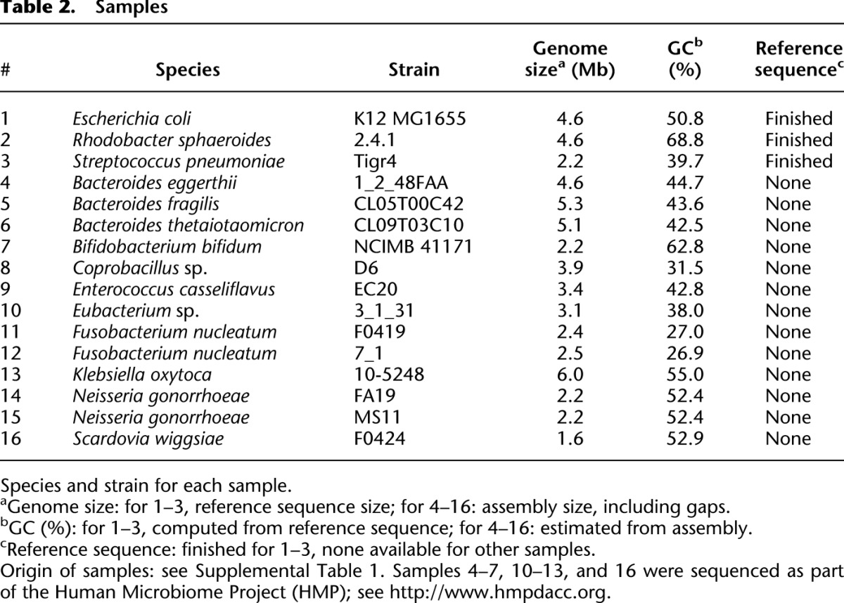
Figure 1.

Diagram of assembly method. (A) The ideal unipath graph depends on the genome and a constant K, the ‘minimum overlap.’ Perfect repeat copies of size K are ‘glued together.’ In the figure, this happens to two copies of a repeat R. (Unipath graphs are actually directed, and both strands of the genome must be accounted for, but we elide these points to facilitate exposition.) (B) As in main text Step I.1, starting from fragment read pairs (data type A), we construct an approximation to the ideal unipath graph. First, individual fragment read pairs are ‘closed’ by recruiting a third read (red; from some other pair). Then the resulting ‘super-reads’ are glued together along perfect repeats of size ≥K. We use K = 96, about half the fragment size. Primarily because of bias introduced by amplification in the sample preparation process, there are gaps in the resulting graph. (C) Gaps in the initial unipath graph are closed either using (top) high-quality bits of jumping reads (data type C, main text Step I.2) or (bottom) lower-quality long reads (data type B, main text Step I.3). (D) Long reads are unrolled along unipath graph as in main text Step II.1. (Top) Long read L is correctly represented as (u1,r,u2). (Bottom) The region contains highly similar unipaths r1 and r2 (perhaps differing by only a single indel base). Long read L′ incorrectly passes through r2 rather than r1, perhaps because it has an error at the same place where r1 and r2 differ. (E) Long read consensus (main text Step II.2). The long read (blue) traverses an incorrect path through the lower part of the middle bubble, whereas several reads (red) traverse the correct upper path, suggesting that a simple voting scheme might work. However, all these reads start at a unipath u1 that is unique in the genome, and it is very challenging to devise heuristics that work well for reads that are not anchored at a unique sequence. (F) Consensus long reads from across the genome are now used to create a unipath graph using K = 640, about half the long read length. Still repeats longer than this K cause the genome to be ‘glued’ together. (G) Unipath scaffolding (main text Step III.2). Jumping pairs are now used to connect unipaths, e.g., u1–u2 and v1–v2 (top), but links to repeats, e.g., u1 to r (bottom) are avoided where possible. (H) Closure (main text Step III.3). (Top) Circular genome whose assembly might be resolved except for a ‘bubble’ in a repeat region (perhaps with branches differing only by a single base). (Bottom) Representation of genome in which vertices represent unambiguous sequence (in this case, nearly all of the genome), and edges represent ambiguous sequences (in this case, two sequences in each of two cases). These edges would correspond to the short unresolved part of the repeat.
Step I: Build unipaths using a minimum overlap of K = 96
We build the unipath graph (Pevzner et al. 2001; Butler et al. 2008), which can be formally described in terms of the de Bruijn graph. Informally a “unipath” is a maximal unbranched sequence in the genome, relative to the given K (Butler et al. 2008), so that the perfect unipath graph for the genome could be obtained from it by “gluing together perfect repeats of size K or longer.” The exact same graph could be obtained from a collection of perfect reads of length > K, at high enough depth so that all K-base overlaps are represented. An approximation to the perfect unipath graph can be obtained by the same method from a less perfect collection of sequences. In all cases, the method is as described as in Butler at al. (2008). Here we use K = 96, which is approximately half the length of the fragments for data type A (the exact value is not significant). The steps are as follows:
As previously described (Gnerre et al. 2011), data type A (read pairs from short fragments) are first error-corrected then merged into single ‘super-reads.’ These are then formed into an initial unipath graph. This graph is expected to be highly accurate; however, it has gaps arising from bias in the Illumina data.
Because data type C (jumping pairs) can be less biased than data type A (Supplemental Fig. 1), we next fill some gaps in the unipath graph using the jumping reads, ignoring their pairing. These differences in bias are not well understood but might be attributable to protocol differences between data types or sample-to-sample variability in protocol instantiation.
Next, we use data type B (Pacific Biosciences reads) to fill in gaps in the unipath graph. This process involves defining data (r,u1,u2) consisting of part of a long read r that bridges a gap between unipaths u1 and u2, then forming the consensus of the read parts associated with a given pair (u1,u2), then improving this consensus using data type A (fragment pairs). These patches are inserted into the unipath graph.
Step II: Build unipaths using a minimum overlap of K = 640
By using a larger K, we now build a unipath graph in which only longer repeats are glued together. Here K = 640 is about half the read length for data type B (Pacific Biosciences reads).
These reads are laid out on the unipath graph, each read being converted into a sequence u1,…,un of unipaths (or in short, u). The typical read lands within a single large unipath, providing essentially no information. However, some reads bridge repeat boundaries, thus being expressed as a sequence of more than one unipath (n > 1). These reads provide information; however, the larger n is, the more likely u is to contain an error. For example, in cases in which two unipaths are identical except for a single-base indel, there is some chance that the Pacific Biosciences read will have an error at the same position, and thus a chance that the wrong unipath will be placed in u. Thus, at this stage, we are limited by the resolving power of single reads.
Now we form the ‘consensus’ of the sequences u (see Methods). Here the difficulty is that to find the consensus, we must group together similar sequences; however, when we do so, it is inevitable that different repeat copies will appear in the same group. Therefore, in general, we cannot form a single consensus. Because differences between repeat copies are difficult to distinguish from errors, we do not know a priori how many different genomic sequences appear in the group, and hence we do not know how many consensus sequences should be formed.
These consensus sequences are used to create the K = 640 unipath graph.
Step III: Build the assembly
We use the unipath graph first to determine the fragment size distribution for data type C (jumping pairs), then estimate the distances between unipaths. We found that because of the wide distribution of the jumping pair fragment sizes (2–10 kb), it was necessary to devise a new statistical model to compute these distances.
Now we use the jumping links to connect the unipaths into a graph. In doing this, we try not to link directly to repeats, but rather to jump over them to unique sequence. We note that given the biology of our samples (for example, chromosomes and plasmids are not necessarily equimolar), it is not possible to assess uniqueness directly using an absolute measure of read density.
Each link is then replaced by all possible sequence paths through the large K unipath graph that are consistent with the linking information. The totality of the data is then used to eliminate as many as possible of these ‘alternatives.’
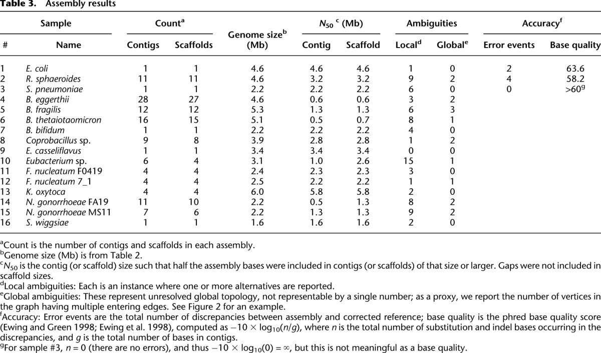
This process yields graph assemblies (Fig. 2).
Figure 2.

ALLPATHS-LG assemblies of three finished genomes. Vertices in the graph represent completely determined sequences, whereas an edge labeled n represents n possibilities for the sequence lying between its vertex sequences. For n > 1, these are local ambiguities. (1) E. coli. The assembly represents a circular chromosome that is completely determined except for a single local ambiguity for which there are two alternatives, as denoted by the edge labeled 2. This ambiguity represents either a T or a G. (2) R. sphaeroides. Each component of the graph is circular and corresponds to either a chromosome or plasmid, except for plasmids 4 and 5, which are highly similar and joined together in the assembly, resulting in two global ambiguities. The nine edges with labels exceeding 1 represent local ambiguities. (3) S. pneumoniae. The assembly is a circle. There are six local ambiguities.
The assemblies generated by this method can contain local ambiguities, i.e., loci where two or more alternatives are possible, insofar as the assembly algorithm has been able to determine. We note that such ambiguities could be due to systematic sequencing errors, or repeat copies that could not be distinguished, or actual mixed sites in the input DNA sample. For prokaryotes, these can arise as mutations in the growing culture. Of course, for eukaryotic genomes, allelic polymorphism would also give rise to local ambiguities. Assemblies can also contain global ambiguities, representing large-scale features that are not fully resolved in the assembly (Fig. 2).
The graph assemblies that we display here (Figs. 2, 3; Supplemental Fig. 3) have the following semantics. Vertices represent completely known sequences. Edges between two vertices represent the n possible sequences that could occur between the vertices and are labeled accordingly. Usually n ≥ 2, because otherwise the edge would have been absorbed into one of the vertices, but the case n = 1 can occur where there is branching in the graph (corresponding to global ambiguity), and the case n = 0 corresponds to a gap.
Figure 3.

Increased jump coverage simplifies assembly of Eubacterium. Two assemblies (A) and (B) of sample #10 (Eubacterium sp.) are shown. The assembly algorithm was applied identically in both cases; however, for B, jump coverage was increased by 2.5-fold.
To make these graph assemblies accessible to existing pipelines, we convert them into standard FASTA assembly files by selectively introducing breaks at branch points. We note that work in progress by the community will likely lead to a common format for representing the actual content of these assemblies and those produced by other groups (DB Jaffe, I MacCallum, DS Rokhsar, and MC Schatz, in prep.).
The assembly algorithm is implemented as part of ALLPATHS-LG and is automatically invoked if long-read data are provided as input to the algorithm.
Results
Data
We chose 16 bacterial samples to apply our new method to (Table 2). Reference sequences for three of these samples—Escherichia coli (Blattner et al. 1997), Streptococcus pneumoniae (Tettelin et al. 2001), and Rhodobacter sphaeroides—were available, allowing us to use them as known controls. In addition to the three control genomes, the remaining samples were selected on the basis of availability, with the exception of a single sample that was excluded after data generation because its jumping library failed. We note a wide range of GC content, from 27% to 69%, thus providing a test of performance at GC extremes.
Table 2.
Samples
For each sample, we generated data in accordance with the recipe of Table 1 (for protocols, see Supplemental Methods). In most cases, the Illumina data sets were generated by pooling 24 libraries within a single lane. Delivered coverage levels varied depending on production conditions, and we deliberately lowered coverage in some cases to get closer to the Table 1 specifications (Supplemental Tables 2–4), using an initial genome size estimate, prior to assembly. Note also that coverage levels are difficult to interpret. For example, for R. sphaeroides, we had nominal long read coverage in Pacific Biosciences data of 206×, but coverage by reads ≥2 kb was only 1.6×, whereas for E. coli, nominal read coverage was 64×, but coverage by reads ≥2 kb was 10.6× (Supplemental Table 3b). The primary contributor to this variation is likely variability in production conditions, which is unsurprising given how recently the technology was introduced.
Reference sequences
For three of our samples (#1–#3), finished reference sequences were available to compare to; however, in each case, we observed discrepancies between the reference and our sequence reads. To assess the quality of both our assemblies and the reference sequences rigorously, it was necessary to resolve all of these discrepancies. In previous work (MacCallum et al. 2009), we have described and validated reference sequence corrections for samples #1–#2: E. coli, six corrections, and R. sphaeroides, 374 corrections. We note that some of these corrections involved multiple bases, and in some cases, large-scale rearrangements of the reference sequences were corrected. In this study, we make additional corrections: one for E. coli, and 32 for R. sphaeroides.
For sample #3, S. pneumoniae, we had access not only to our data from our sample, but also to the primary sequence read data from which the finished reference was generated, enabling a comprehensive analysis of the discrepancies between the original reference sequence and our new read data, which could also account for true sequence differences between the two samples themselves. We describe here in detail the nature of the discrepancies, validation methods, and results. First, we note that discrepancies could be due to (1) errors in our data or analysis, or (2) errors in the original reference sequences, or (3) true biological differences between the sample used to create the reference sequence and our sample for this work. While we could not resolve this completely without access to the original DNA sample and extensive laboratory experiments, as we explain below, we were nonetheless able to estimate the error rate in the original reference sequence accurately.
We observed 63 discrepancies between the S. pneumoniae reference sequence and our data. An initial investigation suggested that in 60 of these cases, our sample was correctly called as different from the original reference. The other three cases were likely sites that are mixed in the population, for which either of two alternatives could be chosen as ‘correct’ (see Supplemental Table 7). We note that three of the discrepancies (including two of the mixed sites) occur within a complex 13-kb repeat region, whose exact sequence could not be determined with the available data, and that we are thus limited in our ability to draw conclusions about the accuracy of assemblies of this region. We next edited the reference to introduce these ‘corrections,’ yielding a corrected reference sequence. Next, we aligned all of our Illumina reads to both the corrected reference and the original reference, and counted those reads that supported one reference but not the other (Supplemental Table 7). These counts were overwhelmingly supportive of the corrections, with support typically in the range of 100 to 1 for the corrected reference, with the exception of the putatively mixed sites, as expected. This gave us confidence that most if not all of our ‘corrections’ were bona fide differences between our sample and the original reference sequence.
We next obtained the 26,174 original Sanger-chemistry reads for the S. pneumoniae project. We aligned these reads to the original reference, then manually investigated the discrepancies by directly examining the Sanger chemistry traces, producing a report in each case (summary in Supplemental Table 7; Supplemental Fig. 2). In summary, we found that 36 of the 63 discrepancies appeared clearly supported by the data as errors in the reference sequence, and 16 appeared to be due to bona fide differences between the two samples. The status of the remaining 11 discrepancies could not be ascertained from the available sequence read evidence.
Finally, we carried out additional laboratory work for 55 of the discrepancies to determine the exact sequence present in our sample, using PCR and Sanger sequencing as in Grad et al. (2012). In all cases, we found that the new Sanger reads support our changes.
In summary, we note that while it is impossible to know the exact number of error events in each of the reference sequences for samples #1–#3, we know that for:
E. coli, the number of error events likely is at most seven, and possibly less, since such a small number of discrepancies could be attributable to sample mutations;
S. pneumoniae, the number of error events is probably between 36 and 47;
R. sphaeroides, the number of error events is probably close to 400, because it seems very unlikely that such a large number of discrepancies could be attributable to differences in DNA sequence between the samples.
Assemblies
We next applied the assembly algorithm to all 16 data sets (ALLPATHS-LG revision 41343; computational performance shown in Supplemental Table 8), using default parameters in each case, then assessed the assemblies (Table 3). For the control assemblies #1–#3, we could use the corrected reference sequences to assay accuracy precisely.
Table 3.
Assembly results
We first describe the three control assemblies (Fig. 2; Table 3). We note that the table accounts for all imperfections in assemblies.
For E. coli, there is a single circular contig, which is completely determined except for a single base. Thus, the entry in Table 3 shows one local ambiguity. There are two errors, both substitutions, separated by three bases.
For R. sphaeroides, which has two chromosomes and five plasmids, there are 11 contigs. The extra four contigs are accounted for by the fact that two of the plasmids share an essentially perfect 19-kb repeat and are consequently glued together in the assembly, forming a ‘twinned’ plasmid structure (Fig. 2). All other chromosomes and plasmids are present as simple circles. There are nine local ambiguities, involving 2, 2, 3, 5, 6, 14, 15, 17, and 21 alternatives, respectively, representing uncertainty about the exact sequence of short regions of size up to ∼100 bases, and occurring mostly in repeat regions. Relatively large numbers of alternatives (e.g., 21) typically arise where several bases are ambiguous, resulting in an exponential growth of alternatives. There are four errors, consisting of three substitutions and one single-base deletion (G16 → G15).
For S. pneumoniae, there is a single circular contig. There are six local ambiguities. There are no errors.
Critically, we note that (1) in all three cases, there are no gaps; (2) the contigs for these projects are essentially complete chromosomes (or plasmids); and (3) the overall accuracy is substantially higher than the finished reference sequences for the same genomes. In particular, we note that there were only four incorrect bases for our assembly of R. sphaeroides, as compared with several hundred error events for the reference sequence (many involving multiple bases), and none for our assembly of S. pneumoniae, as compared with more than 30 for the reference.
We note that the overall contiguity of the 16 assemblies is very high: the median N50 contig size is 2.2 Mb (Table 3). Although we cannot assess the accuracy of the 13 ‘unknown’ genomes, we can describe their global properties (Supplemental Fig. 3). For example, three of the assemblies (#7, #9, #16) are again simple circles.
Some of the assemblies are completely resolved except for large-scale global features. For example, #10 (Eubacterium sp.) is a circle having a single global ambiguity, consisting of two parallel branches of size 0.5 Mb, flanked by 12.7-kb perfect inverted repeats that are not bridged by the data. In contrast, as suggested by the number of contigs, scaffolds, and global ambiguities, some assemblies are less well resolved. To understand why this might be the case, we computed the expected number of jumping pairs that would bridge windows of specified size (Supplemental Table 4a). For example, for 2-kb windows, among samples, this number varies from 28 to 285 (factor of 10), whereas for 6-kb windows, the number varies from 0.2 to 15 (factor of 75). These data suggest that for particular samples, the presence of somewhat longer repeats and/or somewhat less successful jumping libraries could easily result in failure to bridge all repeats, and thus a less well-resolved assembly.
To a certain extent, less successful jumping libraries can be compensated for by increasing coverage. Thus, as an experiment, we enlarged the jump data set for sample #10 by 2.5-fold by using the full amount of data that had been generated, resulting in a striking simplification of the assembly graph (Fig. 3). Indeed, because library construction rather than Illumina sequencing per se is the primary driver of assembly cost for our model, increasing coverage is in general practical. However, without going to extremes, it is limited in its effect, because intrinsic variation in jumping library ‘bridging capacity’ exceeds 10-fold between samples, and the capability of a given library to bridge repeats of a given size decreases roughly exponentially, by n-fold for each kilobase increase in the repeat size (Supplemental Table 4a), where n ranges from ∼2 to 4, depending on library quality.
Discussion
Perfection of bacterial genome assembly is an important goal since imperfections, like missing genes, misassemblies, or miscalled bases may result in incorrect biological conclusions being made regarding the biology and evolutionary history of the sequenced organism (Fraser et al. 2002; Klassen and Currie 2012). In the early days of sequencing bacterial genomes, great energy and resources were expended to finish bacterial genomes into their full circular forms, which was acceptable because the pace of sequencing itself was slow. As newer and faster methodologies and sequencing technologies arrived, perfection was increasingly sacrificed for speed and cost. Draft genome assemblies can now be rapidly produced, but they are far from perfect. In this study, we present a new recipe that relies on fast sequencing technologies and a new assembly methodology. The resulting assemblies appear at least in some cases to be better than the finished genome reference sequences produced in the past and yet can be produced rapidly at a cost that is about an order of magnitude lower (see “Supplemental Analysis”).
Our method starts with three data types, whose accuracy, evenness of coverage, and range of repeat resolution span a wide range and are compensatory, thus enabling the results presented here. We consider the natural question of whether fewer ingredients could be used. First, it is plausible that a substantially modified algorithm could omit data type A (fragment read pairs), because jumping reads might provide high-quality coverage in their place. Second, omission of data type B (long reads) cuts at the heart of the method and would be expected to have deleterious effects. We tested this: for example, for seven of the 16 samples, the N50 contig size is >10-fold smaller without these data (Supplemental Table 9). Finally, direct measurement of bridging power (Supplemental Tables 3a, 4a) indicates that even the best long reads generated here have substantially less power than jumping pairs for linking over distance; however, this could change with improvements to technology.
We note that, beyond generating longer long reads, improvements to laboratory technology could improve results. For example, amplification bias might be further reduced (Aird et al. 2011). This would have significance for medically important pathogens at GC extremes such as Mycobacterium tuberculosis (high GC) and Plasmodium falciparum (low GC). Similarly, we have seen significant variability in the ability of jumping libraries to bridge long repeats (Supplemental Table 3a). This variability may be rooted in DNA extraction protocols or the jumping library protocol itself, both of which might be improved. Moreover, we note that the methods described here are designed for DNA from culturable bacterial strains, and that their extension to amplified material from single cells could prove challenging.
We have demonstrated a computational method that is fully automated and pushbutton, using default arguments for all samples. Our method achieves exceptionally high accuracy, and we note that this is achieved by explicitly encoding ambiguities that represent uncertainty regarding the true sequence of the genome. It would be valuable to classify such ambiguities, for example, to distinguish between positions that are mixed in the sample and those that are uncertain because of limitations in the resolving power of the data. Our methods have been demonstrated only on bacterial genomes because changes to the algorithm would be needed to assemble significantly larger genomes. This would be eased by any future reductions in the error rate of the long read data. We note that at present, cost considerations might preclude generation of data by our recipe for large genomes. With changes to algorithms, coverage requirements might be reduced; however, we have not carefully controlled for coverage in this study because it would be difficult to do so meaningfully, given sample-to-sample variability.
With this work we make clear that it is now possible to rapidly generate bacterial genome assemblies that are nearly perfect, at relatively low cost. Importantly, using our approach, these high-quality genome assemblies could be generated by any researcher with access to sequence data and computational infrastructure. This capability will be critical for interpreting genomics-based studies of bacteria such as those being applied to studies of bacterial epidemiology, which require precise information to track the emergence and spread of virulence and antibacterial resistance among bacterial populations infecting humans (Harris et al. 2010; Lieberman et al. 2011; Parkhill and Wren 2011; Rasko al. 2011b; Grad et al. 2012). In general, the goal of driving genome assemblies to perfection remains important for the field.
Methods
Laboratory methods
For Illumina sequencing, 180-bp insert fragment and ∼3-kb jumping whole genome shotgun libraries were generated and sequenced with 101-base paired-end reads on an Illumina HiSeq 2000 instrument using standard methods (for more details, see Supplemental Methods). Jumping libraries were size-selected using magnetic beads rather than agarose gel, thus yielding a wide size distribution. For Pacific Biosciences sequencing, ∼3 kb (plus 6 kb and 10 kb for samples #4 and #8) insert whole genome shotgun libraries were generated and sequenced on a Pacific Biosciences RS instrument using standard methods (for more details, see Supplemental Methods).
Computational methods
The algorithm is as described above, with further details provided here and in Supplemental Methods. In particular, after converting each long read into a sequence of unipaths, we then form the ‘consensus’ of these sequences (algorithm Step II.2 above, and Supplemental Methods). In brief, starting from these sequences, we carry out a local voting process that involves choosing between two parallel branches in a bubble. This yields a collection of sequences s (each itself a sequence of unipaths). From these, we form two sets of sequences of unipaths that we call their ‘consensus.’ One consists of one-sided left and right neighborhoods of each unipath u, extending up to a fixed length (600 k-mers beyond u), and drawn from subsequences of the sequences s. The second consists of sequences constructed from s and bridging between two unipaths of size ≥1000 k-mers, but otherwise unbounded in length.
Data access
The raw data are available via NCBI GenBank (http://www.ncbi.nlm.nih.gov/genbank). Accession numbers are listed in Supplemental Tables 5 and 6. The three modified reference sequences and 16 assemblies are accessioned in GenBank by the following identifiers, which should all be suffixed with ‘01000000’): #1 (DAAD = reference; AKVX = assembly), #2 (AKVW = reference; AKBU = assembly), #3 (AKVY = reference; AKBW = assembly), #4 (AKBX), #5 (AKBY), #6 (AKBZ), #7 (AKCA), #8 (AKCB), #9 (AKCC), #10 (AKCD), #11 (AKCE), #12 (AKBT), #13 (AKCF), #14 (AKCG), #15 (AKCH), and #16 (AKCI). The full data sets of reads and assemblies are also available on the Broad Institute website at ftp://ftp.broadinstitute.org/pub/papers/assembly/Ribeiro2012.
Acknowledgments
We thank Emma Allen-Vercoe, Laurie Comstock, James Fox, Glenn R. Gibson, Jacques Izard, Janet Manson, H. Steven Seifert, Christopher Sibley, Nancy Taylor, Claudette Thompson, Marin Vulic, and Louise Williams for access to DNA samples. We thank the Broad Institute Sequencing Platform for generating the data for this work. We thank Kathryn Keho and the team at Pacific Biosciences for their support. We thank Nick Patterson for proposing the statistical model that we used to calculate separations using jumping pairs. We thank Ashlee Earl for help with sample acquisition, and helpful comments on the manuscript. We thank Andi Gnirke, Michael Ross, and Mike Zody for valuable discussions about the work. This project has been funded in part with Federal funds from the National Human Genome Research Institute, National Institutes of Health, Department of Health and Human Services, under grants R01HG003474 and U54HG003067; and in part with Federal funds from the National Institute of Allergy and Infectious Diseases, National Institutes of Health, Department of Health and Human Services, under Contract No. HHSN272200900018C.
Footnotes
[Supplemental material is available for this article.]
Article published online before print. Article, supplemental material, and publication date are at http://www.genome.org/cgi/doi/10.1101/gr.141515.112.
Freely available online through the Genome Research Open Access option.
References
- Aird D, Ross MG, Chen WS, Danielsson M, Fennell T, Russ C, Jaffe DB, Nusbaum C, Gnirke A 2011. Analyzing and minimizing PCR amplification bias in Illumina sequencing libraries. Genome Biol 12: R18 doi: 10.1186/gb-2011-12-2-r18 [DOI] [PMC free article] [PubMed] [Google Scholar]
- Bentley DR, Balasubramanian S, Swerdlow HP, Smith GP, Milton J, Brown CG, Hall KP, Evers DJ, Barnes CL, Bignell HR, et al. 2008. Accurate whole human genome sequencing using reversible terminator chemistry. Nature 456: 53–59 [DOI] [PMC free article] [PubMed] [Google Scholar]
- Blattner FR, Plunkett G III, Bloch CA, Perna NT, Burland V, Riley M, Collado-Vides J, Glasner JD, Rode CK, Mayhew GF, et al. 1997. The complete genome sequence of Escherichia coli K-12. Science 277: 1453–1462 [DOI] [PubMed] [Google Scholar]
- Butler J, MacCallum I, Kleber M, Shlyakhter IA, Belmonte MK, Lander ES, Nusbaum C, Jaffe DB 2008. ALLPATHS: De novo assembly of whole-genome shotgun microreads. Genome Res 18: 810–820 [DOI] [PMC free article] [PubMed] [Google Scholar]
- Chain PSG, Grafham DV, Fulton RS, FitzGerald MG, Hostetler J, Muzny D, Ali J, Birren B, Bruce DC, Buhay C, et al. 2009. Genome project standards in a new era of sequencing. Science 326: 236–237 [DOI] [PMC free article] [PubMed] [Google Scholar]
- Chaisson MJ, Pevzner PA 2008. Short read fragment assembly of bacterial genomes. Genome Res 18: 324–330 [DOI] [PMC free article] [PubMed] [Google Scholar]
- Chapman JA, Ho I, Sunkara S, Luo S, Schroth GP, Rokhsar DS 2011. Meraculous: De novo genome assembly with short paired-end reads. PLoS ONE 6: e23501 doi: 10.1371/journal.pone.0023501 [DOI] [PMC free article] [PubMed] [Google Scholar]
- Eid J, Fehr A, Gray J, Luong K, Lyle J, Otto G, Peluso P, Rank D, Baybayan P, Bibillo A, et al. 2009. Real-time DNA sequencing from single polymerase molecules. Science 323: 133–138 [DOI] [PubMed] [Google Scholar]
- Ewing B, Green P 1998. Base-calling of automated sequencer traces using phred. II. Error probabilities. Genome Res 8: 186–194 [PubMed] [Google Scholar]
- Ewing B, Hillier L, Wendl MC, Green P 1998. Base-calling of automated sequencer traces using phred. I. Accuracy assessment. Genome Res 8: 175–185 [DOI] [PubMed] [Google Scholar]
- Fraser CM, Eisen JA, Nelson KE, Paulsen IT, Salzberg SL 2002. The value of complete microbial sequencing (you get what you pay for). J Bacteriol 184: 6403–6405 [DOI] [PMC free article] [PubMed] [Google Scholar]
- Gnerre S, MacCallum I, Przybylski D, Ribeiro FJ, Burton JN, Walker BJ, Sharpe T, Hall G, Shea TP, Sykes S, et al. 2011. High-quality draft assemblies of mammalian genomes from massively parallel sequence data. Proc Natl Acad Sci 108: 1513–1518 [DOI] [PMC free article] [PubMed] [Google Scholar]
- Grad YH, Lipsitch M, Feldgarden M, Arachchi HM, Cerqueira GC, Fitzgerald M, Godfrey P, Haas BJ, Murphy CI, Russ C, et al. 2012. Genomic epidemiology of the Escherichia coli O104:H4 outbreaks in Europe, 2011. Proc Natl Acad Sci 109: 3065–3070 [DOI] [PMC free article] [PubMed] [Google Scholar]
- Harris SR, Feil EJ, Holden MT, Quail MA, Nickerson EK, Chantratita N, Gardete S, Tavares A, Day N, Lindsay JA, et al. 2010. Evolution of MRSA during hospital transmission and intercontinental spread. Science 327: 469–474 [DOI] [PMC free article] [PubMed] [Google Scholar]
- Klassen JL, Currie CR 2012. Gene fragmentation in bacterial draft genomes: extent, consequences and mitigation. BMC Genomics 13: 14 doi: 10.1186/1471-2164-13-14 [DOI] [PMC free article] [PubMed] [Google Scholar]
- Kyrpides NC 1999. Genomes OnLine Database (GOLD 1.0): A monitor of complete and ongoing genome projects world-wide. Bioinformatics 15: 773–774 [DOI] [PubMed] [Google Scholar]
- Li R, Fan W, Tian G, Zhu H, He L, Cai J, Huang Q, Cai Q, Li B, Bai Y, et al. 2010. The sequence and de novo assembly of the Giant Panda genome. Nature 463: 311–317 [DOI] [PMC free article] [PubMed] [Google Scholar]
- Lieberman TD, Michel JB, Aingaran M, Potter-Bynoe G, Roux D, Davis MR Jr, Skurnik D, Leiby N, LiPuma JJ, Goldberg JB, et al. 2011. Parallel bacterial evolution within multiple patients identifies candidate pathogenicity genes. Nat Genet 43: 1275–1280 [DOI] [PMC free article] [PubMed] [Google Scholar]
- MacCallum I, Przybylski D, Gnerre S, Burton J, Shlyakhter I, Gnirke A, Malek J, McKernan K, Ranade S, Shea TP, et al. 2009. ALLPATHS 2: Small genomes assembled accurately and with high continuity from short paired reads. Genome Biol 10: R103 doi: 10.1186/gb-2009-10-10-r103 [DOI] [PMC free article] [PubMed] [Google Scholar]
- Nagarajan H, Butler JE, Klimes A, Qiu Y, Zengler K, Ward J, Young ND, Methé BA, Palsson BØ, Lovley DR, et al. 2010. De novo assembly of the complete genome of an enhanced electricity-producing variant of Geobacter sulfurreducens using only short reads. PLoS ONE 5: e10922 doi: 10.1371/journal.pone.0010922 [DOI] [PMC free article] [PubMed] [Google Scholar]
- Parkhill J, Wren BW 2011. Bacterial epidemiology and biology—lessons from genome sequencing. Genome Biol 12: 230 doi: 10.1186/gb-2011-12-10-230 [DOI] [PMC free article] [PubMed] [Google Scholar]
- Pevzner PA, Tang H, Waterman MS 2001. An Eulerian path approach to DNA fragment assembly. Proc Natl Acad Sci 98: 9748–9753 [DOI] [PMC free article] [PubMed] [Google Scholar]
- Rasko DA, Webster DR, Sahl JW, Bashir A, Boisen N, Scheutz F, Paxinos EE, Sebra R, Chin CS, Iliopoulos D, et al. 2011a. Origins of the E. coli strain causing an outbreak of hemolytic-uremic syndrome in Germany. N Engl J Med 365: 709–717 [DOI] [PMC free article] [PubMed] [Google Scholar]
- Rasko DA, Worsham PL, Abshire TG, Stanley ST, Bannan JD, Wilson MR, Langham RJ, Decker RS, Jiang L, Read TD, et al. 2011b. Bacillus anthracis comparative genome analysis in support of the Amerithrax investigation. Proc Natl Acad Sci 108: 5027–5032 [DOI] [PMC free article] [PubMed] [Google Scholar]
- Simpson JT, Durbin R 2012. Efficient de novo assembly of large genomes using compressed data structures. Genome Res 22: 549–556 [DOI] [PMC free article] [PubMed] [Google Scholar]
- Simpson JT, Wong K, Jackman SD, Schein JE, Jones SJ, Birol I 2009. ABySS: A parallel assembler for short read sequence data. Genome Res 19: 1117–1123 [DOI] [PMC free article] [PubMed] [Google Scholar]
- Tettelin H, Nelson KE, Paulsen IT, Eisen JA, Read TD, Peterson S, Heidelberg J, DeBoy RT, Haft DH, Dodson RJ, et al. 2001. Complete genome sequence of a virulent isolate of Streptococcus pneumoniae. Science 293: 498–506 [DOI] [PubMed] [Google Scholar]
- Zerbino DR, Birney E 2008. Velvet: Algorithms for de novo short read assembly using de Bruijn graphs. Genome Res 18: 821–829 [DOI] [PMC free article] [PubMed] [Google Scholar]