Modeling and Dynamical Analysis of Virus-Triggered Innate Immune Signaling Pathways

Abstract

The investigation of the dynamics and regulation of virus-triggered innate immune signaling pathways at a system level will enable comprehensive analysis of the complex interactions that maintain the delicate balance between resistance to infection and viral disease. In this study, we developed a delayed mathematical model to describe the virus-induced interferon (IFN) signaling process by considering several key players in the innate immune response. Using dynamic analysis and numerical simulation, we evaluated the following predictions regarding the antiviral responses: (1) When the replication ratio of virus is less than 1, the infectious virus will be eliminated by the immune system’s defenses regardless of how the time delays are changed. (2) The IFN positive feedback regulation enhances the stability of the innate immune response and causes the immune system to present the bistability phenomenon. (3) The appropriate duration of viral replication and IFN feedback processes stabilizes the innate immune response. The predictions from the model were confirmed by monitoring the virus titer and IFN expression in infected cells. The results suggest that the balance between viral replication and IFN-induced feedback regulation coordinates the dynamical behavior of virus-triggered signaling and antiviral responses. This work will help clarify the mechanisms of the virus-induced innate immune response at a system level and provide instruction for further biological experiments.

Introduction

In recent years, there has been an explosion of interest in the innate immune response [1]–[5] because it is now known that most infectious pathogens are eliminated through the innate immune response without necessarily requiring the activation of adaptive immunity [6]–[8]. The application of systems biology tools to the innate immune system will enable comprehensive analysis of the complex interactions that maintain the balance between resistance to infection and disease [9], [10].

Mathematical modeling and theoretical analyses are increasingly being used to investigate the control mechanism and to identify the coordination of interferon (IFN)-induced JAK-STAT signaling pathways [11]–[15]. The integration of experimental studies with mathematical models of virus-triggered signaling pathways during the primary response was used to explore the effects of viral proteins on type I IFN induction [16], but the late phase of viral infection was not considered. In fact, there are two main phases in type I IFN expression and regulation induced by viral infection [17], [18] (Figure 1). In the early phase of viral infection, IFN-regulatory factor 3 (IRF3) and IRF7 are phosphorylated at specific serine residues, resulting in the homodimerization or heterodimerization of the IRF3 and IRF7. These dimers then translocate to the nucleus and induce the expression of chemokines and small amounts of IFNβ (and IFNα). In the late phase of infection, progeny viruses are produced and released from infected cells. Simultaneously, newly synthesized IFNs bind to the type I IFN receptor (IFNAR) and activate the expression of numerous IFN-stimulated genes (ISGs) via the JAK/STAT pathway. The IFNs then induce the transcription of the IRF7 gene, leading to increases in the expression of the IFNβ and IFNα proteins and, thus, promoting the production of many antiviral proteins (such as Mx, ISG20, OAS and PKR) and immunoactive cytokines. These antiviral components inhibit viral replication and cause apoptosis of infected cells, subsequently resulting in the clearance of the infectious pathogens.

Figure 1. A Schematic reaction diagram of virus-triggered IFN pathways.

There are two main phases in type I IFN (IFNα/β) gene expression and regulation by viral infection. In phase I of an infection with viruses, a small amount of IFNβ is induced by the virus. Then, the expressed IFNβ activates the JAK-STAT pathway in phase II, inducing the generation of a large number of IFNα/β and AVPs which inhibits viral replication.

To the best of our knowledge, the modeling of the complex process of virus-mediated innate immune response has not been reported in the literature. To better understand the dynamics of the innate immune response and the regulation of the signaling components, we develop a simplified model of virus-activated signaling pathways in the innate immune response. In our model, the interactions between the following components are considered, that is, viral mRNA produced from viral infection (viral mRNAs), type I interferon (IFNs) and antiviral proteins (AVPs) (Figure 2). Dynamical theory and numerical simulations are used to analyze the dynamical features of the virus-triggered innate immune response. Some predictions based on the model are validated by biological experiments.

Figure 2. A simplified reaction scheme considered in the mathematical model.

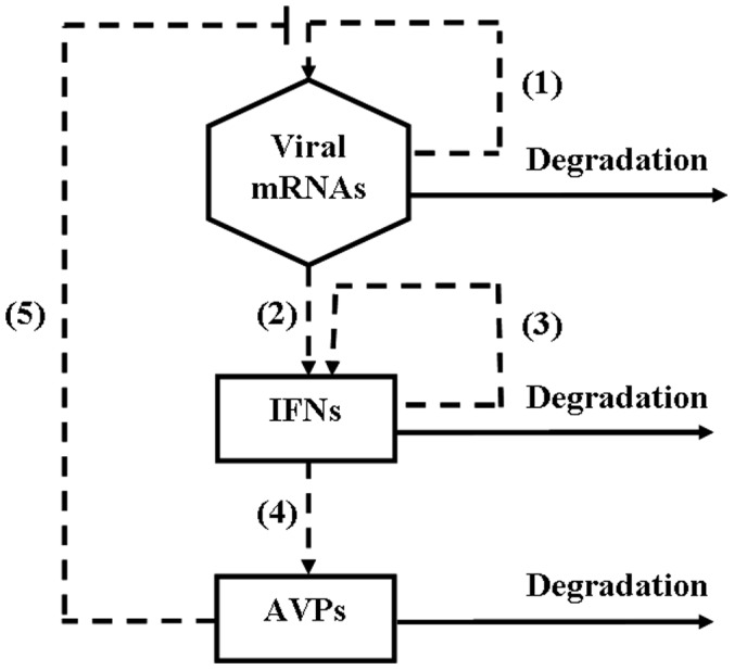
There are three main components (viral mRNAs, IFNs and AVPs) and five reactions: (1) the replication of viral mRNAs; (2) the virus-activated IFN expression; (3) the positive feedback of IFNs; (4) the activation of AVPs by IFNs; (5) the inhibition of the virus by AVPs. The dashed lines indicate that there are time delays in the reactions.

Materials and Methods

Experiments

Cell culture, virus infection, and titration

Wild type VISA^+/+ and knockout VISA^−/− MEF cells (Dr. HB Shu, College of Life Sciences, Wuhan University) were used to investigate the dynamics of virus-induced IFN production and the antiviral activity of type I IFNs. The cells were propagated and maintained at 37°C with 5% CO₂ in Dulbecco’s Modified Eagle Medium (DMEM) (Invitrogen, Carlsbad, CA, USA) supplemented with 10% fetal bovine serum (FBS) (HyClone, Logan, Utah, USA), penicillin (100 units/ml) and streptomycin (100 µg/ml). Vesicular stomatitis virus-expressing fluorescent reporter GFP (VSV*GFP) was used to measure viral replication and IFNβ activity. For viral infection, the cells (5×10⁵ per well) were seeded in 6-well plates and incubated overnight. VSV*GFP was added to each well at 0.05 MOI in 500 µl and incubated for 1 h at 37°C. The wells were washed once with phosphate-buffered saline (PBS) and then 1 ml of growth medium was added. The viral stock was collected at the indicated times postinfection (p.i.). For virus titration, a tissue culture infectious dose 50 (TCID₅₀) based on the end-point dilution of the virus at which a cytopathic effect (CPE) is detected in 50% of the cell culture replicates infected by a given amount of virus is employed. The CPE induced by VSV*GFP was observable under a fluorescence microscope at 1–2 days p.i. The VSV*GFP titer was determined using 96-well plates in duplicate from the TCID₅₀ of 10-fold serial dilutions (1∶10¹ to 1∶10⁷) of Opti-MEM (Invitrogen) and was expressed as PFU/ml by calculating the TCID₅₀. A fluorescence-activated cell sorting (FACS) assay was further used to quantify VSV*GFP titer in infected cells [19]. In brief, wt VISA^+/+ and VISA^−/− cells were plated in flat-bottom 6-well plates in DMEM at 5×10⁵ cells each well and incubated at 37°C and 5% CO₂ overnight. 0.05 MOI of VSV*GFP in 500 µl was added to well. After incubation for the indicated times, the cells were washed with cold PBS and incubated with 100 µl of 0.25% Trypsin-EDTA (Gibco, Carlsbad, CA) at 37°C for 5 minutes. The Cells were pelleted by centrifugation at 1600 rpm and washed twice in PBS with 0.1% saponin. Next, the cells were re-suspended in FACS buffer (PBS, 1% FCS and 0.5% sodium azide), and analyzed on the FACSCalibur Flow Cytometer (BD Biosciences, Franklin Lakes, NJ). Virus-positive populations were determined by negatively gating on uninfected samples.

VSV-based IFN bioassay

The IFN concentration was measured by a bioassay based on the IFNα/β-mediated VSV growth reduction as previously described [20], [21]. Wt VISA^+/+ and VISA^−/− cells were infected with Sendai virus and at the indicated times, supernatants were collected for measurement of IFNβ concentration. Approximately 1×10⁴ cells were seeded into each well of a 96-well plate and incubated overnight at 5% CO₂ and 37°C. The cells were then treated either with serial dilutions of standard IFN or serial 10-fold dilutions of IFN-containing samples in 100 µl of growth medium for the indicated times. Subsequently, the growth medium was removed and 1×0.01 MOI of VSV*GFP in 100 µl of infection medium (DMEM with 2% FCS) was added to each well. After 24–48 hrs of further incubation, the cells were observed under a fluorescence microscope and the viral titer was expressed as PFU/ml by counting the TCID₅₀.

Models

Mathematical model and nondimensionalization

In this study, the two phases of viral infection were considered. The graphical representation of the mathematical model including the three components and reactions considered is depicted in Figure 2. Upon viral infection, we considered five reactions: (1) the replication of viral mRNAs, (2) the virus-activated IFN expression, (3) the positive feedback of IFNs, (4) the expression of AVPs activated by IFNs and (5) the inhibition of virus replication by AVPs. Because these reactions include the multistep reaction processes which need to take the time to finish, we introduced time delays to describe them for the simplicity. The concentration of reactant that changes over time can be described by an ordinary differential equation (ODE).

where and represent the production rate and the degradation rate of reactant , respectively. Based on the law of mass action, we assume that the production rates for three reactions ((1), (2) and (4)) and the degradation rates of three components are linearly proportional to their concentrations. The rates for reactions (3) and (5) are represented using Hill functions. In this paradigm, the dynamics of this network is determined by a system of nonlinear ordinary differential equations (ODEs).

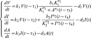(1)

where V (mol/L), I (mol/L) and A (mol/L) are the concentrations of viral mRNAs, IFNs and AVPs, respectively.

In model (1), there are five time delays. Two time delays and are related to the two processes (1) and (5) that require an intrinsic discrete time to be accomplished. The other three time delays (, and ) are associated with the three reactions ((2), (3) and (4)) that include the multistep reaction processes not described in detail in the model. The definitions of all parameters in model (1) are described at the first and second columns of Table 1.

Table 1. The definitions and values of all parameters in model (1).

Parameters	Process or Description	Range	Reference	Value	Unit
k 1	The kinetic rate constant of the viral replication	–	Estimated	4	h−1
k 2	The activation rate constant of IFNs induced by viruses	–	Estimated	0.3	h−1
k 3	The activation rate constant of AVPs induced by IFNs	–	Estimated	0.1	h−1
d 1	The degradation rate of viral mRNAs	0.1	[22]	0.1	h−1
d 2	The degradation rate of IFNs	0.1∼0.7	[23]	0.7	h−1
d 3	The degradation rate of AVPs	0.03∼0.35	[24], [25]	0.12	h−1
b 1	The maximal production rate of the Hill function of AVPs on the viruses	–	Estimated	10	–
b 2	The maximal production rate of the Hill function of IFN positive feedback	–	Estimated	80	mol/(Lh)
K 1	The inhibition coefficient of the Hill function of AVPs on the viruses	–	Estimated	33	mol/L
K 2	The activation coefficient of the Hill function of IFN positive feedback	–	Estimated	0.1	mol/L
τ 1	The duration of the viral replication	8∼12	[22]	12	h
τ 2	The time required for virus-inducible IFN production and secretion	4∼8	[26]	8	h
τ 3	the time required for IFN-induced AVP production	2∼6	[27]–[29]	7	h
τ 4	the duration of IFN positive feedback	–	Estimated	9	h
τ 5	the delay in AVP-mediated inhibition of virus production	–	Estimated	5	h
n 1	Hill coefficient	–	Estimated	1	–
n 2	Hill coefficient	–	Estimated	1	–

Note: The degradation rate of virus, IFN or AVP amounts to ln2/T_half-life [30] and its unit is h⁻¹. The half-life of virus is about 7 hour [22], the half-life of IFN is about 1∼7 hour [23], which the half-life of IFNβ is about 1∼3 hour and the half-life of IFNα is about 4∼7 hour, and the half-life of AVP is 2∼24 hour [24], [25], which is in fact the range of the half-life of Mx protein which is a kind of important anti-virus protein.

To make the theoretical analysis convenient, we nondimensionalize the model (1). Time is scaled relative to the rate of degradation of the AVPs (d ₃). We make the following substitutions and assume that all of the model parameters are greater than 0 for the actual biological significance.

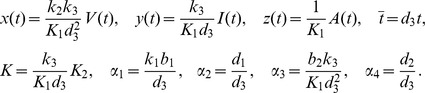Using instead of for notational convenience, we obtain the non-dimensional system of equations:

(2)

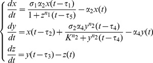
where and represent the dimensionless concentrations of viral mRNAs, IFNs and AVPs, respectively. Model (2) is determined by five dimensionless parameters α _i (i = 1,2,3,4) and K. α ₂ and α ₄ correspond to the degradation rates of the virus and IFNs divided by the rate of the degradation of AVPs (time scale), respectively, which are called their relative degradation ratios. α ₁ corresponds to the replication rate of the virus divided by the rate of the degradation of the AVPs; α ₃ corresponds to the activation rates of IFN positive feedback and the activation ratio of AVPs divided by the rate of the degradation of AVPs. K is relative to the production ratio of AVPs.

Let , and . Then we can view σ ₁, σ₂ and σ ₃ as the replication ratio of the virus, the production ratio of IFN and the relative strength of IFN positive feedback, respectively.

Numerical simulation

All numerical simulations are implemented using MATLAB 2009b (The MathWorks, Natick, MA). The system of ordinary differential equations with no delay and delay-differential equations were numerically solved by the subroutine ode45 and dde23 respectively.

Steady-state analysis and bifurcation analysis of the model

From a biological point of view, if a system possesses a stable steady state, then this corresponds to a normal biological process. In contrast, the existence of unstable steady states or oscillations corresponds to pathology, i.e., an abnormal biological process. To control the viral infection, we seek conditions on the parameters of the signaling process that can guarantee the existence of the steady states.

The steady state concentrations are obtained by solving the system of algebraic equations (2).

When n ₁ = n ₂ = 1 in system (2), there are three nonnegative steady states: a trivial steady state (O₁), which represents the absence of all components; a virus-clearance steady state (O₂), which corresponds to the host eliminating the virus and returning to its normal immune state; and a virus-latent steady state (O₃), which implies that the virus is coexisting with the host.

When n ₁ = n ₂ = 2 in system (2), there are four nonnegative steady states: a trivial steady state (), which represents the absence of all components; two virus-clearance steady states (and ), which correspond to the host eliminating the virus and returning to the normal immune state; and a virus-latent steady state (), which implies that the virus is coexisting with the host.

and

We primarily use the basic stability principle in a dynamic system [31] and the Routh-Hurwitz criterion [32] (see Supporting Information) to analyze the stability of the steady state conditions. We use the Hopf bifurcation theorem [33] to analyze the Hopf bifurcation of the system (2).

Results

Comparison between the Simulation and Experimental Viral Replication Results

VISA^+/+ MEF cells were infected with VSV*GFP and the culture supernatants were collected after 8, 12, 16, 24 and 36 hrs of incubation, respectively. Experimental data showed that virus concentration in the culture supernatants first increased and then decreased at the indicated times ant reached to a peak at 24 hrs p.i. (Figure 3(A)). Based on the real biological meanings of the three components and reaction rates, we determined the best group of parameters in the model. The parameter values of the model and the initial values used for the simulation are listed in the fifth column in Table 1 and Table 2, respectively. Figure 3 shows the consistency between the numerical simulation and the experimental results, indicating that the model is reasonable and can reflect known biological phenomena.

Figure 3. Comparison between the numerical simulation and the experimental results.

(A). The time courses of the normalized virus titers from experiments and simulation; (B). The numerical simulation of three components. The initial value is [1000, 10, 2] (Unit: mol/L) and the other parameters of the simulation are listed in Table 1.

Table 2. Initial concentration values of three components for the simulation in Figure 3.

Component	Initial Value	Unit
V(0)	100	mol/L
I(0)	10	mol/L
A(0)	2	mol/L

Antiviral Immune Responses when there is no Synergistic Effect in the IFN Positive Feedback

When all reactions are prompt and there is no synergistic effect in the IFN positive feedback, we assume that all time delays are equal to zero and the Hill coefficients n ₁ and n ₂ are equal to 1. To guarantee the existence of a stable virus-clearance steady state and a stable steady state of virus-latent infection, we performed the stability analysis on the model (see Theorem S1 in the Text S1 for details and the numerical simulation in Figure S1). For convenience to understand, the conditions on the parameters are listed in Table 3. The stability domains can also be represented graphically by three regions that are divided by three straight lines σ ₁ = 1, σ ₃ = 1, and in the σ ₁–σ ₃ plane (Figure 4).

Table 3. The stability conditions at the steady states for Hill coefficients n ₁ = n ₂ = 1.

steady-state	Stability conditions	corresponding region in Fig. 4	additional conditions
			––––
			––––

Remark: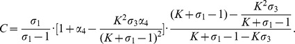

Figure 4. Schematic diagram of stability conditions without a synergistic effect.

The first quadrant in the plane σ ₁–σ ₃ is divided into three regions , and by the lines σ ₁ = 1, σ ₃ = 1, and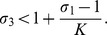

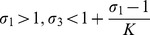
From Table 3 and Figure 4, it can be observed that either the conditions σ ₁<1 and σ ₃>1 or the conditions σ ₁>1 and 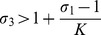guarantee the existence of a stable virus-clearance state. This result shows that the virus can be steadily eliminated by immune defenses if the relative strength of the IFNs exceeds a certain threshold value. Thus, viral infection can be eradicated from the host as long as the production of the IFNs is sufficient. If the relative strength of the IFNs is below this threshold (that is, 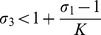), the system can exhibit two cases. One case is a trivial steady state if σ ₁<1, indicating the absence of all components. In the other case, the system exhibits a stable virus-latent state if σ ₁>1 and the relative degradation ratio of virus α ₂ does not exceed a certain threshold value (C) (A special case is presented in Corollary S1 in Text S1. In this case, the relative degradation rate of virus that is, the rate of viral degradation is less than that of AVPs). This result indicates that the infectious viruses are steadily coexisting with the host when the viral reproduction and the activation of IFNs are under controlled states. Otherwise, when the degradation rate of viral mRNAs is large (especially, the degradation of viral mRNAs is faster than that of IFNs), the system will become unstable (undergo oscillation) (see Figure 5 for the bifurcation graph and Theorem S2 for the proof in Text S1).

Figure 5. Bifurcation graph about parameter α₂ without a synergistic effect.

The dimensionless parameter α₂ is associated with the relative ratio of the viral degradation. When α ₂ = 10.2347 (), a Hopf bifurcation occurs. The fixed dimensionless parameter values are n ₁ = n ₂ = 1, σ ₁ = 4, σ ₂ = 3, α ₄ = 4 and K = 2.

Antiviral Immune Responses when there is a Synergistic Effect in the IFN Positive Feedback

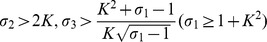
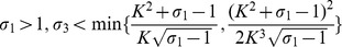
When there is a synergistic effect in the IFN positive feedback, the Hill coefficients n ₁ and n ₂ are set to be greater than one. Table 4 lists the stability conditions for three steady states and Figure 6 depicts the stability domains (see Theorem S3 and its proof in Text S1 and the numerical simulation in Figure S2).

Table 4. The stability conditions at the steady states for Hill coefficients n ₁ = n ₂ = 2.

steady-states	stability conditions	corresponding region in Fig. 6	additional conditions
			––––
			––––
	––––	––––	––––

Remark: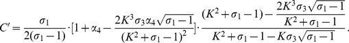

Figure 6. Schematic diagram of stability conditions with a synergistic effect.

The first quadrant in the plane σ _1– σ ₃ is divided into six regions , , , , and by the lines σ ₁ = 1, σ ₃ = 2, and the curves and

As observed in Table 4 and Figure 6, the system can reach two stable steady states, including the trivial steady state and the virus-clearance steady state, if the replication ratio of the virus σ ₁<1 and the relative strength of the IFN positive feedback σ ₃>2 (domain in Figure 6 and Figure 7(A)). We easily infer that the system is also bistable between the virus-clearance steady state and the virus-latent steady state (domain in Figure 6 and Figure 7(A)) when the conditions and σ₃>2 are satisfied, i.e., the system can either be in a virus-clearance state or in the virus-latent state depending on its history (or initial conditions). Conditions σ ₁>1 and guarantee the maintenance of a stable virus-clearance state. These results indicate that the IFN positive feedback makes the system exhibit more complicated phenomenon.

Figure 7. Bistability and bifurcation phenomena.

(A). Bistability occurs when the value of σ ₁ changes from 0 to 10, which successively pass through domains , , and (σ ₂ = 4.1) in Figure 6. (B). Bifurcation occurs when the value of σ ₁ changes from 0 to 6, which successively pass through domains , , and (σ ₂ = 3.9) in Figure 6. The other parameters are fixed: α ₂ = 0.5, α ₄ = 4, K = 2 and n ₁ = n ₂ = 2.

Figure 7(A) shows that the system (2) becomes bistable at O ₁′ or O ₂′ when σ ₁ ranges from 0 to 1 and then at O ₂′ or O ₃′ when σ ₁ ranges from 1 to 1.3253. The system (2) becomes monostable at O ₂′ when σ ₁ ranges from 1.3253 to 7.25 or at O ₃′ when σ ₁>7.25. Figure 7(B) shows that a Hopf bifurcation occurs when the value of σ ₁ changes from 0 to 6, which will successively pass through domains , , and in Figure 6 in turn. The bifurcation graph of α₂ and the simulation results under different parameter settings are depicted in Figure S3 and Figure S4, respectively. Therefore, the system (2) exhibits characteristics of switches from bistability, to monostability to oscillation and then back to monostability.

Experimental Verification of the Dynamic Characterization of Virus Replication in Infected Cells

Silencing VISA significantly decreased IFNβ production and increased virus titers in infected cells [34], [35]. Therefore, wt VISA^+/+ and VISA^−/−MEF cells were used to evaluate the effect of IFNβ on the viral replication. At the indicated times p.i.with VSV*GFP, virus titers were determined. From 0 to 8 hrs p.i., low virus titers were observed in both VISA^+/+ and VISA^−/− cells. Subsequently, virus titers increased and reached a peak at 24 hrs p.i. in both VISA^+/+ and VISA^−/− cells. Compared with VISA^+/+ cells, significantly increased virus titers were observed at 16 and 24 hrs p.i. in VISA^−/− cells (Figure 8(A)). Similarly, data of a FACS-based assay showed that a virus titer reached a peak at 24 hrs p.i. in both VISA^+/+ and VISA^−/− cells and that compared with VISA^+/+ cells, a higher virus titer at 12 and 24 hrs p.i. in VISA^−/− cells (Figure 8(B)). A FACS-based assay was believed to be an objective and reproducible method for quantification of virus titers [19], [36]. After induction with Sendai virus, a IFNβ production could be measured at 8 hrs p.i. and exhibited subsequently increased concentration at 12 and 24 hrs p.i. in VISA^+/+ cells. However, the negligible IFNβ was expressed in VISA^−/− cells from 8 to 24 hrs p.i. (Figure S5). When VISA^+/+ cells were treated with culture supernatant (IFNβ) for 6, 12, and 24 hrs, inhibtion of virus infection significantly increased with the extended treatment time. In contrast, this phenomena was not observed in VISA^−/− cells (Figure 9). These results suggest that IFNβ-mediated inhibition of viral replication is dose-dependent and that the inhibition of virus replication is enhanced by IFNβ positive feedback expression.

Figure 8. The effect of IFNβ on virus replication.

(A). Virus titers in IFNβ-producing (VISA^+/+) and IFNβ-non-producing (VISA^−/−) cells were determined by the plaque assay at the indicated times. The data represent the mean ± SD of 3 independent tests. (B). Virus titers were detected using a FACS assay. IFNβ-producing (VISA^+/+) and IFNβ-non-producing (VISA^−/−) cells were infected with 0.05 MOI of VSV*GFP and virus-infected populations were determined by negatively gating on uninfected samples at the indicated times. The virus-infected to total cells ratio (% virus positive cells) of VISA^+/+ or VISA^−/− cells are shown. The data represent the mean ± SD of 3 independent tests.

Figure 9. The kinetics of IFNβ-mediated inhibition of virus infection.

After 1×10⁴ IFNβ-producing (VISA^+/+) cells in each well (96-well plates) were treated with the supernatant containing IFNβ for the indicated times, the cells were infected with 0.01 MOI of VSV*GFP. After 24 hrs of incubation, the virus-infected wells were calculated under a fluorescence microscope. The control represents the number of virus-infected wells at the control condition (untreated with the supernatant containing IFNβ).

Consideration of the Time Delays Under Normal Response Conditions

In the simplified IFN-related pathway, we equivalently used the time delays to represent the multistep reaction processes. The impact of time delays on the system was further investigated. For convenience in the theoretical analysis, we assume that the Hill coefficients n ₁ = n ₂ = 1. We theoretically prove that the time delays have no influence on the stability of the system in the first and second steady states (see Theorem S4 and Theorem S5 for the proofs in Text S1). These theoretical results show that when the replication ratio of the virus (σ ₁) is smaller than one, the virus can be eliminated by the immune defense regardless of how the time delays are changed, indicating that the speed (fast or slow) of the chemical reaction processes has no influence on the clearance of virus. Furthermore, we simulate the case in which the Hill coefficients n ₁ and n ₂ are greater than one and also find that the time delays have no effects on the stability in the first and second steady states (Figure 10).

Figure 10. The influence of time delays on the stability of the system.

The settings of the dimensionless parameters are n ₁ = n ₂ = 2, σ ₁ = 0.5, α ₂ = 5, α ₄ = 4, K = 2, and the initial value is [10 5 2] for all. σ ₂ = 1 for A and B. σ ₂ = 5 for C and D. τ ₁ = 5, τ ₂ = 3, τ ₃ = 2, τ ₄ = 4, τ ₅ = 6 for A and C, and τ ₁ = 50, τ ₂ = 30, τ ₃ = 20, τ ₄ = 40, τ ₅ = 60 for B and D.

We further determine the influence of the time delays on the third, virus-latent steady state and find that the delays in different reaction processes have different influences on the system.

The Influence of Viral Replication and IFN Positive Feedback on the Dynamics of the System

All time delays can make the system oscillate in the third, virus-latent steady state and induce Hopf bifurcation (see Theorem S6 for the proof in Text S1). However, the effect of the duration of viral replication τ ₁ and the time for IFN positive feedback τ ₄ on the system is notable. Figure 11 illustrates the process, which moves from an oscillation system when there are no time delays (Figure 11(A)) to a steady state when there is a small delay τ ₁ (Figure 11(B)) and then back to an oscillation system when there is a large delay τ ₁ (Figure 11(C)). An appropriate range of the time of viral replication and the IFN feedback makes the system stable. The bifurcation graph about τ ₁ and τ ₄ is given in Figure 12, indicating that the system is stable and infection can be control when the duration for virus replication and IFN positive feedback is within certain range, or the system is unstable (oscillation) and infection would be sustained. From the bifurcation graph, we can also estimate that the time ranges of virus replication and the IFN feedback in innate immune system are approximately 2–10 hrs and 9–25 hrs (dimensionless time range multiply the rate of degradation of the AVPs), respectively.

Figure 11. Stabilized process of the oscillation system with time delay τ₁.

(A). τ ₁ = 0, oscillation system. (B). τ ₁ = 1, steady state. (C). τ ₁ = 3, oscillation system. Parameters: n ₁ = n ₂ = 1, σ ₁ = 4, σ ₂ = 3, α ₂ = 12 (>C = 10.2347), α ₄ = 4, K = 2. All other time delays are 0.

Figure 12. Bifurcation diagram about time delays τ₁ and τ₄.

(A). System (2) undergoes a process from oscillation to stability and then to the oscillation again when τ ₁ changes from 0 to 2. (B). System (2) undergoes a process from oscillation to stability and then to oscillation again when τ ₄ changes from 0 to 4. The dimensionless parameters are n ₁ = n ₂ = 1, σ ₁ = 4, σ ₂ = 3, α ₂ = 12 (>C = 10.2347), α ₄ = 4 and K = 2. All other time delays are 0.

Moreover, τ ₁ and τ ₄ can eliminate the oscillation caused by other three time delays τ ₂, τ ₃ andτ ₅ in three reactions ((2), (3) and (4)) in Figure 2 (Figure 13). Figure 13 indicates that the system is capable of changing from a steady state with no delays (Figure 13(A)) to oscillation with delays τ ₂, τ ₃ and τ ₅ (Figure 13(B)) and then to a steady state with a small delay τ ₁ (Figure 13(C)) and finally back again to oscillation with a large delay τ ₁ (Figure 13(D)). The time of the IFN feedback regulation τ ₄ has similar results as τ ₁ (Figure 13 (E) and (F)). When n ₁ and n ₂ are greater than 1, a large delay τ ₁ or τ ₄ can also make the system stable (Figure 14). These results demonstrated that an adaptable time delay for viral replication and IFN feedback regulation will control the dynamics of the system even if the delays of the other reaction processes affect the innate immune system, further suggesting the importance of two processes for viral replication and IFN feedback regulation.

Figure 13. From oscillation caused by the time delays to stability from the time delay τ₁.

(A). System (2) is stable when τ ₁ = τ ₂ = τ ₃ = τ ₄ = τ ₅ = 0. (B). System (2) is oscillating, induced by τ ₂, τ ₃ or τ ₅ when τ ₁ = 0, τ ₂ = 0.3, τ ₃ = 0.2, τ ₄ = 0 and τ ₅ = 0.6. (C). System (2) is stable when τ ₁ = 1, τ ₂ = 0.3, τ ₃ = 0.2, τ ₄ = 0 and τ ₅ = 0.6. (D). System (2) is oscillating when τ ₁ = 5, τ ₂ = 0.3, τ ₃ = 0.2, τ ₄ = 0 and τ ₅ = 0.6. (E). System (2) is stable when τ ₁ = 0, τ ₂ = 0.3, τ ₃ = 0.2, τ ₄ = 4 and τ ₅ = 0.6. (F). System (2) is oscillating when τ ₁ = 0, τ ₂ = 0.3, τ ₃ = 0.2, τ ₄ = 9 and τ ₅ = 0.6. Other parameters: n ₁ = n ₂ = 1, σ ₁ = 4, σ ₂ = 3, α ₂ = 2.5 (<), α ₄ = 4 and K = 2. The initial values are [10,5,2].

Figure 14. Stabilization of oscillation when Hill coefficients n₁ and n₂ are greater than one.

(A). No delays, oscillation system. (B). τ ₁ = 1, steady state. (C). τ ₄ = 5, steady state. Other dimensionless parameters: n ₁ = 4, n ₂ = 3, σ ₁ = 4, σ ₂ = 0.3, α ₂ = 2, α ₄ = 4 and K = 2. The initial values are (10, 5, 2).

Discussion

Understanding the dynamic regulation of antiviral immune responses is essential for predicting the manifestation and outcome of infectious disease. Unfortunately, as it relates to complex biological processes, the acquisition of the empirical data is usually time-consuming and intricate and is tremendously limited by both temporal and financial constraints. In recent years, computational modeling and analysis based on experimental measurements have become very important tools for predicting the intrinsic mechanisms of signaling pathways at the network level [37]. However, data-driven models of signaling networks are often complicated because there are many constant and adjustable parameters in the models, which include rate and equilibrium constants together with initial species concentrations [38], [39]. A relatively realistic method to address the problem is to identify and model only the essential feature(s) of each process in the networks [37].

The present model only considers the three important components in virus-triggered IFN signaling pathways. Thus, it is beneficial to analyze the model using dynamic theory. We theoretically obtained the quantitative relationship between the parameters in the model and analyzed the effects of model parameters and feedback mechanisms on the behaviors of the system after virus infection. Therefore, it is quite different from the models in the previous studies. In previously described models, only specific parameter sets are numerically simulated and it is not convenient to determine the influence of varying values of these parameters. The mathematical model we developed in this study will enable investigators to gain a better understanding of the virus-triggered innate immune signaling network.

To verify our theoretical results, IFNβ-producing (VISA^+/+) and IFNβ-non-producing (VISA^−/−) cells were used to investigate the dynamics of virus-induced IFN production and its antiviral response. The virus titers were directly calculated by measuring cells infected with a VSV*GFP using fluorescence microscopy and a flow cytometer. The virus titers in cells were tested at 0, 8, 12, 24, 36, 48 and 72 hrs p.i., respectively. Our results showed that the virus titer reached a peak at 24 hrs p.i. and subsequently decreased. Compared with VISA^+/+ cells, 9-fold higher peak viral titers were produced in VISA^−/− cells. Because a FACS-based assay is used to detect infected cells (not for mature virus), a higher virus titer was obtained than TCID₅₀ at 12 hrs p.i. After treatment with the culture supernatants containing IFNβ for 6, 12 and 24 hrs, respectively, cells were infected with VSV*GFP, and inhibition of the virus infection was enhanced following a prolonged treatment in VISA^+/+ cells, but not in VISA^−/− cells, suggesting that inhibition of virus replication by IFNβ was a dose-dependent manner. However, the real innate immune response processes of a host are complicated; therefore, in addition to integrating experimental studies with mathematical models, a suitable animal model will be developed to better understand the mechanisms of virus-triggered immune responses and viral diseases.

Previous studies indicated that the time delay is a key factor in the behavior of the model and that the steady state of the system is destabilized if the time delay is long enough [40–44]. In many literatures related to biological systems, a single time delay was considered because multiple time delays make the model complex and the resulting theoretical analysis difficult [45]. In this study, we consider five time delays in reaction processes. By combining the theoretical proofs with numerical simulations, we find that appropriate time delays could stabilize the system and switch it from an unstable or oscillating condition to a steady state. It appears as if time delays in innate immune responses could be beneficial in lessening the pathological damage induced by virus infection. This interesting phenomenon has not been previously described in the literature. This helps us understand more properties and regimes of the antiviral innate immune responses. So far, it is difficult to verify the effect of time delay on innate immune responses using biological experiments. The role of time delays in the system based on this model requires further exploration.

In addition, if the specific biological background used in this model is neglected, the present model can be viewed as a coupled system consisting of negative and positive feedback. Importantly, the system can switch between monostability, bistability and oscillation. The specific features of the system could be used to design a reasonable biological network and specify the corresponding biological functions.

Conclusion

In this study, we propose a simplified mathematical model with time delays for understanding the virus-triggered innate immune network. We deduce that the system can switch between monostability, bistability and oscillation with different conditions. By combining the theoretical analysis with experiment study, we find that the replication ratio of the virus is an important parameter for resulting in viral infection, virus-clearance and steady-state maintenance. If the replication ratio of the virus is less than one, then the virus is eliminated by the immune defense; and if the replication ratio of the virus is relatively high, then the stability of the system is disturbed. In this case, the system either eliminates the virus via IFN positive feedback and AVP production or causes an infectious disease. Moreover, the influence of time delays on the stability of the system depends on various steady-states. The duration of two processes for viral replication and IFN feedback can guarantee the normal innate immune response, beyond this range, the immune balance possibly is disturbed. The predictions in this study can be generalized to other viral infections. Our work indicates that modeling and dynamical analysis of virus-triggered innate immune responses have the potential to prevent excessive experimentation and to provide researchers with complementary and valuable insight into the mechanisms of signaling networks.

Supporting Information

Figure S1

Simulation of steady states and bifurcation for the system (2) without a synergistic effect. (A): System (2) at O ₁(0, 0, 0) is stable. The parameters are σ ₁ = 0.5, σ ₂ = 1, α ₂ = 5, α ₄ = 4 and K = 2, which occur in region of Figure 4. (B): System (2) at O ₂ (0, 1, 1) is stable. The parameters are σ ₁ = 0.5, σ ₂ = 3, α ₂ = 5, α ₄ = 4 and K = 2, which occur in region of Figure 4. (C): System (2) at O ₃ (4.8, 3, 3) is stable. The parameters are σ ₁ = 4, σ ₂ = 3, α ₂ = 5 (C = 10.2347), α ₄ = 4 and K = 2, which occur in region of Figure 4. (D) and (E): Hopf bifurcation phenomenon. At the same time, the system (2) at O ₁ (0, 0, 0), O ₂ (0, 1, 1) or O ₃ (4.8, 3, 3) is unstable when α ₂ = 10.2347 for (D) and α ₂ = 12 for (E). The other parameters are same: σ ₁ = 4, σ ₂ = 3, α ₄ = 4 and K = 2, which occur in region of Figure 4 but α ₂> = C does not satisfy the additional conditions. Thus a Hopf bifurcation occurs and a periodic oscillation appears. The amplitude of the periodic oscillation is greater if α ₂ is larger. The initial values are [10], [5], [2] and n ₁ = n ₂ = 1 for all simulations.

(TIF)

Figure S2

Simulation of steady states and bifurcation for the system (2) with a synergistic effect. (A) and (B): The origin is stable. (A): The parameters of σ ₁ and σ ₂ are in region of Figure 4 (σ ₂ = 1, n ₁ = n ₂ = 1, cf. Figure S1: A). B: The parameters of σ ₁ and σ ₂ are in region of Figure 4, i.e., region of Figure 6 (σ ₂ = 3, n ₁ = n ₂ = 2). The other parameters are fixed σ ₁ = 0.5, α ₂ = 5, α ₄ = 4 and K = 2. (C) and (D): Bistability Phenomena. (C): The equilibrium point O ₂′(0,4,4) is locally asymptotically stable. (D): The equilibrium point O ₁′(0, 0, 0) is also locally asymptotically stable. The other parameters are fixed: σ ₁ = 0.5, σ ₂ = 5, α ₂ = 5, α ₄ = 4, K = 2 and n ₁ = n ₂ = 2 (σ ₁ and σ ₂ are in region of Figure 6). (E), (F), (G) and (E): System (2) at O ₃′(1.7853, 1.7321, 1.7321) is locally asymptotically stable. α ₂ = 0.5 and α ₂< C′ (C′ = 0.6303). (F) and (G): Hopf bifurcation phenomenon. α ₂ = 0.6303 for (F) and α ₂ = 5 for (G), but α ₂> = C′. The other parameters are fixed: σ ₁ = 4, σ ₂ = 3, α ₄ = 4 and K = 2, which are in region of Figure 6. The initial values are [10], [5], [2] for (A), (B), (C), (E), (F) and (G), and the initial values are [1, 0.5, 0.2] for (D).

(TIF)

Figure S3

Comparison of bifurcation graph about α ₂ without and with a synergistic effect. (A): When α ₂ = 10.2347 (C = 10.2347, n ₁ = n ₂ = 1), a Hopf bifurcation occurs (Figure 5 in the main text). (B): When α ₂ = 0.6303 (C′ = 0.6303, n ₁ = n ₂ = 2), a Hopf bifurcation occurs. The other parameters are same: σ ₁ = 4, σ ₂ = 3, α ₄ = 4 and K = 2.

(TIF)

Figure S4

Bistability and oscillation phenomenon of system (2) with synergistic effect. (A) and (B): Bistability Phenomena. (A): The equilibrium point O ₂′(0, 4, 4) is locally asymptotically stable (the initial values are [10], [5], [2]). (B): The equilibrium point O ₃′(0.7771, 0.3162, 0.3162) is locally asymptotically stable (the initial values are [0.1, 0.5, 0.2]). The other parameters are fixed: σ ₁ = 1.1, σ ₂ = 5, α ₂ = 0.5, C′ = 4.41, α ₄ = 4, K = 2 and n ₁ = n ₂ = 2 (σ ₁ and σ ₂ occur in region of Figure 6). (C): The equilibrium point O ₂′(0,4,4) is locally asymptotically stable (the initial values are [10], [5], [2]). The parameters are σ ₁ = 1.5, σ ₂ = 5, α ₂ = 0.5, α ₄ = 4, K = 2, and n ₁ = n ₂ = 2 (σ ₁ and σ ₂ occur in region of Figure 6). (D) and (E): Stability blind. O ₁′(0,0,0) ((D): the initial values are [10], [5], [2]) and O ₃′(1.0951,0.7071,0.7071) ((E): the initial values are [0.1, 0.5, 0.2]) are unstable. The parameters are fixed: σ ₁ = 1.5, σ ₂ = 3.9, α ₂ = 0.5(C′ = −0.2226), α ₄ = 4, K = 2 and n ₁ = n ₂ = 2 (σ ₁ and σ ₂ occur in region of Figure 6).

(TIF)

Figure S5

IFNβ concentration was determined using VSV-based IFN bioassay. IFNβ production in VISA^+/+ and VISA^−/− cells at the indicated induction times by Sendai virus.

(TIF)

Text S1

This file contains theoretical analysis for the models (1) and (2). (PDF).

(DOC)

Funding Statement

This work was supported by the National Basic Research Program of China (973 Program) (No. 2010CB911803), the Major Research Plan of the National Natural Science Foundation of China (No. 91230118) and the National Natural Science Foundation of China (No. 61173060). The funders had no role in study design, data collection and analysis, decision to publish, or preparation of the manuscript.

References

- 1. Medzhitov R (2007) Recognition of microorganisms and activation of the immune response. Nature 449: 819–826. [DOI] [PubMed] [Google Scholar]
- 2. Iwasaki A, Medzhitov R (2010) Regulation of adaptive immunity by the innate immune system. Science 327: 291–295. [DOI] [PMC free article] [PubMed] [Google Scholar]
- 3.Saleh M, Trinchieri G (2011) Innate immune mechanisms of colitis and colitis-associated colorectal cancer. Nature Reviews Immunology 11, 9–20. [DOI] [PubMed]
- 4. Martinon F, Chen X, Lee AH, Glimcher LH (2010) TLR activation of the transcription factor XBP1 regulates innate immune responses in macrophages. Nature Immunology 11: 411–418. [DOI] [PMC free article] [PubMed] [Google Scholar]
- 5. Kumar H, Kawai T, Akira S (2011) Pathogen Recognition by the Innate Immune System. International Reviews of Immunology 30: 16–34. [DOI] [PubMed] [Google Scholar]
- 6. García-Sastre A, Biron CA (2006) Type 1 Interferons and the Virus-Host Relationship: A Lesson in Détente. Science 312: 879–882. [DOI] [PubMed] [Google Scholar]
- 7. Kawai T, Akira S (2006) Innate immune recognition of viral infection. Nat Immunol 7: 131–137. [DOI] [PubMed] [Google Scholar]
- 8.Lynn DJ, Winsor GL, Chan C, Richard N, Laird MR, et al.. (2008) InnateDB: facilitating systems-level analyses of the mammalian innate immune response. Molecular Systems Biology 4: doi:10.1038/msb.2008.55. [DOI] [PMC free article] [PubMed]
- 9. Zak DE, Aderem A (2009) Systems biology of innate immunity. Immunol Rev 227(1): 264–282. [DOI] [PMC free article] [PubMed] [Google Scholar]
- 10. Shapira SD, Hacohen N (2011) Systems biology approaches to dissect mammalian innate immunity. Curr Opin Immunol 23: 71–77. [DOI] [PMC free article] [PubMed] [Google Scholar]
- 11. Qiao L, Phipps-Yonas H, Hartmann B, Moran TM, Sealfon SC, et al. (2010) Immune Response Modeling of Interferon β-Pretreated Influenza Virus-Infected Human Dendritic Cells. Biophysical Journal 98: 505–514. [DOI] [PMC free article] [PubMed] [Google Scholar]
- 12. Smieja J, Jamaluddin M, Kimmel M (2008) Model-based analysis of interferon-β induced signaling pathway. Bioinformatics 24: 2363–2369. [DOI] [PMC free article] [PubMed] [Google Scholar]
- 13. Soebiyanto RP, Sreenath SN, Qu CK, Loparo KA, Bunting KD (2007) Complex systems biology approach to understanding coordination of JAK-STAT signaling. Biosystems 90: 830–842. [DOI] [PMC free article] [PubMed] [Google Scholar]
- 14. Yamada S, Shiono S, Joo A, Yoshimura A (2003) Control mechanism of JAK/STAT signal transduction pathway. FEBS Lett 534: 190–196. [DOI] [PubMed] [Google Scholar]
- 15. Beirer S, Hofer T (2006) Control of signal transduction cycles: general results and application to the Jak-Stat pathway. Genome Inform 17: 152–162. [PubMed] [Google Scholar]
- 16. Zou XF, Xiang XS, Chen Y, Peng T, Luo XL, et al. (2010) Understanding inhibition of viral proteins on type I IFN signaling pathways with modeling and optimization. Journal of Theoretical Biology 265: 691–703. [DOI] [PubMed] [Google Scholar]
- 17. Honda K, Taniguchi T (2006) IRFs: master regulators of signalling by Toll-like receptors and cytosolic pattern-recognition receptors. Nat Rev Immunol 6: 644–658. [DOI] [PubMed] [Google Scholar]
- 18. Haller O, Kochs G, Webr F (2006) The interferon response circuit: Induction and suppression by pathogenic viruses. Virology 344: 119–130. [DOI] [PMC free article] [PubMed] [Google Scholar]
- 19.Korns Johnson D, Homann D (2012) Accelerated and Improved Quantification of Lymphocytic Choriomeningitis Virus (LCMV) Titers by Flow Cytometry. PLoS One 7(5), e37337. [DOI] [PMC free article] [PubMed]
- 20.Kuri T, Habjan M, Penski N, Weber F (2010) Species-independent bioassay for sensitive quantification of antiviral type I interferons. Virol J 7, 50. [DOI] [PMC free article] [PubMed]
- 21.Luo X, Ling D, Li T, Wan C, Zhang C, et al.. (2009) Classical swine fever virus Erns glycoprotein antagonizes induction of interferon-beta by double-stranded RNA. Can J Microbiol 55(6), 698–704. [DOI] [PubMed]
- 22. Arnheiter H, Haller O, Lindenmann J (1980) Host gene influence on interferon action in adult mouse hepatocytes: specificity for influenza virus. Virology 103: 11–20. [DOI] [PubMed] [Google Scholar]
- 23. Vitale G, van Koetsveld PM, de Herder WW, van der Wansem K, Janssen JA, et al. (2009) Effects of type I interferons on IGF-mediated autocrine/paracrine growth of human neuroen docrine tumor cells. Am. J. Physiol. Endocrinol. Metab. 296: E559–E566. [DOI] [PubMed] [Google Scholar]
- 24. Janzen C, Kochs G, Haller O (2000) A monomeric GTPase-negative MxA mutant with antiviral activity. J. Virol. 74: 8202–8206. [DOI] [PMC free article] [PubMed] [Google Scholar]
- 25. Haller O, Staeheli P, Kochs G (2007) Interferon-induced Mx proteins in antiviral host defense. Biochimie. 89: 812–818. [DOI] [PubMed] [Google Scholar]
- 26.Stewart WEII (1979) The interferon system. Wien, New York: Springer-Verlag.
- 27. Von Wussow P, Jakchies D, Hochkeppel HK, Fibich CH, Penner L, et al. (1990) The human intracellular Mx-homologous protein is specifically induced by type interferons. Eur. J. Immunol. 20: 2015–2019. [DOI] [PubMed] [Google Scholar]
- 28. Ronni T, Melen K, Malygin A Julkunen I (1993) Control of IFN-inducible MxA gene expression in human cells. J. Immunol. 150: 1715–1726. [PubMed] [Google Scholar]
- 29. Barry RD, Mahy BW (1979) The influenza virus genome and its replication. Brit. Med. Bull. 35: 39–46. [DOI] [PubMed] [Google Scholar]
- 30. Bazhan SI, Belova OE (1999) Interferon-induced Antiviral Resistance: A Mathematical Model of Regulation of Mx1 Protein Induction and Action. J. theor. Biol (198) 375–393. [DOI] [PubMed] [Google Scholar]
- 31.Hale J (1977) Theory of Functional Differential Equations. New York: Springer-Verlag Press.
- 32.Dorf RC, Bishop RH (2001) Modern Control Systems. 9th Edition. Prentice Hall Press.
- 33.Hassard BD, Kazarinoff ND, Wan YH (1981) Theory and applications of Hopf bifurcation. Cambridge: Cambridge Uninersity Press.
- 34.Broquet AH, Hirata Y, McAllister CS, Kagnoff MF (2011) RIG-I/MDA5/MAVS are required to signal a protective IFN response in rotavirus-infected intestinal epithelium. J Immunol 186(3), 1618-26. [DOI] [PubMed]
- 35.Xu LG, Wang YY, Han KJ, Li LY, Zhai Z, et al.. (2005). VISA is an adapter protein required for virus-triggered IFN-beta signaling. Mol Cell 19(6), 727-40. [DOI] [PubMed]
- 36.Grigorov B, Rabilloud J, Lawrence P, Gerlier D (2011) Rapid titration of measles and other viruses: Optimization with determination of replication cycle length. PLoS One 6(9), e24135. [DOI] [PMC free article] [PubMed]
- 37. Cirit M, Haugh JM (2011) Quantitative models of signal transduction networks: How detailed should they be? Communicative & Integrative Biology 4: 353–356. [DOI] [PMC free article] [PubMed] [Google Scholar]
- 38. Weng G, Bhalla US, Iyengar R (1999) Complexity in biological signaling systems. Science 284: 92–96. [DOI] [PMC free article] [PubMed] [Google Scholar]
- 39. Chen WW, Schoeberl B, Jasper PJ, Niepel M, Nielsen UB, et al. (2009) Input-output behavior of ErbB signaling pathways as revealed by a mass action model trained against dynamic data. Mol Syst Biol 5: 239. [DOI] [PMC free article] [PubMed] [Google Scholar]
- 40. Sevim V, Gong X, Socolar JES (2010) Reliability of Transcriptional Cycles and the Yeast Cell-Cycle Oscillator. PLoS Comput Biol 6(7): e1000842 doi:10.1371/journal.pcbi.1000842. [DOI] [PMC free article] [PubMed] [Google Scholar]
- 41. Ferrell JE Jr, Tsai TY, Yang Q (2011) Modeling the Cell Cycle: Why Do Certain Circuits Oscillate? Cell 144: 874–885. [DOI] [PubMed] [Google Scholar]
- 42. Lei J, He G, Liu H, Nie Q (2009) A Delay Model for Noise-Induced Bi-Directional Switching. Nonlinearity 22: 2845–2859. [DOI] [PMC free article] [PubMed] [Google Scholar]
- 43. Monk N (2003) Oscillatory expression of Hes1, p53, and NF-κB driven by transcriptional time delays. Curr Biol 13: 1409–1413. [DOI] [PubMed] [Google Scholar]
- 44. Mier-y-Terán-Romero L, Silber M, Hatzimanikatis V (2010) The Origins of Time-Delay in Template Biopolymerization Processes. PLoS Comput Biol 6(4): e1000726 doi:10.1371/journal.pcbi.1000726. [DOI] [PMC free article] [PubMed] [Google Scholar]
- 45. Nikolov S, Petrov V (2007) Time delay model of RNA silencing, Journal of Mechanics in Medicine and Biology. 7: 297–314. [Google Scholar]
Associated Data
This section collects any data citations, data availability statements, or supplementary materials included in this article.
Supplementary Materials