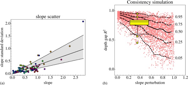
Figure 15.

(a) The standard deviations of the slope (the slope is the tangent of the slant) as a function of the magnitude of the slopes for all observers (color indicates observers). The line indicates a Weber law with Weber fraction 0.35 (median value); the range between the dashed lines shows the interquartile range (0.22–0.55). The lowest value of the slope standard deviation is 0.032. (b) The result of a simulation that finds the coefficient of variation between the estimated and observed depth gaps as a function of the Weber fraction. A ‘true’ geometry of 200 times the first principal component (see text) was used, which is roughly the median configuration. The simulation is composed of 5000 runs. Quartiles and 0.05 and 0.95 quantiles were calculated in 0.1 width moving windows. The yellow whisker dot plot indicates the range of empirical coefficients of variation; shown are the quartiles, 5% and 95% quantiles, and the outliers. The width suggests the uncertainty in the Weber fraction. As the interquartile regions overlap, and the range of outliers is similar, we conclude that the observed Weber fraction explains the coefficients of variation encountered in the empirical data.