Pictorial depth probed through relative sizes

Abstract

In the physical environment familiar size is an effective depth cue because the distance from the eye to an object equals the ratio of its physical size to its angular extent in the visual field. Such simple geometrical relations do not apply to pictorial space, since the eye itself is not in pictorial space, and consequently the notion “distance from the eye” is meaningless. Nevertheless, relative size in the picture plane is often used by visual artists to suggest depth differences. The depth domain has no natural origin, nor a natural unit; thus only ratios of depth differences could have an invariant significance. We investigate whether the pictorial relative size cue yields coherent depth structures in pictorial spaces. Specifically, we measure the depth differences for all pairs of points in a 20-point configuration in pictorial space, and we account for these observations through 19 independent parameters (the depths of the points modulo an arbitrary offset), with no meaningful residuals. We discuss a simple formal framework that allows one to handle individual differences. We also compare the depth scale obtained by way of this method with depth scales obtained in totally different ways, finding generally good agreement.

1. Introduction

“Familiar size” is perhaps the best known depth cue (Berkeley 1709). It is the basis of stadimetry,⁽¹⁾ which has been—and occasionally still is—of military importance in range estimates for gunnery. When the absolute size (as in the case of people) is not available, one may still use the size cue whenever multiple instances of some kind of object are simultaneously detected. In this case the size cue yields ratios of distances. It suffices that the objects are merely statistically similar, common instances are trees or barns in a landscape. This can be further generalized to certain cases of the “texture gradient cue”⁽²⁾ and so forth. The size cue is discussed in virtually any introductory textbook on vision (Gibson 1950; Palmer 1999).

The size cue is well understood for the case of vision in physical space. It depends immediately on range—that is, distance reckoned from the eye.

It is rarely recognized that the size cue cannot pertain (at least not in an immediate way) to pictorial space. The eye is not in pictorial space (Koenderink and van Doornl 2008), thus there is no such a thing as “range”. Yet painters often use relative size as a cue to pictorial depth (Gombrich 1960). Apparently the classical “size cue” of vision science (related to stadimetry, etc), and the use of relative size as a pictorial depth cue (as evident from the painter's practice), are two distinct things. This paper, in contradistinction to the bulk of the vision literature, deals specifically with the latter case.

That human observers are sensitive to the size cue as a pictorial cue seems indeed likely from its frequent use by visual artists. The pictorial size cue often works even in the absence of perspective in the formal sense (Figure 1). Cases where it seems hardly used include such pictures as Japanese woodcuts of interiors before the introduction of Western perspectivism (Lane 1978). An interesting example is Thebaid, attributed to Gherardo Starnina, painted in 1410. In such pictures things do not change in pictorial size as they recede, with castles in the foreground smaller than huts in the background, people larger than bridges, etc (see Figure 1a). Nevertheless, such pictures still have a well developed pictorial space due to other cues. The same holds for early Persian miniatures (Kianush 1998). In such renderings depth is mainly generated by mutual overlap (generating a depth order), and height in the picture plane (generating a continuous scale). These are instances where the size cue remains simply ineffective.

Figure 1.

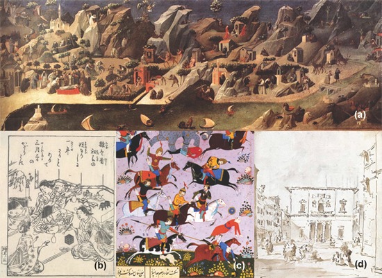
(a) Thebaid, a landscape painting attributed to Gherardo Starnino (http://www.independent.co.uk/arts-entertainment/art/great-works/starnina-gherardo-attribthebaid-1410-934885.html). Painting belonging to the collection of the Uffizi Gallery, Florence, Italy; http://www.uffizi.org/. (b) a Japanese woodcut (the Japanese woodcut comes from a page from an 18th-century printed book by Nishikawa Sukenobu depicting Hina Matsuri (Doll's Festival) events). (c) A Persian miniature (http://micheleroohani.com/blog/2009/06/16/iran-better-days-will-come%5CT1%5Ctextemdash%20though-not-yet/). (d) Pen drawing by Francesco Guardi. View of La Fenice, Venice (recto), Courtyard Interior (verso), Francesco Guardi. Pen and brown ink and wash (recto), pen and brown ink and grey wash (verso), h: 25.6 × w: 22.2 cm/h: 10.1 × w: 8.7 in.

Cases where the size cue is intentionally confusing are common enough in Western art (see Figure 2). Examples include such diverse instances as Goya's Giant, and Mel Ramos' pop art pictures. The “giant” sits upon the horizon (as implied by overlap cues) and is thus miles away. Its apparent size must thus be due to gigantic physical size. A similar case is Klinger's tiger in the mountains. Here we directly compare the pictorial size of the tiger and features of the landscape, resulting in the impression of a gigantic animal. In Mel Ramos' Lola Cola (a picture in the intentionally doubtful taste that is typical of “pop art”) the nude lady and the coke bottle are evidently at about the same depths. Yet the familiar size cue puts the bottle far in front of the pin up, yielding a stimulating tension. What makes such cases of artistic interest (from a cognitive perspective these are merely poor jokes) is that the viewer's visual awareness is influenced directly, that is to say, before cognition proper kicks in.

Figure 2.

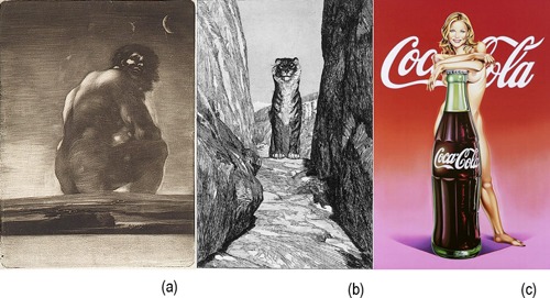
(a) Goya's Giant, Francisco de Goya y Lucientes (Spanish, 1746–1828), 1818. Burnished aquatint, 1st state. (b) Klinger's First Future (Max Klinger (1857–1920), Erste Zukunft (From the series Eva und die Zukunft, 1880.) Etching with aquatint: 14 3/16 × 9 1/4 in (36 × 23.5 cm). (c) Mel Ramos's Lola Cola. Mel Ramos (born 1935), Lola Cola #4 (Michelle Pfeiffer), 2004. Lithograph, 34.5 × 23 in. The bottle is, of course, the famous 1916 design, reputedly modeled after the figure of Mae West.

Different from the theory of the size cue in physical space, there is currently no theory of the size cue in pictorial space. Nor are there operational methods or quantitative studies. We propose both theory and operational methods. Our aim is to investigate to what extent the pictorial size cues lead to coherent results. (Coherency to be suitably defined in some specific way elaborated below.) The research is necessarily of an exploratory, preliminary nature, given that we are charting unknown territory here.

It is perhaps not superfluous to remind the reader that there exist distinct concepts of “picture”. In one (rather extreme) view a picture is much like a window (Alberti 1972; da Vinci 1888; Gibson 1971). This implies that the viewer is related to the pictorial content in the sense that the viewer is part of the pictorial space. In order for this to happen, the picture has to be in perfect linear perspective and the (single) eye has to be at the center of projection. This case is often approximated in the laboratory (in many conventional setups,⁽³⁾ as well as in “virtual reality” displays nowadays), or through the help of optical devices such as peephole shows or special viewers.⁽⁴⁾ In the more common understanding of the term a picture is simply a planar surface covered with pigments in a certain simultaneous order.⁽⁵⁾ In this case the viewer is not likely to have the eye at the perspective center; nor is it of any interest to attempt to achieve this, since there not necessarily is a perspective center.⁽⁶⁾ In modern Western art, and most of non-Western art, the linear perspective of the European renaissance period (Alberti 1972) is not used at all.

Cases akin to virtual reality fit into the standard accounts of the size cue in physical space. Therefore these are not related to the current topic.

In the case of true “pictorial” perception the viewer is not geometrically related to the pictorial content; the eye is not located in pictorial space at all. This has the immediate consequence that pictorial objects have no distance to the eye; the concept remains undefined. In visual awareness, pictorial objects often have a quality known as depth, though. This is the case regarded here.

Depth and distance are categorically different entities (Figure 3). For instance, distance is a non-negative quantity, with an obvious origin: distance zero is where the eye is. Thus the range, or distance domain, is the real half-line. In contradistinction, depth has no obvious origin. The eye is not even in pictorial space; it is not at any particular depth at all. In fact, absolute depth is a non-entity. Only depth differences can (perhaps) be ascribed some meaning. Consequently, the depth domain is (at best) the full affine real line.⁽⁷⁾ In many cases the depth domain may have even less structure.

Figure 3.

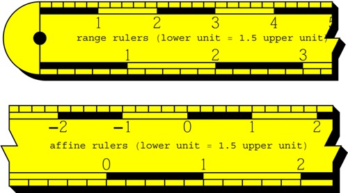
At top an example of a range scale. The upper and lower scale are equivalent, although the units are different. This case can be arbitrarily prolonged towards the right, but it “stops” at the origin at left. The origin is at the black dot (a hole), which can be used to pin the ruler with a nail. If you are interested in range ratios, either scale will do; you are guaranteed to obtain the same result. At bottom an example of an affine scale. The upper and lower scale are again equivalent, although in this case both the origins and the units are different. This scale can be arbitrarily prolonged in either direction. There is no “natural origin”. If you are interested in the bisection of line segments, or the ratio of segment lengths, for line segments at any location, either scale will do. You are guaranteed to obtain the same result.

In typical cases of pictorial vision there cannot exist any causal or functional relation between distance and depth, for the simple reason that distance (or range) remains undefined. In Appendix A we consider speculative relations between range in physical space and depth in “visual space” (ie, the subjective equivalent of physical space). This might be useful in cases where the relative size cue would be used in real scenes, or calibrated pictures. The case of pictorial space is categorically different from that of visual space because there is no immediate relation to a physical space. Below we consider it using a few general arguments.

In Figure 4a we consider the very simple case of two visual objects that are identical except for location and size. The larger one (1) looks nearer than the smaller one (2). In Figure 4b we repeat configuration (a) but on an overall smaller scale. In order to construct a numerical scale for depth, we evidently want to let the depth of (a)1 be smaller than that of (b)2, and likewise the depth of (b)1 be smaller than that of (b)2. As a desirable constraint we want the depth difference to depend only upon the ratio of sizes (diameter of (a)1 relative to diameter of (a)2, and diameter of (b)1 relative to diameter of (b)2). Moreover, we want the depth difference to be independent of the absolute size of the objects. Thus the depth differences (a)1 – (a)2 and (b)1 – (b)2 should be equal in the case of the example. Another desirable objective is that the scale be additive. That is to say, one would like to impose the constraint that the depth difference (c)1 – (c)3 be equal to the sum of the depth differences (c)1 – (c)2 and (c)2 – (c)3. It is immediate to show that this implies that the depth difference should be defined as the logarithm of the ratio of the sizes.

Figure 4.

(a) Two pictorial objects of different size. When superimposed over the picture, object 1 looks less distant than object 2. (b) Again, two pictorial objects of different size, object 1 looking less distant than object 2. In this case picture (b) is a scaled version of picture (a). (c) Three pictorial objects, 1 the largest, 3 the smallest. Object 1 looks closer than object 2, which again looks closer than object 3.

Notice that this relation reflects only the properties of the numerical depth scale that we impose on the judgment of relative sizes and has nothing whatsoever to do with the elementary geometry of the size cue in physical space. This is indeed necessary, because there exists no equivalence of “range” (that is distance reckoned from the eye), because the eye is not in pictorial space. (The eye does not see itself.)

To impose the two constraints of independence of absolute size and additivity is natural. The independence of absolute size is an obvious requirement, as seen in Figure 5. The depth difference between the super-objects (a) and (b) should be the same as that between the sub-objects (a)1 and (b)1, even though (a) – (b) and (a)1 – (b)1 differ in scale by a factor of two. The additivity constraint is natural because the depth scale has neither a natural origin, nor a natural unit. The constraints make it into an affine line: We only assign depth differences through the log-ratio of sizes (a single item cannot be assigned a depth), and the base of the logarithm remains arbitrary, the depth difference unit is determined only up to some arbitrary (though positive) common factor.

Figure 5.

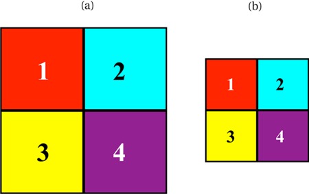
(a) an object composed of four smaller sub-objects; (b) the same configuration at smaller scale. The depth difference between the super-objects (a) and (b) should equal the depth difference between sub-objects such as (a)1 and (b)1.

One has to assume that different observers will yield depth scales that mutually differ by arbitrary (though not depth reversing) affine transformations. They might use the upper and lower scales of the ruler shown in Figure 3, for instance.

As we will show in this paper, simple methods allow one to perform rather strong tests on the consistency of the scale obtained for general point configurations in pictorial space for a single observer, as well as the consistency of the scales obtained for different observers of the same picture.

We propose to put the relative size cue to good use as a depth probing tool, by showing a pair of obviously identical objects at different locations (like those depicted in Figure 4) and requiring the viewer to adjust their relative pictorial sizes such as to look equal size in pictorial space. Repeating this for many pairs should allow us to probe the space for depth.

The aim of the paper is to explore the viability of this method and to find its limits and general characteristics. Since we have implemented a number of different methods to probe pictorial space in the past, we are in a position to address the mutual coherence of such methods. This goes some way towards the solution of the question as to whether the concept of pictorial space itself may be ascribed a useful meaning.

2. Method

In this paper we propose to turn the relative size cue into an effective probe of the structure of pictorial space. We concentrate on the generic case of pictorial perception, rather than the rather singular “window” mode in which the eye position has a relation to the picture geometry.

In setting up the method, one encounters some generic problems involved with any probing of pictorial space by means of localized probes. We have extensive experience with these problems, and have discussed them on frequent occasions. In a nutshell, here is how to introduce any probe into pictorial space.

To start with, notice that pictorial space is a mental entity, whereas the picture plane is a physical entity. A picture is a planar surface covered with pigments in some simultaneous order. When looking into, as opposed to at, a picture, visual awareness breaks through the picture plane so to speak, and conjures up a three-dimensional spatial organization to the mind. This is a spontaneous, effortless process, the awareness simply happens to the observer, much like sneezing. This “presentation” is proto-cognitive in that the observer has little or no control over it. Prolonged looking, typically accompanied by voluntary and involuntary fixations, is apt to lead to a series of mutually similar but distinct presentations. Each single presentation lasts only a moment (Brown 2002). In having such presentations, the observer experiences the simultaneous order of pigments on the picture surface as pictorial space. Putting a physical mark on the picture surface often results in the appearance of something novel in pictorial space. This is, of course, exactly what happens when a painter puts another touch on the surface.

Two things happen simultaneously when the painter touches the canvas with the loaded brush. Some paint is added to the surface, and something changes in pictorial space. The painter manipulates pictorial space at the same time as the physical surface is being manipulated. Some painters feel they are primarily working on the canvas, others that they are working on the image. Both agree that they (cannot help but) work on both. Putting a spot of dark paint on the surface of a portrait thus may result in the appearance of a “beauty spot” or “freckle” on the pictorial skin. The mark travels into depth until it comes to a halt at the nearest pictorial surface on which it adheres. In putting the mark on the canvas, one may feel that one touches the cheek. Phenomenologically, the experience is not that different from feeling the head of a screw at the end of a screwdriver, or the paper surface at the tip of one's pen.

We exploit this phenomenon to put probes into well defined locations in pictorial space. The process is really simple, one just superimposes a physical mark on the picture surface. If done right, this results in the appearance of a pictorial mark on some pictorial surface, or clinging to some pictorial object. In order to do this right, one should select a suitable location, and a suitable mark. For instance, a dark spot in the blue sky may appear as a pictorial bird (with poorly defined depth) or will not “cross the surface” and merely appear as a superficial smudge, not related to pictorial space at all. Again, a symbol from some font may fail to adhere to a cheek, but may well adhere to a fronto-parallel wall, and so forth. In practice, we localize suitable marks at well defined, smallish pictorial objects (Figure 6). Typically, a mark will “attach” and be at a well defined pictorial location.

Figure 6.

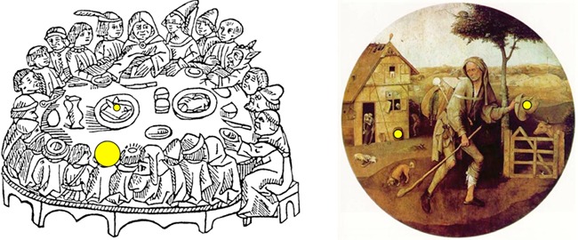
At left medieval wood print with two superimposed marks. The two marks are geometrically similar, but of different size. Notice that the lower one “attaches” to one of the persons sitting at front, whereas the higher one looks attached to a swine head on the table. Are these objects of the same size in pictorial space (as different from the picture plane)? It will depend upon the observer. The higher one looks too small to us. Notice that the woodcut is an example where the artist did not use the relative size cue for depth. In the painting at right the relative size cue is important. The two marks are equally large in the pictorial plane. The farther one looks too large to us.

In running the sessions, we make sure that the observers report to experience the marks in pictorial space. It is throughout conceivable to encounter observers for which this would fail to be the case. However, we still have yet to meet such a case. If we do, then we would have to give up for that person. There is no way to force people to experience pictorial spaces; we simply have to rely on their proto-awareness.

In our present implementation the marks are small semitransparent yellowish circular blobs of variable diameter, outlined with a dark hairline (much as in Figure 6 but more transparent). Such marks appear either as fronto-parallel disks or spheres in pictorial space. Even if of a single physical size, they may appear of rather different pictorial sizes. This works similarly to “Emmert's Law” (Emmert 1881): when introduced in the background, they will appear larger than when introduced into the foreground. Given two of such marks, the question of whether these appear as pictorially identical objects (that is, of the same size) makes solid visual sense.

In order to forge a method of depth difference measurement, we grant the observer control over the relative size of the two marks, always keeping the geometrical mean of their diameters constant. The task itself is a simple one: The observer has to adjust the relative sizes such that the two objects look the same size. We then cheerfully invoke the theory discussed in the introduction and interpret the logarithm of the size ratio accepted by the observer as the depth difference. Of course, this should be interpreted only as our operational definition of the depth difference. From this perspective, such a definition in no way depends upon the theory, which was used only as a heuristic device to come up with the definition. Whether such a definition makes sense at all then becomes an empirical issue, and this is what the present paper centers upon.

A strong test of the viability of the method requires one to study many pairs from some extended point configuration in pictorial space. There are many more pairs than points, since the number of pairs grows quadratically with the number of points. Any point participates in many pairs. Thus the issue of mutual coherence of a set of depth differences is easily addressed empirically.

There are a number of limitations of any such a method that are already obvious a priori. A major one involves the depths of very distant points. For large depth differences (for instance, those involving points on the horizon of a landscape) the size ratios are likely to become very large, and instead of a well-defined numerical value, one finds that the observer decides to be satisfied with “large enough.” In the present experiment we include a (small) number of instances in which the task becomes ill-defined for this reason. In the final analysis we have taken account of the special nature of these cases.

Another problem is due to the fact that we do not consider well-calibrated, “window-like” pictures. As the theory discussed in the introduction suggests, this means that the depth differences obtained in an experiment will suffer from unknown scaling factors and offsets. Since such scaling factors are not (ill-)specified by the pictorial cues, one has to assume that it will be idiosyncratic, with the result that the depths obtained for different observers will at best be scaled copies of each other. This will affect the type of analysis that might sensibly be applied to the empirical results.

We address such problems in subsequent sections of the paper.

2.1. Participants

Participants were volunteers from the Laboratory of Experimental Psychology at the University of Leuven and the authors. No observer, including the authors, had any prior experience with the method. Only the authors had given it some thought before embarking on the trials. All observers had seen the stimulus picture before, since they participated also in past (rather different) experiments involving this figure.

Ages varied from early twenties to late sixties. Both genders were represented (three females, four males). Familiarity with the visual arts ranged from scant to extensive.

Each observer completed three full sessions. A full session included many trials, each ordered pair of locations being presented once. The pairs were presented in random order for each session.

2.2. Procedure

The stimulus picture was a copy of a wash drawing by Francesco Guardi⁸ by Anne-Sophie Bonno.⁹ The picture represents a “capriccio,” that is an imaginary landscape, based on the generic Veneto environment of the 18th century. Thus no such thing as “the ground truth” is available. The landscape is of the standard type encountered in Guardi's time, with clearly delineated foreground, middle ground, and background. Such constructions still work well for present day observers, even those with little or no experience with the visual arts. Depth cues include height in the picture, local tonal value, local strength of line, overlap, increasing generalization of details with depth, and familiar size (persons, boats, houses). Of course, these cues tend to correlate strongly with each other.

The picture was presented on a DELL U2410f monitor, 1920 × 1200 pixels LCD screen, and viewed from a distance of 78 cm. The room was semi-dark, all of the light being due to the display. This was just enough for the observers to find their way around the keyboard. This implies that the frame of the display was (dimly) visible and that the observers were fully aware of the fact that they were looking at a flat, rectangular screen.

Viewing was monocular with the dominant eye, the other eye being patched or closed. Viewing was through a 4 cm circular aperture at fixed position, the head being stabilized by a chin and forehead rest. The picture measured 36.9 deg (width) by 27.4 deg of visual angle; thus the foreshortening factor at the left and right edges was 0.951, within 5% from unity, which was our design objective.

At this distance the available physiological depth cues are expected to be largely inactive. Binocular disparity is not available due to monocular viewing; thus only monocular parallax and accommodation might be expected to matter. The accommodation difference between the center and the left or right edge of the picture is less than a tenth of a diopter, which is subthreshold. The monocular parallax is 17 minutes of arc for an eye turn of 18 deg (half the diameter of the stimulus). The difference in monocular parallax between center and edge of the picture is less than a minute of arc, which is subthreshold. Thus monocular parallax yields a uniform translation over about 17 minutes of arc for an eye movement subtending about 18 deg, which is again subthreshold. Thus the physiological depth cues signal either a scene at large distance or a flattish surface. Since observers appear to localize the scene as near to the picture surface (a bit like the view in an aquarium or terrarium), the physiological cues may be expected to contribute a weak tendency to flatness, something that has been verified in other settings (Koenderink et al 1994).

A session consists of a series of similar trials, presented in random order. Each trial starts with a view of the picture over which two yellowish, circular disks, both outlined with a black hairline had been superimposed. The observer uses a computer keyboard to control the relative size of the disks in 1% intervals. The left and right arrow keys each change the relative sizes, though in opposite directions. Thus the observer has to rely on vision to know the relative sizes, the interface yielding no cue. The observer takes arbitrary time to adjust the relative size until the two disks appear as a pair of identical spherical objects in pictorial space. When satisfied, the observer actuates the space bar, which initiates the next trial.

At the close of the session results are sorted, and relative sizes converted to depth differences by taking the logarithm of the ratio. The set of all depth differences is then converted into a much smaller set of relative depth values. These depth values are normalized by constraining their average to equal zero. Apart from the list of depth values, the root mean square deviation between the explained and the observed depth differences is collected as a datum.

3. Results

Observers find the task intuitive, and generally fun to do. It is easily possible to handle point configurations comprised of about 20 points in sessions of about an hour. Notice that a point configuration of N = 20 points implies ½N(N − 1) = 190 ordered pairs, and thus as many trials. The size ratios are converted into 190 depth differences, and a standard procedure (involving the pseudoinverse [Penrose and Todd 1956] of the matrix defined by the least squares problem) is run to find the 20 depth values, always under the constraint that the average depth equals zero. From the 20 depth values we find 190 “explained” depth differences, and the standard deviation of the mismatches from the actually observed depth difference values is taken as a measure of the coherence of the result. We repeat this to obtain three independent sessions from each observer. From this we attempt to determine the standard deviation in the observed depth differences.

The fiducial locations are shown in Figure 7 and Figure 8, with a typical result for one session. Apparently the method “works” at least in principle in that it yields a three-dimensional point configuration. Such configurations turn out to be at least roughly similar for all observers and for the repeated sessions of a single observer. Moreover, the configuration makes sense in that one obtains a clear ordering of points in the foreground, the middle ground, and the background.

Figure 7.

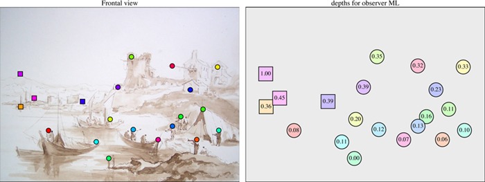
At left the stimulus picture with the 20 fiducial locations indicated. The points indicated with square marks are in the far range. The points are labeled by hue. At right the depths from one session of observer ML. In protect Figure 8 the same data are represented in three-dimensional pictorial space. Again, the points are labeled by hue. For the sake of concise rendering the numerical values have been normalized on the range of zero to one, and coarse-grained to two significant figures.

Figure 8.

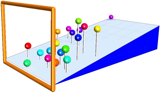
The same data as in protect Figure 7 right. The depth dimension has been arbitrarily scaled so as to render the picture clear. The sloping plane is the ground-plane (water surface) estimated from the data. The orange frame is the picture frame. It is as if observer ML were looking into a classical stage proscenium. The hues correspond to those defined in protect Figure 7 left.

A more precise study of such data can be based on scatter plots of depths for corresponding fiducial locations. In Figure 9a we show such scatter plots for the three sessions of a single observer (ML) over either the full or the near range, and in Figure 10a the means of the three sessions of each observer against the mean over all observers, again either over the full or the near range. What is evident is that the correlations are very high, but that the slopes of the regression lines are rather variable. This complicates the analysis; for instance, one may not simply calculate the standard deviations for repeated sessions because the results apparently show systematic variations. The reason for the variability of the slopes is no doubt the fact that depth differences are only defined up to some unknown scaling factor. One has no reason to consider this scaling factor to be anything but fully idiosyncratic. Apparently, it varies between observers and even for the repeated sessions of a single observer. Since sessions were completed in single sittings, one may perhaps expect the factors to be approximately constant (though unknown) for given sessions. Such variations can be removed by suitable scalings (see next section, and Figure 9b and Figure 10b). After such scaling the remaining scatter is of interest.

Figure 9.

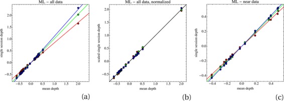
(a) A scatter plot of the three sessions of observer ML based on all data. Depths of each individual session are plotted against the mean of the three sessions. The regression lines for the three sessions are clearly distinct. (b) A scatterplot containing the same data, but after applying affine transformations that align the regression lines. This removes the idiosyncratic scalings. (c) A scatter plot of the near field data alone. These are the same data as in the left plot, but because the far range data are removed, the means are, of course, different.

Figure 10.

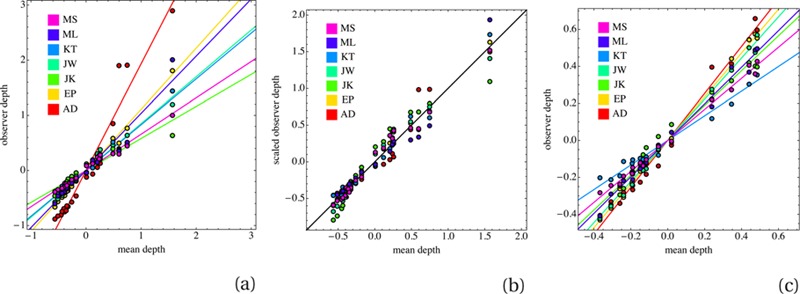
(a) A scatter plot of the means of the three sessions of all observers, based on all data. Depths of each observer are plotted against the mean over all observers and all sessions. The regression lines for the observers are clearly distinct. (b) A scatterplot containing the same data, but after applying affine transformations that align the regression lines. This removes the idiosyncratic scalings. (c) A scatter plot of the near field data alone. These are the same data as in the left plot, but because the far range data are removed, the means are of course different.

For the single observer ML in the near range (results shown in Figure 9c) we find that the remaining scatter is 0.017 (standard deviation of corrected depth differences), whereas the total depth range is 0.904. Thus this observer might be said to resolve about 55 depth layers.⁽¹⁰⁾ For all observers one has the results shown in Table 1. The rank order correlation between the depth ranges and the number of resolved depth layers is not significant. Apparently, depth range and resolution are largely independent. Both vary by as much as a factor of two over our observers. (More details can be found in the Analysis below.)

Table 1. The standard deviations in the depth settings, corrected for idiosyncratic scalings, the depth range, and the number of resolved depth layers in the near range, for all observers.

Observer	Standard deviation	Range	Layers
AD	0.048	1.07	22.2
EP	0.041	1.01	24.5
JK	0.022	0.83	36.9
JW	0.020	0.99	50.2
KT	0.020	0.57	28.6
ML	0.017	0.90	54.5
MS	0.023	0.71	30.5

The scaling factors differ both over sessions of a single observer and over the mean data of all observers. The scaling factors for the observers differ by as much as a factor of 3.33 as evaluated over all data, 1.91 as evaluated over the near range, and 5.23 as evaluated over the far data. An overview of the magnitudes is given in Figure 11.

Figure 11.

The scaling factors encountered in the experiment. (a) The scaling factors of the full data against the grand mean. (b) The scaling factors for the near field data against the mean of all near field data. (c) The scaling factors for the far field data against the mean of all far field data. For each observer we show the median and the extremes.

The mutual correlations of the mean depths over three sessions for all observers are given in Table 2. The correlations are all very high; the lowest value for the full range is 0.873. For the near range it is 0.958, and for the far range 0.888.

Table 2. The mutual correlations of the mean depths (over three sessions) of all observers. The table at top gives the correlations for the full data; the table at center, those for the near range; and the table at bottom, those for the far range.

	EP	JK	JW	KT	ML	MS
AD	0.949	0.895	0.923	0.946	0.913	0.930
EP		0.939	0.985	0.992	0.981	0.990
JK			0.975	0.911	0.873	0.960
JW				0.966	0.948	0.995
KT					0.981	0.977
ML						0.965
AD	0.987	0.969	0.985	0.987	0.982	0.990
EP		0.981	0.994	0.985	0.994	0.992
JK			0.983	0.958	0.979	0.979
JW				0.981	0.989	0.995
KT					0.980	0.987
ML						0.984
AD	0.915	0.948	0.907	0.888	0.938	0.927
EP		0.975	0.992	0.994	0.985	0.998
JK			0.989	0.945	0.947	0.986
JW				0.974	0.958	0.996
KT					0.988	0.986
ML						0.979

The overall result is that observers show very similar results in the near range, whereas they differ rather markedly in the far range. The differences involve idiosyncratic scalings, for the correlations are high, both in the near and in the far range.

4. Analysis

In order to compare a number of sessions, we first find the mean over all sessions. Then we perform a linear regression of each session against this mean. This yields a scaling factor (slope of the regression line) for each session. Next we perform the inverse scaling on the results of each session. As a result the three sessions become immediately comparable (Figure 9b). Once the systematic deviations are removed, one is left with only the random scatter of the data. This allows one to estimate the standard deviation in individual depth differences. This standard deviation may be compared with the total depth range so as to yield a measure of the depth resolution—that is, the number of depth slices that the observer distinguishes in the pictorial space (Table 1).

Another important measure involves the internal consistency of the three-dimensional configuration. For N fiducial points one observes ½N(N − 1) depth differences, whereas these observations are accounted for by N − 1 degrees of freedom, namely the N depth values under the constraint that the average depth is identically zero. These depth values imply depth differences, which will differ from the observed ones. The standard deviation of these mismatches is a measure for the internal consistency of the three-dimensional configuration. This standard deviation should be comparable to the scatter—that is, the standard deviation for repeated settings (as discussed above) divided by the square root of N − 1 (because each point is involved in N − 1comparisons). In case it is, the method may be declared to yield consistent results; in a sense it is a sign of the very existence of pictorial space as operationalized by the method.

In Figure 12 we show overall results. From a Monte Carlo simulation we expect the mismatches (see previous paragraph) to be about 0.67 times the scatter. Our data are too noisy to check this more precisely. The conclusion is that the mismatches are accounted for by the scatter in repeated sessions. Apparently, the method yields coherent geometrical data. We consider this to be an important finding of the study.

Figure 12.

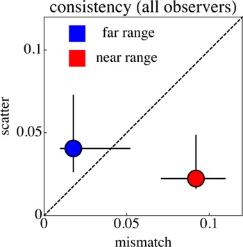
The standard deviation in the “mismatches” versus the “scatter,” which is the standard deviation in the depth differences from the three repeated sessions divided by the square root of N−1 for all observers. The lines show the total range, the dots the median values. The data have been split into the near and the far ranges.

As a final point we consider the question of whether the presence of human figures in Guardi's capriccio might have rendered the task virtually trivial, that is to say, a straightforward application of stadimetry by the observers. We believe this objection to be pointless for the following reasons. There are seven fiducial locations attached to human figures, mainly heads. This implies 21 trials, only 11.1% of the total number of trials (190). We checked whether these trials were especially precise; this was not the case. We also measured the heights of the figures (in pixels) and calculated the corresponding stadimetric depth differences. For one subject (we discuss observer ML here, but the result generalizes to all participants) the observed depth differences correlate only very weakly with the stadimetrically predicted depth differences. The correlations are very low as compared with other levels reported in this study. In Figure 13a one notices an appreciable scatter. We conclude that there is no particular reason to assume that the stadimetric cue played an important role in the behavior of the observer. Other cues, for instance, height in the picture plane (Figure 13b) correlate just as well, if not better, with the observations.

Figure 13.

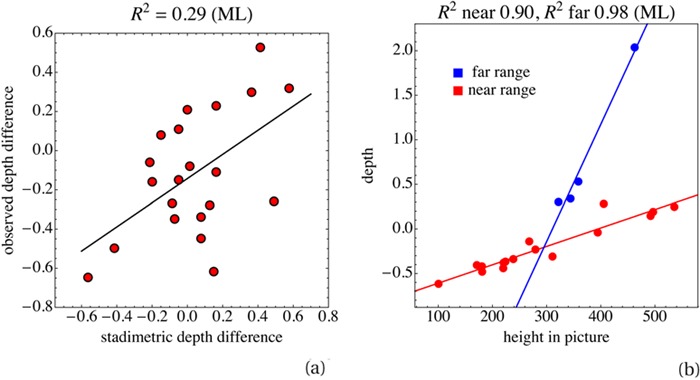
(a) Scatterplot of the observed depth differences (by observer ML) plotted against the depth differences predicted from stadimetry. Only depth differences between locations at pictorial figures are considered. (b) Scatterplot of the depth of a session of observer ML against heights in the picture plane (heights expressed in pixels).

In Figure 13b we have treated the near and far ranges separately. Both evidently correlate strongly with height in the picture plane, although the slopes of the regression lines are very different. All observers correlate highly with the height cue, but the difference between near and far ranges appears to be idiosyncratic.

5. Comparison with prior results

The data from these relative size measurements may be compared with results obtained by way of different methods to probe the geometrical structure of pictorial space. This is possible because the observers in the present task also participated in prior experiments involving the same stimulus picture (of course, this was the very reason for the choice of both observers and stimulus picture) and because depth can be used as a “common currency.” We consider two alternative probes, namely the method of pairwise depth comparison (van Doorn et al 2011) and a method of exocentric pointing in pictorial space (Wagemans et al 2011). For both methods we use the final data per subject. Further details can be found in the original papers.

The method of pairwise depth comparison yields only an ordinal depth scale. Of course, one expects perceived depth order to correlate very well with the sign of the depth difference. Only in the case of depth differences that are very small in an absolute sense would one expect occasional, random violations. Indeed, the depth scale established through size comparisons may be expected to yield a metrical calibration of the ordinal scale obtained through pairwise comparison. We check this in two ways, first we find the Kendall rank order correlation; then we prepare a scatter plot of depth order against depth. This latter plot is expected to be monotonic throughout. These expectations are fully borne out, as shown in Figure 14a. The Kendall rank order correlations have been collected in Table 3.

Figure 14.

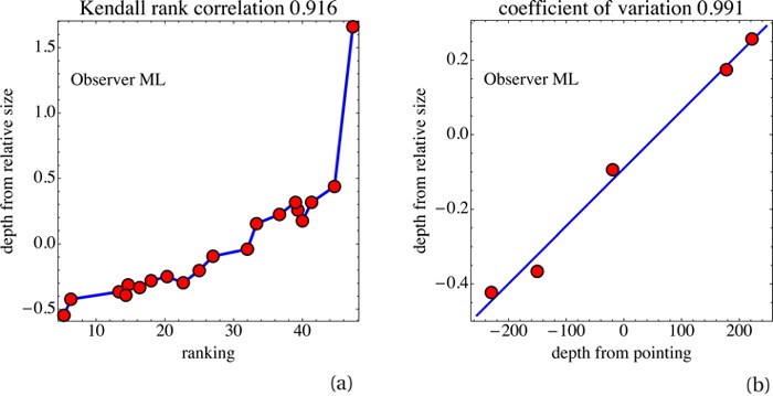
(a) Scatter plot of the ranking (depth order) from pairwise comparison against depth from relative size for observer ML (session 1). Notice only incidental small deviations from monotonicity. The rankings are for a greater number of fiducial points (about fifty) than used in the present experiment, hence the scale. (b) Scatterplot of the depth from a pointing task (expressed in pixels) against depth from relative size for observer ML (session 1). The pointing depths are for a lesser number of fiducial points (five) than used in the present experiment. The correlation is very high.

Table 3. The median Kendall rank order correlation of the depths from the relative size cue with the rank order determined from pairwise comparison, and the median of the correlation of the depths from the relative size cue with the depths from an exocentric pointing task.

Observer	Pointing depths	Rand order
AD	0.978	0.947
EP	0.932	0.926
JK	0.991	0.979
JW	0.871	0.926
KT	0.986	0.850
ML	0.968	0.937
MS	0.981	0.916

The rank order correlations are throughout high (median 0.926, range 0.850–0.979), and deviations from monotonicity are rare.

The number of resolved depth slices as determined by the method of pairwise comparison is similar to that obtained from the present method. In this respect the methods completely agree.

The method of exocentric pointing in pictorial space is rather more interesting than a mere pairwise comparison because it yields a depth scale by means of a completely different paradigm, making the comparison a challenging one. In this method one sets the observer to the task of adjusting the spatial attitude of a pointer (rendered as a solid arrow) so as to point to a target (rendered as a roughly spherical solid object). This (like the relative size task) involves a pair of fiducial locations for each trial. However, whereas we may use unordered pairs in the relative size task, we have to use ordered pairs in the exocentric pointing task. The reason is that observers “point by arcs”—that is to say, the pointing directions from A to B and from B to A turn out to fail to be collinear. This implies a doubling of the number of trials. In practice, the pointing method allows one to use up to about 10 fiducial points if sessions are to be limited to about an hour. In a prior experiment we used 5 fiducial points, a subset of the 20 fiducial points used in the present experiment. The exocentric pointing method yields a set of depth values for the fiducial points, up to a common offset. In practice, we constrain the average depth to be zero. The depths from pointing may be immediately compared with those from the relative size task. Because they involve very different geometrical relations, this yields a strong check on the internal consistency, or perhaps the very existence, of pictorial space (Figure 15).

Figure 15.

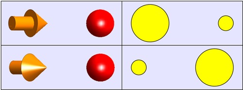
The mutual depth relation between two fiducial points from the perspective of exocentric pointing (left) and the relative size cue (right). Because these methods involve very different geometrical relations, an agreement between results obtained with these methods goes some way to show that pictorial space has an existence apart from any specific manner of prospecting it. In the top row the left item “looks closer” in the bottom row the right item “looks closer.” The reason why is, of course, very different for the left and for the right column.

We find that depths from the relative size and the exocentric pointing method correlate very well for all participants in the experiments (figure 14b and Table 3). Correlations are generally in the 0.9 range (median value 0.978, range 0.871–0.991). In both cases (relative size cue and exocentric pointing task) the depth values are only determined up to some idiosyncratic scaling factor.

In the case of the exocentric pointing method we reported depth ranges differing by as much as a factor of four; in the present case we find similar differences. It is obviously of considerable interest to see whether these differences are essentially unpredictable or whether they are specific to individuals. There is indeed some reason to expect the latter, because the factor varies rather less over the trials of any given individual than over the group of participants. This has been found for both methods. We explore this issue in the scatter plot presented in Figure 16.

Figure 16.

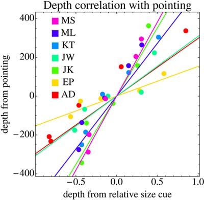
Combined scatterplot for all observers of mean depths from the relative size cue task and the depths from an exocentric pointing task.

The magnitude of the depths in Figure 16 might appear surprising at first blush. The depths for the exocentric pointing task are expressed in terms of pixels (as measured in the picture plane), for this task this is a natural measure. We may attempt to bring the present depth values in the same format by noticing that the horizontal extent of the picture subtends 36.9 deg, that is 0.644 radians, whereas the picture subtends 1024 times 768 pixels. Using the two-dimensional model discussed in the introduction as a heuristic, we might scale the depth values by 1024/0.644. Consider a depth range of (–0.5, +0.5); then we obtain for the scaled range −795 to +795. This is indeed much closer to the depth range of the exocentric pointing results. Apparently, the heuristic works quite well.

The slopes of the linear fits to the scatterplots in Figure 16 differ by a factor of almost five (4.97). Apparently, there is hardly any relation between the depth ranges obtained through the two methods.

6. Discussion

In this paper we considered the pictorial relative size cue. In the case of pictorial perception the eye is not related to the geometry of the pictorial content; thus there is no notion of a “range”, that is, “distance from the eye”. The conventional theory of the size cue, which is highly developed, does not apply; nor does the work relate strongly to the large body of empirical studies involving the size cue in physical space. (See Gibson 1950; Palmer 1999.)

Here we introduced a novel operationalization of depth in pictorial space based upon the relative size cue. We also compared the results to metrical or ordinal depth scales obtained from alternative operationalizations. Each of these methods allows for an independent check of the geometrical coherence of that method, and taken together, one obtains a number of independent checks on the mutual coherence of pictorial space as revealed by different methods of prospecting it. This is to be considered most important, as it bears on the basic issue of whether the concept of a “pictorial space” makes sense (or is useful) to begin with. If not, then pictorial space would be nothing but a collective term for various, mutually independent structures that arise from various methods to address the simultaneous structure of certain aspects of visual awareness. It is much like the concept of Euclidean space (or just “space” to many people), a concept that derives its very meaning from the fact that it serves to understand many, mutually very different ways to prospect simultaneous presence from a single, unifying perspective.⁽¹¹⁾ As regards pictorial space, we are at far removed from such a convenient situation (see also Koenderink et al 2011). However, the present result, combined with previously published ones, serves to render the case for a “pictorial space” at least worthy of a second glance.

Although the notion of “depth” appears to lack any necessary connection to that of size, it turns out to be the case that pictorial size ratios are quite naturally experienced as pictorial depth differences by many observers.⁽¹²⁾ This result may appear surprising, since the fundamental stadimetric relation only applies to range, that is to say, to situations in which the observer is part of the space. For pictorial spaces this does not hold; the observer is by no means part of the space. Thus the obvious interpretation of the relative size cue fails to apply. The relation cannot be a causal one in the sense of the exact sciences. It is the result of the nature of the microgenesis of pictorial presentations. Thus this phenomenology serves as a window on the machinery subserving the structure of mind, which is indeed why we embarked on this research.

The depth resolution found in this task is similar to that found in other tasks (exocentric pointing, pairwise depth order), about several dozens of resolved levels. We find a remarkable mutual agreement between observers in that all our observers will certainly agree on the depth order of about thirty levels. A common first reaction is that people are likely to see the same thing because they all see “veridically.” We think that this is a misconception in general, as it certainly has to be in this case: there does not exist any ground truth for Guardi's capriccio; thus the very notion of veridicality fails to apply. This is an important finding. We may apparently assume that people looking over a pile of photographs together (a bunch of holiday snapshots, say) are likely to have the same spatial impressions and are in a good position to mutually discuss these.

We find that observers use the relative size cue quite naturally; thus it allows us to use it as a method to probe the depth relations in pictorial space. We have explored the limits of the method as well as the depth resolution that may be obtained. We have found that the depth structure is coherent within the empirical spread as determined from repeated sessions. Moreover, we have shown that the depth scales obtained by way of very different methods are mutually quite consistent. The major proviso is that one has to allow for certain observer-specific scaling factors that apparently cannot be explained further on the basis of the available optical structure. Thus “pictorial space” is a useful concept in that it unifies a variety of quite distinct manners to prospect the space. It is coherent both within single methods as well as over a number of different methods. It appears that the main worries are confined to the various limits at the end of the ranges and the aforementioned idiosyncratic scalings. Granted the required care, one may regard pictorial space as a true geometry that “exists” independent of the ways to probe it. Of course, this is a remarkable conclusion in view of the fact that pictorial space is a purely mental entity that has no obvious “prototype” in the physical world.

Biography

Johan Wagemans (1963) has a BA in psychology and philosophy, an MSc and a PhD in experimental psychology, all from the University of Leuven, where he is currently a full professor. Current research interests are mainly in so-called mid-level vision (perceptual grouping, figure-ground organization, depth and shape perception) but stretching out to low-level vision (contrast detection and discrimination) and high-level vision (object recognition and categorization), including applications in autism, arts, and sports (see http://www.gestaltrevision.be).

Andrea van Doorn (1948) studied physics, mathematics, and chemistry at Utrecht University, where she did her master's in 1971. She did her PhD (at Utrecht) in 1984. She is presently at Delft University of Technology, department of Industrial Design. Current research interests are various topics in vision, communication by gestures, and soundscapes.

Jan Koenderink (1943) studied physics, mathematics, and astronomy at Utrecht University, where he graduated in 1972. From the late 1970's he held a chair “The Physics of Man” at Utrecht University till his retirement in 2008. He presently is Research Fellow at Delft University of Technology and guest professor at the University of Leuven. He is a member of the Dutch Royal Society of Arts and Sciences and received a honorific doctorate in medicine from Leuven University. Current interests include the mathematics and psychophysics of space and form in vision, including applications in art and design.

Appendix A: The (relative) size cue in physical space

In stadimetry one measures the angular size of a person (a radians, say) and, assuming a height h, proceeds to calculate the range as r = h/a (Figure A1). It is a good approximation for relatively small angular sizes, sizes such that the differences between the sine or tangent of an angle from the angle itself are negligible (less than 10% error for angles not in excess of 25 deg). Note that the range has the same physical dimension as the height, meters or feet, say.

Figure A1.

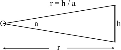
The geometrical relation captured by the fundamental stadimetric equation r = h/a.

In vision research one often uses “distance” instead of “range”. In this case distance is not used in its general (and conventional) sense, but in the sense of range as in gunnery, a directed distance from hither (the eye) to yonder (the object seen). In this paper we use both terms and treat them as synonymous, in the sense of “range”.

When the absolute size (as in the case of people) is not available, one may still use the size cue whenever multiple instances of some kind of object are simultaneously detected. Suppose one sees two instances of some type of object. Let these objects subtend angular sizes of a₁ and a₂, then the ratio of their two distances is d₁/d₂ = a₂/a₁. In this case the size cue yields ratios of distances.

Although distance ratios do not yield an absolute scale of distance, a set of distance ratios can often be calibrated easily, because even a single known distance suffices to fix the scale.

Depth and range (conventionally called “distance”) are categorically different entities. Distance is a non-negative quantity, with an obvious origin: distance zero is where the eye is. Thus the range, or distance domain, is the real half-line.

“Depth” is a subjective entity; it may have a variety of meanings. One such meaning is “estimated range”. In that case depth, like range, is a non-negative quantity with the eye at the origin. The case of pictorial space is categorically different. Pictorial depth has no obvious origin. The eye is not even in pictorial space; it is not at any particular depth at all. In fact, absolute depth is a non-entity. Only depth differences can be ascribed some meaning. Consequently, the depth domain is the full affine real line. The case of “visual space” is intricate. Here the meaning of “depth” varies according to the task, ranging from “estimated range” to “pictorial depth”.

There exists no causal or necessary functional relation between range and depth. In cases where ground truth exists (as in visual space) it is possible to establish an approximate, empirical functional relation. In cases of pictorial space this is not possible.

It is of some interest to design a speculative “ideal” depth-range function. Whether (and in which cases) such a function might approximately apply remains a matter of empirical research, of course.

Here is a heuristic reasoning:

Suppose one considers three locations A, B, and C in physical space, at corresponding ranges r_A, r_B, and r_C, say. Using the size cue, one might be able to measure the ratios r_Ar_B, r_B/r_C, and r_C/r_A. One has the trivial relation (r_A/r_B) × (r_B/r_C) = r_A/r_C.

Now suppose the distance ratios, r_A/r_B, r_B/r_C, and r_C/r_A would correspond to depth differences, d_AB, d_BC, and d_CA. What might the nature of such a relation be? Here are some constraints that appear “natural”:

• The depth difference of a location with itself should be zero; thus one requires that d_QQ = 0 for any location Q.

• The depth difference between two locations should change sign on the interchange of the locations; thus one requires that d_PQ = – d_QP for any locations P and Q.

• It is natural to assume the depth domain to be homogeneous (no “special” depth differences); thus the depth scale to be a linear scale. This implies the additivity of depths; thus one requires that d_PR = d_PQ + d_QR for any locations P, Q, and R. (This guarantees that depth is a “distance function” in the formal sense of mathematics. Of course, “distance” as used here is something else again!)

Together these three constraints imply that d_AB = log (r_A/r_B) = log r_A − log r_B. Apparently, the “natural” depth scale is an affine scale that may be understood as reflecting the logarithm of the range. Notice that this (formally) puts the eye at minus infinity—that is to say, the eye has no actual depth at all. We regard this as a natural consequence.

The logarithmic nature of the depth scale has an important implication. Consider some configuration viewed from a given vantage point. From the vantage point the elements of the configuration are seen in various directions. This is the configuration in the visual field, as a stellar configuration so to speak. In order to obtain a three-dimensional interpretation, one requires the range information. However, it is not necessary to specify the ranges of all points; it suffices to specify them only relatively, or by way of range ratios. The reason is that an arbitrary scaling (contraction or dilation) about the vantage point leaves the ratios of ranges invariant, whereas it affects the ranges themselves. In static, monocular vision (no binocular disparity, no movement parallax, no accommodation cue, and so forth) the absolute ranges are irrelevant; only their ratios are relevant. If the world suddenly grew ten times larger, you would never notice because this would not be optically specified. Lilliput is optically the same as Brobdignac, up to the moment Gulliver is introduced as an absolute unit of size (Swift 1726). If the ratios are invariant, then so are the depth differences. Thus the depths specify a configuration up to arbitrary scalings. They specify what is optically relevant, whereas the ranges contain information that is not properly optical.

This simple model may be naturally extended in the following way (Koenderink and van Doorn 2008). Consider the ground-plane of physical space, parameterized through the distance from the eyer and the azimuth a. Let the straight ahead be at azimuth a = 0, with azimuth increasing from left to right. Then any point may be specified by its Cartesian coordinates x, y = r (sin a, cos a), y in the straight ahead direction,x from left to right. The map (x, y) → (a, log r) is conformal, that is to say, is locally non-distorting (see Figure A2). It serves as a convenient model of the ground-plane in visual space.

Figure A2.

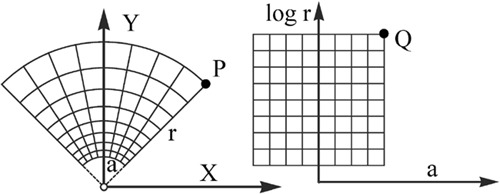
In the figure at left one has a Cartesian coordinate system (x, y), centered at the position of the eye. The range r and azimuth a of a point P (the upper right corner of the curvilinear pavement) have been indicated. At right the curvilinear pavement has been drawn after the conformal transformation discussed in the text. The point P maps on the point Q. This coordinate system has no natural origin. One may shift the transformed pavement freely along the log r axis. Notice that this map is indeed conformal in the sense that little squares in the ground-plane map on little squares of the image of the ground-plane in visual space.

In most cases of pictorial space the scale of the picture plane will not be calibrated; thus the azimuth is only known up to a (non-negative) factor. One has the map (x, y) → C (a, log = r) with C > 0. Then the depth coordinate would correspond to log r^C. This structure has been shown to explain the individual differences in the layout of pictorial relief in considerable quantitative detail (Koenderink et al 2001).

This two-dimensional model comes in handy if one needs to reason about the depth scale. In the model a unit increment in depth, that is, a range ratio of e¹ ≈ 2.72…, corresponds to a unit increment in azimuth, that is, one radian, or 57.3…deg. A fairly wide-angle view of 90 deg (that is π/2 radians), the extent of the “cone of vision” according to the classical authors, thus corresponds to a depth increment of also π/2 ≈ 1.57…, which implies a range ratio of e^π/2 ≈ 4.81….

The affine transformation d' = C (d + a), with C > 0, and a arbitrary, simply scales depth differences. That is to say, d₂′ − d₁′ = C (d₂ − d₁), irrespective the value of a. Thus the affine transformation scales all depth differences by the same factor. This transformation fully respects empirical depth difference data, since these can be obtained only up to a common factor. Apparently, the transformation conserves the relevant structure of depths; it leaves the depth domain invariant. This is the reason to say that the structure of the depth domain is the real number line modulo the group of affinities. This can be derived from first principles, departing from the observation that the optical structure available to a stationary vantage point in a static world is invariant with respect to arbitrary rotation-dilations about the vantage point (Koenderink and van Doorn 2008). It was empirically discovered by the German sculptor Adolf Hildebrand (1901), who described it in a book that became influential in art history of the early 20th century.

The relation derived via the heuristic is (of course) not necessarily a good description of the relation that one might find empirically. In this paper we are not able to test it, since we concentrated singularly on pictorial space, rather than visual space.

The logarithmic relation is formally the same as the relation proposed in the main text. This is not to say that it might be considered a “derivation”. The treatment in the main text is to be preferred, as it involves only a few very general arguments and does not depend upon any assumed relation to the geometry of physical space.

References

- Alberti L B. On Painting. New York: Penguin Classics; 1972. [Google Scholar]
- Balzer R. Peepshows: A visual history. New York: Harry N Abrams; 1998. [Google Scholar]
- Berkeley G. An essay towards a new theory of vision. Dublin, UK: Aaron Rhames; 1709. [Google Scholar]
- Brown J W. Self-embodying mind: Process, brain dynamics and the conscious present. Barrytown, NY: Barrytown/Station Hill Press; 2002. [Google Scholar]
- Chaldecott J A. “The zograscope or optical diagonal machine”. Annals of Science. 1953;9:315–322. doi: 10.1080/00033795300200243. [DOI] [Google Scholar]
- Comment B. The painted panorama. New York: Harry N Abrams; 1999. [Google Scholar]
- da Vinci L.1888The notebooks of Leonardo da Vinci—Complete (transl J P Richter)(13)http://www.g-utenberg.org/ebooks/5000
- Denis M. “Définition du néo-traditionisme”. Art et Critique. 1890;65 [Google Scholar]
- Emmert E. “Grössenverhältnisse der Nachbilder”. 1881. p. 19. Klinische Monatsblätter für Augenheilkunde.
- Fiske B A.1894. Method of and apparatus for range finding. Patent number 523 721
- Gibson J J. The perception of the visual world. Boston, MA: Houghton Mifflin; 1950. [Google Scholar]
- Gibson J J. “The information available in pictures”. Viewpoints. 1971;47:73–95. [Google Scholar]
- Gombrich E H. Art and Illusion. A study of the psychology of pictorial representation. London: Phaidon Press; 1960. [Google Scholar]
- Hildebrand A. Das Problem der Form in der bildenden Kunst. Strassburg, France: Heitz & Mündel; 1901. [Google Scholar]
- Kianush K. “A brief history of Persian Miniature”. Iran Chamber Society; 1998. http://www.irancham-ber.com/art/articles/history_iranian_miniature.php [Google Scholar]
- Koenderink J J, van Doorn A J. “The structure of visual spaces”. Journal of Mathematical Imaging and Vision. 2008;31:171–187. doi: 10.1007/s10851-008-0076-3. [DOI] [Google Scholar]
- Koenderink J J, van Doorn A J, Kappers A M L. “On so-called paradoxical monocular stereoscopy”. Perception. 1994;23:583–594. doi: 10.1068/p230583. [DOI] [PubMed] [Google Scholar]
- Koenderink J J, van Doorn A J, Kappers A M L, Todd J T. “Ambiguity and the ‘mental eye’ in pictorial relief”. Perception. 2001;30:431–448. doi: 10.1068/p3030. [DOI] [PubMed] [Google Scholar]
- Koenderink J J, van Doorn A J, Wagemans J. “Depth”. i-Perception. 2011;2:541–564. doi: 10.1068/i0438a-ap. [DOI] [PMC free article] [PubMed] [Google Scholar]
- Lane R. Images from the floating world: The Japanese print. New York: Putnam Publishing Group; 1978. [Google Scholar]
- Palmer S E. Vision science: Photons to phenomenology. Cambridge, MA: MIT Press; 1999. [Google Scholar]
- Penrose R, Todd J A. “On best approximate solution of linear matrix equations”. Mathematical Proceedings of the Cambridge Philosophical Society. 1956;52:17–19. doi: 10.1017/S0305004100030929. [DOI] [Google Scholar]
- Swift J.1726Gulliver's travels(Public domain: http://www.gutenberg.org/ebooks/829)
- van Doorn A J, Koenderink J J, Wagemans J. “Rank order scaling of pictorial depth”. i-Perception. 2011;2:724–744. doi: 10.1068/i0432aap. [DOI] [PMC free article] [PubMed] [Google Scholar]
- von Rohr M. “The Verant, a new instrument for viewing photographs from the correct standpoint”. The Photographic Journal. 1903;43:279–290. [Google Scholar]
- Wagemans J, van Doorn A J, Koenderink J J. “Measuring 3D point configurations in pictorial space”. i-Perception. 2011;2:77–111. doi: 10.1068/i0420. [DOI] [PMC free article] [PubMed] [Google Scholar]