

Abstract
This study explores the effects of various spatiotemporal dynamic texture characteristics on human emotions. The emotional experience of auditory (eg, music) and haptic repetitive patterns has been studied extensively. In contrast, the emotional experience of visual dynamic textures is still largely unknown, despite their natural ubiquity and increasing use in digital media. Participants watched a set of dynamic textures, representing either water or various different media, and self-reported their emotional experience. Motion complexity was found to have mildly relaxing and nondominant effects. In contrast, motion change complexity was found to be arousing and dominant. The speed of dynamics had arousing, dominant, and unpleasant effects. The amplitude of dynamics was also regarded as unpleasant. The regularity of the dynamics over the textures' area was found to be uninteresting, nondominant, mildly relaxing, and mildly pleasant. The spatial scale of the dynamics had an unpleasant, arousing, and dominant effect, which was larger for textures with diverse content than for water textures. For water textures, the effects of spatial contrast were arousing, dominant, interesting, and mildly unpleasant. None of these effects were observed for textures of diverse content. The current findings are relevant for the design and synthesis of affective multimedia content and for affective scene indexing and retrieval.
Keywords: emotion, dynamic textures, pleasure, arousal, dominance
1. Introduction
This study explores the effects of visual dynamic textures on human emotional experience. Dynamic textures are spatially repetitive, time-varying visual patterns that repeat or seem to repeat themselves over time. Dynamic textures extend the notion of self-similarity (central to conventional image texture) to the spatiotemporal domain. A dynamic texture may either be continuous or discrete. Discrete textures have clearly discernible parts (eg, a group of marching ants or fluttering leaves), whereas continuous textures represent media that are either continuous (eg, water or a waving flag that covers the entire field of view) or practically indiscernible thereof (eg, a waving field of grass seen from far away). Dynamic textures occur in nature and in videos of waves, moving clouds, smoke, fire, fluttering flags or foliage, traffic scenes, and moving masses of humans seen from a bird's eye view. Recently, dynamic textures have also appeared on large-scale digital billboards and electronic wallpaper (Huang and Waldvogel 2005). Dynamic textures are thus ubiquitous, and knowledge of their emotional effects may have important implications for the design and experience of our daily environment.
It has long been recognized that the emotional connotations of static visual textures are highly relevant for the appreciation of, for example, textile (Kim et al 2005), wall-paper, and surface coating (Wang 2009). As a result, the perceptual and emotional properties of static textures in general (eg, Machajdik and Hanbury 2010; Mao et al 2003), and the effects of their color distribution in particular (eg, Lucassen et al 2011; Simmons and Russell 2008), have been well documented. It appears that the human visual system is optimized for the perception of natural images (Field 1987, 1994; Parraga et al 2000), which typically have fractal-like spatiotemporal spectra (Billock 2000; Billock et al 2001a, 2001b). The amplitude spectra of dynamic natural textures closely follow an inverse power law relationship:
where fs and ft are, respectively, the spatial and temporal frequency, with 0.9 ≤ β ≤ 1.2 (M = 1.08; Billock 2000), and 0.61 ≤ α ≤ 1.2 (Billock et al 2001b). Spatial amplitude spectra approaching a f−1 distribution are typically considered pleasant, which is also reflected in EEG (Hagerhall et al 2008) and skin conductance (Taylor et al 2005) response. Deviations from a spatial f−1 distribution are perceived as unpleasant or uncomfortable (Fernandez and Wilkins 2008; Juricevic et al 2010; O'Hare and Hibbard 2011). White noise or 1/f0 is perceived as disorder, while f−2 is considered monotonous (Mao et al 2003). The functional visual brain circuitry that conveys the spatial frequency information is closely related and functionally linked to the circuitry that conveys emotional information (eg, Adolphs 2004; Amaral et al 2003). Emotional response to images may therefore indeed be modulated by their spatial frequency content (Delplanque et al 2007). Research on visual art indicates that complexity correlates positively with interest and has a non-linear relationship with pleasure (Forsythe et al 2011). Some of these findings have been used to develop algorithms that generate visual textures with a desired aesthetic perception, such as (non-)elegance and (dis-)like (eg, Groissboeck et al 2010).
The emotional experience of haptic (eg, Salminen et al 2011) and auditory (eg, Bigand et al 2005; Gomez and Danuser 2007) repetitive patterns has also been studied extensively. Music is well known to arouse strong emotional responses in people (Juslin and Västfjäll 2008). For instance, it is typically found that tempo is positively related to arousal (Bresin and Friberg 2000; Husain et al 2002) but mainly for popular music and in a non-linear manner (Kellaris and Kent 1993). Tempo is also positively related to happiness and negatively to sadness, while irregularity is negatively appraised and volume is generally positively related to arousal (Bresin and Friberg 2000).
In contrast, the emotional experience of visual dynamic textures is still largely unknown. Recently, dynamic textures have found applications in many different areas, such as animation (Chuang et al 2005), video classification (eg, Zhao and Pietikainen 2007), video retrieval (eg, Péteri and Chetverikov 2006; Smith et al 2002), and video synthesis (eg, Chan and Vasconcelos 2005; Constantini et al 2008; Doretto et al 2003; Lai and Wu 2007; Zhang and Wangbo 2007), and in the visualization of time-dependent vector fields (eg, Post et al 2003; Weiskopf et al 2003). The need to control their emotional effects is therefore increasing.
Visual imagery is one of the mechanisms through which auditory stimuli may induce emotion (Juslin and Västfjäll 2008). Musical characteristics such as repetition, melody, rhythm, and tempo are especially effective in stimulating vivid mental imagery (McKinney and Tims 1995). Music and visual information reciprocally influence emotion: music enhances the emotional experience of images (Baumgartner et al 2006), while visual stimuli in turn effectively modulate the structural and emotional experience of music (Boltz et al 2009). Visual imagery and music have a common temporal nature. It has been suggested that rhythm may be the link between the two (Chen et al 2011). It has indeed been shown that people “hear” purely visual rhythms (Guttman et al 2005), and that auditory signals drive perceived visual temporal rate (Recanzone 2003). Thus it seems that the brain attempts to create an emotional and structural congruent unified percept. Although music can be modeled by dynamic textures (Barrington et al 2010), it is unknown whether the emotional response to visual dynamic textures resembles the response to music with similar temporal characteristics.
In this study, observer experiments were performed to assess emotional experience as a function of the spatiotemporal characteristics of visual dynamic textures. Participants watched a set of dynamic textures, representing either water or a collection of various media, and self-reported their emotional experience.
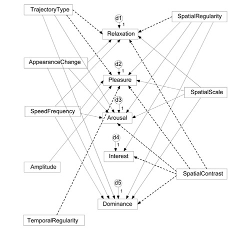
Based on knowledge about the emotional experience of auditory stimuli, it is hypothesized that (i) temporal regularity is positively related to pleasure, (ii) both the speed and amplitude of movement are positively related to arousal and negatively to relaxation, and (iii) complexity of motion and changes therein is positively related to interest. The hypothesized (baseline) structural model is graphically represented in Figure 1. Note that since this model is by nature exploratory, all spatiotemporal variables predict all emotional response variables.
Figure 1.
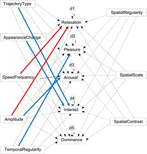
Hypothesized structural model describing the interrelations between temporal (left) and spatial (right) dynamic texture characteristics and human emotional response (middle). Blue (positive) and red (negative) colors indicate hypothetical path polarity (the sign of the correlation). d1–d5 represent residual disturbance terms.
2. General methods
2.1. Dynamic textures
Two stimulus sets were created from a total of 56 different dynamic textures that were manually selected from the DynTex database (Péteri et al 2010). Both sets had a high diversity of spatiotemporal characteristics. The first set consisted of 30 continuous dynamic textures representing only water (eg, sea, ponds, fountains, waterfalls, rivers; Figure 2). This collection will be called the “Water Set”.(1) The second set consisted of 36 textures representing both continuous and discrete textures of various semantic content (eg, crawling ants, fluttering leaves, rippling water, moving traffic, flickering candles; Figure 3). This collection will be called the “Mixed Set”.(2) Both sets had 9 water textures(3) in common.
Figure 2.
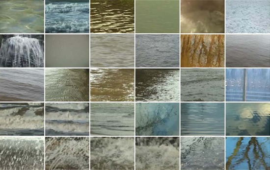
The Water Set, consisting of 30 different dynamic water textures from the DynTex database. See the animated version of this figure here.
Figure 3.
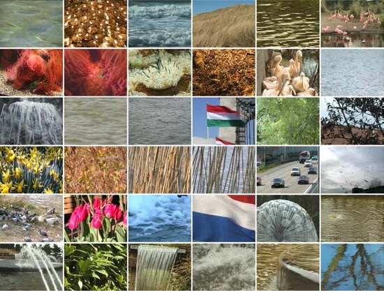
The Mixed Set, consisting of 36 different dynamic textures from the DynTex database. See the animated version of this figure here.
A set with elements representing a homogeneous medium from a single category (the Water Set) was used in an attempt to minimize potential confounding affective and cognitive effects of semantic image content. Also, the results obtained with this set may be related to earlier results that have been obtained for static water pictures (Nasar and Lin 2003).
In the classification phase of the experiments the textures were presented in their original format (720 × 576 pixels, 25 fps). In the rating phase the textures were displayed at 1/3 of their original size (240 × 192 pixels, 25 fps).
2.2. Spatio-temporal texture descriptors
The DynTex database also provides 10 structural descriptors for each dynamic texture, together with annotations that are based on a careful analysis of the underlying physical process that is represented (Péteri et al 2010).
The following five descriptors were used in the present study to quantify the temporal characteristics of the dynamic textures. TrajectoryType describes the complexity of motion and varies from still to straight to curving to oscillating to irregular, with values ranging from 1 to 5, respectively. AppearanceChange similarly describes the complexity of the change in the texture's appearance (eg, colour shifting) and varies from no change to directed to oscillating to irregular, with values 1 to 4, respectively. SpeedFrequency describes the speed of dynamics and varies from low to medium to high, with values ranging from 1 to 3, respectively. Amplitude describes the extent of the dynamics and varies from small to medium to large, with values ranging from 1 to 3, respectively. TemporalRegularity describes the regularity in terms of the former two variables over time and varies from low to medium to high, with values ranging from 1 to 3, respectively. Together, SpeedFrequency, TemporalRegularity, and AppearanceChange describe the temporal frequency content of a dynamic texture, while TrajectoryType and Amplitude relate to the optic flow in the stimulus pattern.
In addition, the following three descriptors were used to quantify the spatial characteristics of the dynamic textures. SpatialRegularity describes the amount of spatial variation in the dynamics (ie, the amount of different patterns occurring simultaneously) and varies from low to medium to high, with values 1 to 3, respectively. SpatialScale describes the scale of spatial variation between the moving parts of the texture and varies from fine to medium to coarse, with values ranging from 1 to 3, respectively. SpatialContrast analogously describes the extent of spatial variation between the moving parts of the texture and varies from low to medium to high, with values ranging from 1 to 3, respectively. Together, Spatial Regularity, Spatial Scale, and Spatial Contrast describe the spatial frequency content of a dynamic texture.
The temporal MainClass descriptor from the DynTex database was not used in this study, since it represents a rather subjective complex construct charactering the overall motion type. A fourth spatial descriptor called Density represents the discernability of the texture's individual parts and varies from sparse to medium to dense to continuous with values ranging from 1 to 4, respectively. In this study Density is only used in the analysis of the observer results for the Mixed Set, since this descriptor inherently applies only to textures showing discrete elements and not to continuous media.
2.3. Apparatus
Dell Precision 490 PC computers were used to present the dynamic textures to the observers and to register their response. The computers were equipped with Dell 19-inch monitors, with a screen resolution of 1280 × 1024 pixels, and a screen refresh rate of 60 Hz. Observers used standard mouse pointers to indicate their response and to move the dynamic textures on the screen.
2.4. Participants
It has previously been observed that the emotional experience of (static) textures is invariant for age, gender, personality and social class (Nasar and Lin 2003). Convenience sampling was therefore used to select the 107 participants of this study.
The experimental protocol was reviewed and approved by TNO internal review board on experiments with human participants and was in accordance with the Helsinki Declaration of 1975, as revised in 2000 (World Medical Association 2000). The participants gave their informed consent prior to testing. The participants received a modest financial compensation for their participation.
2.5. Analyis
SPSS 19 (www.spss.com) was used for the statistical analysis of the data. IBM SPSS AMOS 19 (Arbuckle 2010) was used evaluate the (hypothetical) baseline model shown in Figure 1 through covariance structure analysis.
Structural equation modeling (SEM) is a very general statistical modeling technique widely used in the behavioral sciences (eg, MacCallum and Austin 2000). SEM provides a very general and convenient framework for statistical analysis that includes several traditional multivariate procedures, such as factor analysis, path analysis, regression analysis, discriminant analysis, and canonical correlation as special cases. The basic idea differs from the usual statistical approach of modeling individual observations. In multiple regression or ANOVA the regression coefficients or parameters of the model are based on the minimization of the sum of squared differences between the predicted and observed dependent variables. SEM approaches the data from a different perspective. Instead of considering variables individually, the emphasis is on the covariance structure. Parameters are estimated in structural equation modeling by minimizing the difference between the observed covariances and those implied by a structural or path model. Among the strengths of SEM is the ability to construct latent variables: variables which are not measured directly, but are estimated in the model from several measured variables, each of which is predicted to ‘tap into’ the latent variables. This allows the modeler to explicitly capture the unreliability of measurement in the model, which in theory allows the structural relations between latent variables to be accurately estimated. Structural equation models are usually represented by a set of matrix equations and visualized by graphical path diagrams.
SEM allows both confirmatory and exploratory modeling; it is suited to both theory testing and theory development. Confirmatory modeling usually starts out with a hypothesis that gets represented in a causal model. The concepts used in the model must then be operationalized to allow testing of the relationships between the concepts in the model. The model is tested against the obtained measurement data to determine how well the model fits the data. The causal assumptions embedded in the model often have falsifiable implications, which can be tested against the data. With an initial theory, SEM can be used inductively by specifying a corresponding model and using data to estimate the values of free parameters. The initial hypothesis usually requires adjustment in light of model evidence.
We assessed the overall fit of the hypothesized model to the data using several goodness-of-fit measures, such as the χ2 goodness-of-fit test; the Comparative Fit Index (CFI; Bentler 1990); the model residual, measured by the Root Mean Square Error of Approximation (RMSEA; Steiger 1990); and relative goodness of fit, measured by the Akaike Information Criterion (AIC; Akaike 1974, 1987). A significant χ2 statistic may suggest that the hypothesized model does not adequately fit the observed data, whereas a non-significant χ2 suggests model adequacy. However, this index is sensitive to sample size and violations of the assumption of multivariate normality. Therefore, alternative fit indices are generally used (Schermelleh-Engel et al 2003). The CFI indexes the relative change in model fit as estimated by the noncentral chi-square of a target model versus the independence model. The RMSEA measures the discrepancy due to approximation and is relatively independent of sample size. The AIC adjusts χ2 for the number of estimated parameters.
3. Experiment I: Affective dynamic texture descriptors
A preliminary experiment was performed to select the most appropriate adjectives describing the affective properties of dynamic textures. The widely used and well-validated Pleasure-Arousal-Dominance (PAD) emotional state model (eg, Arifin and Cheung 2007; Mehrabian 1996) was used in this study to encode the affective characteristics of the dynamic textures. This model states that the emotional spectrum can reliably be described along three bipolar dimensions: pleasure-displeasure (ie, affect), relaxed/aroused (ie, intensity), and controlling/controlled (ie, dominance). The participants' emotional response to their viewing of the dynamic textures was measured by self-report through the use of a scoring list of affective adjectives. Self-report has been shown to be a reliable measure of emotional reactions to audio-video clips and is consistent with five peripheral physiological signals: galvanic skin resistance (GSR), electromyograms (EMG), blood pressure, respiration patterns, and skin temperature (Soleymani et al 2008).
3.1. Methods
3.1.1. Affective terms.
A list of 58 candidate affective adjectives was compiled from a literature study (eg, Cerf et al 2007; Fujiwara et al 2006; Küller 1975; Masakura et al 2006; Russell 1980; Russell et al 1981; Russell and Pratt 1980; see Figure 4). These 58 candidate adjectives were first divided into 10 categories. Eight categories corresponded to the ends of the four axes of Russell's circumplex model of affect (Pleasure, Arousal, Interest, Relaxation [Russell 1980]; see upper section of Figure 4). The remaining two categories corresponded to the ends of the Dominance scale (Figure 4 lower section). Then, a scoring list was made which listed all 58 candidate terms in a spatial layout that grouped the 52 adjectives in the Pleasure, Arousal, Interest, and Relaxation categories according to a circumplex ordering (Figure 4 upper section) and listed the 6 adjectives in the Dominance category in a separate section (Figure 4 lower section). The circumplex ordering was achieved by mapping the eight categories from Russel's model onto the eight outer cells of a 3 × 3 square matrix (see also the left button section of Figure 6).
Figure 4.
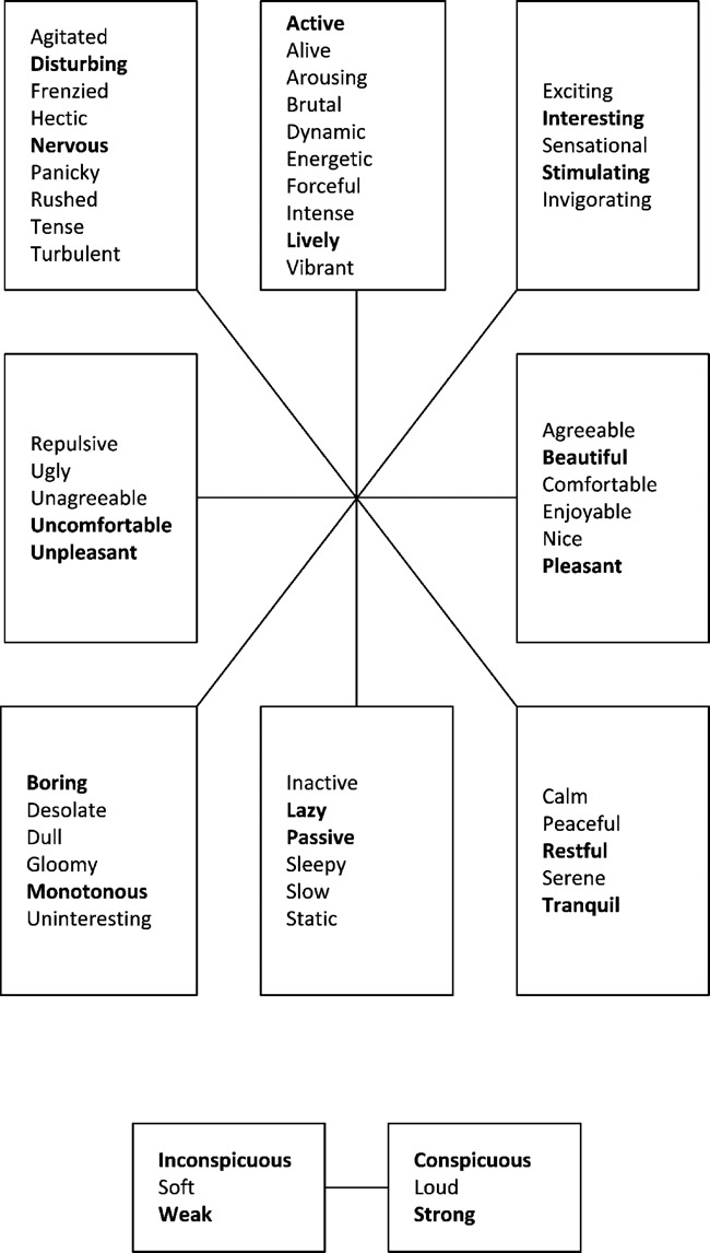
Upper 3 rows: Eight categories of candidate affective adjectives ordered corresponding to Russell's circumplex model of affect (Pleasure – middle row, Arousal – middle column, Interest – lower-left to top-right diagonal, Relaxation - top-left to lower right diagonal [Russell 1980]; see also Figure 5). Lower row: Two categories corresponding to the Dominance scale (left: non-dominant; right: dominant). The two most frequently selected adjectives in each category are printed in bold.
Figure 6.
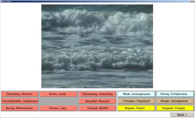
Screen layout during the affective classification phase of the experiment. The dynamic texture is shown on top. Buttons in the left section correspond to the Pleasure-Arousal scale. Buttons in the right section correspond to, respectively, Dominance (weak, inconspicuous - strong, conspicuous), SpatialStructure (complex, organized - simple, disorganized), and TemporalStructure (regular, fluent - irregular, choppy).
Figure 5.
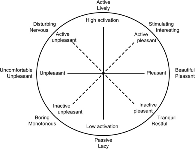
A two-dimensional representation of the self-report affect circumplex space, with 8 circularly ordered affective states represented by two adjectives each (after Russell 1980). The horizontal axis corresponds to Pleasure, the vertical axis to Arousal, the right-diagonal to Interest, and the left-diagonal to Relaxation.
3.1.2. Participants.
A total of 24 participants (14 males and 10 females), ranging in age from 18 to 55 years (M = 36.2, SD = 15.9) participated in this experiment.
3.1.3. Stimuli.
The stimuli were 36 highly diverse (with respect to spatial and temporal characteristics, and with respect to semantic scene content) dynamic textures from the DynTex database.(4)
3.1.4. Procedure.
Before starting the experiment the participants read the experimental instructions. These instructions explained that the participants should attribute the most appropriate adjectives from a given list of candidate affective adjectives to each of presented dynamic textures. The participants were informed about the nature of Russell's circumplex model of affect (Russell 1980), and in particular about the fact that affective terms close to each other on the perimeter of the circumplex refer to similar emotions while terms on opposite sides of the same bipolar axis are mutually exclusive. The participants were asked to select at least one term from the entire set of 8 categories representing the circumplex model of affect. They were allowed to select more than one term, and terms in adjacent (in the circumplex model) categories, with a maximum of three terms from a single category. Additionally, they were asked to select at least one term from each of the two dominance categories. It was emphasized that the participants should ignore the semantic content of the video clips and base their judgments solely on the spatiotemporal characteristics of the textures, preferably using their first impression. Each participant privately watched the entire stimulus set and performed the experiment self-paced without any time restrictions. The experiment typically lasted about an hour.
3.2. Results
Four adjectives had item-total correlations smaller than 0.3 or reduced Cronbach's alpha inter-item reliability score in the category below 0.7 and were therefore deleted for lack of reliability. Finally, the two most frequently scored adjectives in each category were selected (see bold printed adjectives in Figure 4), and categories on opposite ends of the circumplex model were joined. The result was a list of 28 appropriate affective terms. The resulting dimensions were Relaxation (disturbing, nervous – tranquil, restful), Pleasure (uncomfortable, unpleasant – beautiful, pleasant), Arousal (passive, lazy – active, lively), Interest (boring, monotonous – stimulating, interesting), and Dominance (weak, inconspicuous – strong, conspicuous). These five dimensions were used to measure emotional response in the rest of this study. The two additional dimensions Complexity (complex, organized – simple, disorganized) and Regularity (regular, fluent – irregular, choppy) were adopted to measure the participants' impression of, respectively, the spatial and temporal textures characteristics (see Figure 6).
4. Experiment II: Affective rating of dynamic textures
A second experiment was performed to measure the degree to which the affective classifiers determined in Experiment I applied to each of the dynamic textures of the Water Set and the Mixed Set. In addition, the spatiotemporal characteristics of the dynamic textures were investigated through the concepts of spatial complexity and temporal regularity.
4.1. Participants
The set of dynamic water textures was judged by 38 participants (22 males and 16 females), whose age ranged from 19 to 64 years (M = 37.0, SD = 16.2). The set of mixed dynamic textures was judged by 45 participants (23 males and 22 females), ranging in age from 18 to 64 years (M = 34.8, SD = 17.5).
4.2. Procedure
Before starting the experiment the participants read the experimental instructions. These instructions explained the experimental procedure, the stimulus presentation programme, and its response buttons, and showed screen shots from all stages of the experiment. The instructions emphasised that the participants should ignore the semantic content of the dynamic textures and should base their judgments solely on their spatiotemporal characteristics, preferably using their first impression. The participants were also informed about the nature of Russell's circumplex model of affect (Russell 1980), and in particular about the fact that affective terms close to each other on the perimeter of the circumplex refer to similar emotions, while terms on opposite sides of the same bipolar axis are mutually exclusive. The participants were asked to select at least one and most two (adjacent) affective terms from the left response button section and to select exactly one term on each of the 3 rows on the right response button section. The participants could indicate their selection by placing the cursor successively over the corresponding response buttons on the screen and clicking a mouse button (see Video 1).
An experimental run consisted of two parts. In the first part of the experiment the participants attributed each dynamic texture the appropriate affective and spatiotemporal classification terms. In the second part of the experiment, the participants rank ordered the dynamic textures according to the classification terms that had been attributed in the first part of the experiment.
A typical run went as follows. After the participants had read the instructions, the experimenter selected the appropriate set of dynamic textures (ie, either the water or the mixed set) and started the test programme in the texture classification mode. The test programme then presented the first dynamic texture of the test set in the upper half of the screen, while the lower half of the screen showed two sections with response buttons (Figure 6). The buttons in the left section correspond to categories from Russell's circumplex model of affect (Pleasure and Arousal; Russell 1980). The buttons in the right response section correspond, respectively, to Dominance (weak, inconspicuous - strong, conspicuous), spatial Complexity (complex, organized - simple, disorganized), and temporal Regularity (regular, fluent - irregular, choppy). The participants then classified the texture by pressing the buttons labelled with the affective and structural terms that corresponded most closely to their impression of the texture. A button changed colour when activated. A previous classification could be undone by pressing an activated button a second time. When they were satisfied with their classification, the participants could press a button labelled “Next” to proceed to the next dynamic texture. When all textures in the test set had been labelled the test programme displayed a message that the rating phase would start when the “Next” button was pressed again. In the rating mode, the participants successively rank ordered the dynamic textures with respect to each of the classification terms that they had previously attributed to the textures during the first part of the experiment. Because of this procedure, a different number of dynamic textures (ranging from 0 to the cardinality of the test set) may correspond to (and therefore need to be rated for) a given classification term. This procedure was chosen to restrict the experimental time (rating all textures with respect to all classification terms takes a large amount of time, and may easily lead to observer fatigue), and to keep the participants motivated (rating many textures with respect to terms that obviously don't apply may easily induce boredom).
In the rating mode, all dynamic textures in a given category (ie, textures to which a given classification term had been attributed) were initially shown in the upper part of the screen (Figure 7a). A scale bar in the middle of the screen showed the current classification term together with the range of the scale (ie, the degree to which the classification term applies to the dynamic texture: ranging from 0 = “not at all” to 1 = “very much”). A participant could then drag the dynamic textures from the upper part of the screen to the lower part using a mouse (Figure 7b). The horizontal position of the midpoint of a dynamic texture patch is adopted as its value on the rating scale. When all dynamic textures in a category had been ordered with respect to their common classifier, the participant could proceed to the next texture category by pressing a button that appeared in the upper part of the screen (Figure 7c). Before this button was pressed, the order of the dynamic textures could still be adjusted.
Figure 7.
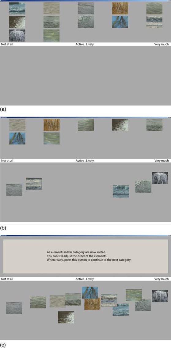
Screen layout during the affective rating phase of the experiment. This example illustrates the rating of dynamic water textures. (a) Initially, all dynamic textures in a given category are shown in the upper part of the screen. A scale bar in the middle of the screen shows the classification term (in this example: Active, Lively) and the range of the scale (ie, the degree to which the classification term applies to the dynamic textures: ranging from 0 = “not at all” to 1 = “very much”). (b) Participants can drag the dynamic textures from the upper part of the screen to the lower part using a mouse. The horizontal position of the midpoint of a dynamic texture patch is adopted as its value on the rating scale. (c) When all dynamic textures in a category have been ordered with respect to their common classifier, the participant can proceed to the next texture category by pressing a button that appears in the upper part of the screen. Before pressing this button, the order of the dynamic textures can still be adjusted.
The test programme allowed the simultaneous presentation of an arbitrary number of video clips on a regular computer. Hence, all textures could dynamically be presented simultaneously at their full frame rate. If there were more textures in a category than could simultaneously be represented in the upper display area, the programme initially showed only the first elements of the category. Each time a texture was moved to the lower part of the screen, a new element from the category appeared in the display area that had become available in upper part of the screen, until finally all textures in the category were represented on the screen.
The experiments were performed self-paced without any time restrictions. A single run typically lasted between 30 and 45 minutes.
4.3. Preliminary analyses
The mean rating scores were computed for each texture in both (Water and Mixed) datasets and for all classification terms. The two resulting datasets with scores on the spatiotemporal characteristics (Table 1) and mean scores for the emotional response variables for each texture (Table 2) were then used as groups in the model of Figure 1, which was trimmed and then analysed for multi-group invariance.
Table 1. Descriptive statistics (Mean and Standard Deviation) of the spatiotemporal characteristics of the Water and Mixed stimulus sets. See text for an explanation of the descriptors.
| Descriptor | Water textures |
Mixed textures |
||
| M | SD | M | SD | |
| Trajectory type | 3.733 | 1.081 | 3.597 | 1.189 |
| Appearance change | 3.400 | 1.020 | 2.778 | 1.180 |
| Speed frequency | 2.333 | 0.547 | 2.250 | 0.500 |
| Amplitude | 1.300 | 0.837 | 1.500 | 0.878 |
| Temporal regularity | 1.733 | 0.450 | 1.861 | 0.351 |
| Spatial regularity | 1.667 | 0.606 | 1.694 | 0.467 |
| Spatial scale | 1.767 | 0.504 | 1.778 | 0.540 |
| Spatial contrast | 1.500 | 0.509 | 1.722 | 0.513 |
Table 2. Descriptive statistics (Mean and Standard Deviation) of the emotional (Relaxation, Pleasure, Arousal, Interest, Dominance), spatial (Complexity), and temporal (Regularity) response variables of the Water and Mixed stimulus sets. See text for an explanation of the descriptors.
| Response variable | Water textures |
Mixed textures |
||
| Mean | SD | Mean | SD | |
| Relaxation | 0.551 | 0.242 | 0.560 | 0.177 |
| Pleasure | 0.548 | 0.222 | 0.536 | 0.184 |
| Arousal | 0.479 | 0.249 | 0.454 | 0.211 |
| Interest | 0.460 | 0.209 | 0.451 | 0.156 |
| Dominance | 0.480 | 0.239 | 0.496 | 0.154 |
| Complexity | 0.479 | 0.249 | 0.448 | 0.178 |
| Regularity | 0.522 | 0.233 | 0.538 | 0.186 |
Absolute values of the multivariate kurtosis and all the endogenous variables' skew and kurtosis values were less than 3, and none of the endogenous variables had p-values smaller than .05 for the Kolmogorov-Smirnov and Shapiro-Wilk normality tests. Linearity was found roughly between only certain variables, but for these cases no curvilinear relationships were found either. Box-plots and Mahalanobis distances revealed no significant outliers. No other assumptions were violated. All statistical model assumptions were thus found to hold.
The response variables Complexity and Regularity are directly related to the spatiotemporal stimulus descriptors from the DynTex database: Regularity represents an overall impression of TrajectoryType, SpatialRegularity, TemporalRegularity, and AppearanceChange, while Complexity refers to an overall impression of SpatialContrast, Amplitude, SpeedFrequency, and SpatialScale. Hence, it is of interest to know to what extent these descriptors indeed explain the participants' impressions of the dynamic textures. A regression analysis was therefore performed with Complexity as the dependent variable and the spatio-temporal texture descriptors as the independent variables. R2 was 0.576. When the analysis was performed with Regularity as the dependent variable, R2 was 0.596. Hence, the spatio-temporal descriptors indeed adequately explain the participants' impressions of the textures.
4.4. Model modification
Firstly, all regression paths in the initial model from Figure 1 that were not significant for both (water and mixed) data sets were deleted one by one, starting with the paths with the highest p-values and working down. All regression paths were then one by one constrained to be equal across the data sets, starting with the paths that had the greatest inter-set differences in regression coefficients and p-values. Constraints were kept only if they did not significantly degrade the model fit (ie, if they resulted in an insignificant increase in χ2). Since the two datasets result from two different observer populations watching different dynamic texture sets, the resulting path constraints indicate that the corresponding relationships are invariant across populations and texture types, and consequently have high internal and external validity and high replicability. The comparative model fit over the independence model, measured by the Comparative Fit Index (CFI), the model residual, measured by the Root Mean Square Error of Approximation (RMSEA), and the relative goodness of fit, measured by the Akaike Information Criterion (AIC), are all better for the final than for the unconstrained model, and changes in these statistics were generally in line with changes in χ2. After adding the valid constraints, no p-values exceeded 0.25, so the model was not further trimmed. The final model is presented in Figure 8.
Figure 8.
The final model. Dashed lines represent relationships that vary per texture set.
4.5. Final results
Table 3 reports the regression path coefficients of the final model shown in Figure 8 (the coefficients are not included in this figure to prevent clutter). For the standardised regression coefficients, values below 0.3 can be considered as weak, values between 0.3 and 0.5 as modest, and values larger than 0.5 as strong.
Table 3.
Regression coefficients for the paths in the final structural equation model. For estimates that are different for the two (water and mixed) stimulus sets, the values are reported as [estimate water set]/[estimate mixed set].

TrajectoryType was a modest, positive predictor of Relaxation for the water textures: water in complex motion was perceived as relaxing. However, this relation may be specific for homogeneous or water textures, since no such relation was observed for dynamic textures with diverse content. There was a trend towards significance for a relation between TrajectoryType and Pleasure. This relation was positive for water textures, but negative for textures of diverse content, providing tentative support that (like in visual art) the relation between pleasure and complexity is non-linear. Linearity tests correspondingly found only very rough linearity. TrajectoryType had a weak, negative correlation with Arousal and Dominance for both stimulus sets, indicating that arousal and dominance both increase with motion complexity. In sum, motion complexity generally has a slightly relaxing and weakening effect on the perception of a dynamic texture, while its effect on pleasure may be non-linear.
AppearanceChange correlated positively with Arousal and Dominance and negatively with Relaxation. The effects were all weak for the Water Set and modest for the Mixed Set. All relations were invariant between the two texture sets and thus had high validity. In contrast with the complexity of motion itself, the complexity of changes in the motion of a texture is thus perceived as dominant and arousing.
SpeedFrequency correlated modestly and positively with Dominance and Arousal, and it correlated weakly and negatively with Relaxation and Pleasure. All relations were invariant between the two texture sets. As such, the speed of a texture's dynamics has a dominant and arousing effect that is regarded as unpleasant. Amplitude only predicted Pleasure, and the correlation was negative and invariant between the two texture sets: it was modest for the Water Set and weak for the Mixed Set. That is, the extent of a texture's dynamics has an unpleasant effect. TemporalRegularity, which describes the regularity of the previous two variables, had a modestly positive correlation with Pleasure for the Water Set, but no relation for the Mixed Set. The desirability of dynamic regularity in textures may thus be content specific.
SpatialRegularity correlated weakly positively with Relaxation. Correspondingly, there was a weak and negative correlation with Arousal. SpatialRegularity also correlated weakly positively with Pleasure. Its relation with Dominance was modestly negative, and the relation with Interest was weakly negative. All relations were invariant between the two texture sets, except the relation with Relaxation, and that relation also did not vary in strength. In conclusion, a texture with more regularity in space, or less different dynamics occurring simultaneously, elicits somewhat more relaxation and pleasure and less interest, and is perceived as less dominant.
SpatialScale correlated negatively with Relaxation and positively with Arousal. All effects were weak, except the negative correlation with Relaxation for the Mixed Set, which was modest. SpatialScale also correlated weakly positively with Dominance. Its relation with Pleasure was modestly negative for the Water Set and strongly negative for the Mixed Set. All relations were invariant between the two texture sets. Similar to the speed of a texture's dynamics, the relative surface area of the dynamics has an unpleasant, arousing, and dominant effect, which is greater for the Mixed Set than for the Water Set.
SpatialContrast had no relations with the emotional response variables for the Mixed Set. For the Water Set, it correlated modestly positively with Arousal and a modestly negatively with Relaxation. SpatialContrast furthermore correlated weakly negatively with Pleasure and modestly positively with both Interest and Dominance. In conclusion, the effects of a water texture's degree of spatial variation are arousing, dominant, mildly unpleasant, and interesting. These effects are not seen for textures of diverse content.
Table 4 presents the proportions of explained variance for the dependent variables. In line with the many significant predictors, explained variance was around 50% for all variables except Pleasure for the water textures and Interest in general. Proportions around 50% are typically considered a significant amount for indeterminate concepts like emotions (Kline 2010, p. 185; denotes values below 1% as small, 10% as typical or medium, and values above 30% as large). These results also indicate that the selected spatio-temporal video characteristics adequately characterise a dynamic texture with regard to its effects on emotional response. Even the values for Interest are more in the range of “typical” than “small”. Table 5 reports the variances of all the predictors and the residual error terms. All variances were significant. This finding indicates that there was significant variability in the spatio-temporal characteristics of the selected dynamic textures. Note that, in agreement with the high proportions of explained variance, the variances of the residual error terms are small relative to those of the predictors.
Table 4. Proportions of explained variance (R2) for the dependent variables.
| Pleasure | Arousal | Dominance | Interest | Relaxation | |
| Water set | 0.734 | 0.554 | 0.475 | 0.150 | 0.560 |
| Mixed set | 0.571 | 0.492 | 0.530 | 0.042 | 0.496 |
Table 5. Variances of the predictor variables.
| Predictor | Water set |
Mixed set |
||||
| σ2 | S.E. | p | σ2 | S.E. | p | |
| Trajectory type | 1.129 | 0.296 | <0.001 | 1.372 | 0.329 | <0.001 |
| Appearance change | 1.007 | 0.264 | <0.001 | 1.353 | 0.324 | <0.001 |
| Speed frequency | 0.289 | 0.076 | <0.001 | 0.243 | 0.058 | <0.001 |
| Amplitude | 0.677 | 0.177 | <0.001 | 0.750 | 0.180 | <0.001 |
| Temporal regularity | 0.196 | 0.051 | <0.001 | 0.120 | 0.029 | <0.001 |
| Spatial regularity | 0.356 | 0.093 | <0.001 | 0.212 | 0.051 | <0.001 |
| Spatial scale | 0.246 | 0.064 | <0.001 | 0.284 | 0.068 | <0.001 |
| Spatial contrast | 0.250 | 0.066 | <0.001 | 0.256 | 0.061 | <0.001 |
| d1 (relaxation) | 0.029 | 0.008 | <0.001 | 0.016 | 0.004 | <0.001 |
| d2 (pleasure) | 0.019 | 0.005 | <0.001 | 0.017 | 0.004 | <0.001 |
| d3 (arousal) | 0.029 | 0.008 | <0.001 | 0.021 | 0.005 | <0.001 |
| d4 (interest) | 0.037 | 0.010 | <0.001 | 0.021 | 0.005 | <0.001 |
| d5(dominance) | 0.025 | 0.007 | <0.001 | 0.013 | 0.003 | <0.001 |
5. Discussion
The relation between various spatiotemporal characteristics and emotional experience was studied for visual dynamic textures. Motion complexity was found to have mildly relaxing and nondominant effects. In contrast, motion change complexity was found to be arousing and dominant. The speed of dynamics had arousing, dominant and unpleasant effects. The amplitude of dynamics was also regarded as unpleasant. The regularity of the dynamics may interact with video content in eliciting emotions. The regularity of the dynamics over the textures' space was found to be uninteresting, nondominant, mildly relaxing, and mildly pleasant. The spatial scale of the dynamics had an unpleasant, arousing, and dominant effect, which was larger for textures with diverse content than for water textures. For water textures, the effects of spatial contrast were arousing, dominant, interesting, and mildly unpleasant, but none of these effects were found for textures of diverse content.
These results only partially agree with the hypotheses, which demonstrate that the effects are domain specific and the hypotheses cannot easily be derived from literature on other sensory domains, such as the studies on the emotional response to auditory or tactile stimuli. Hypothesis (i)—temporal regularity is positively related to pleasure—was only supported for the set of water textures: no relation was found for the set of mixed textures. Hypothesis (ii)—both the speed and amplitude of movement are positively related to arousal and negatively to relaxation—was supported for the speed of the dynamics, but not for their amplitude. Amplitude did not significantly correlate with either Arousal or Relaxation. Finally, hypothesis (iii)—complexity of motion and change therein is positively related to interest—was not even partially supported. Neither motion complexity nor motion change complexity correlated significantly with Interest.
The present study shows that the speed of a texture's dynamics has a dominant and arousing effect. This finding agrees with the result of an earlier study on static imagery of water textures where it was found that stillness is perceived as relaxing and that (the impression of) movement is perceived as exciting (Nasar and Lin 2003). The current finding that complexity correlates positively with pleasure for water textures agrees with the earlier results that composite water textures are preferred over simple ones (Nasar and Lin 2003), and that complexity correlates positively with interest in visual art (Forsythe et al 2011). The present result that complexity, speed, and amplitude of movement all serve to increase arousal also agrees with similar findings from the tactile domain, where it was found that “Smooth” stimuli elicit a lethargic feeling, and “Prickly” elicits a nervous feeling, while an increase in frequency and amplitude is positively correlated with the intensity of the emotional response (Suk et al 2009).
Certain findings are of particular interest. AppearanceChange correlated positively with Arousal and Dominance and negatively with Relaxation, and these relations were all weak for the water textures but moderate for the textures of diverse content. This discrepancy in strength may have occurred because water textures all have relatively high and invariant motion change complexity (Mwater = 3.400, SDwater = 1.020; Mmixed = 2.778, SDmixed = 1.180), so that participants watching the Water Set may have adapted to its effects while participants watching the Mixed Set had less opportunity to adapt.
The effects of SpatialContrast also differed greatly between the two texture sets. SpatialContrast correlated significantly with several emotional response variables for the Water Set, but it was not a significant predictor for any variable in the Mixed Set. It is hypothesised that this distinction occurs because the spatial contrast of the diverse textures exists predominantly between different objects (eg, cars, flora), for which different dynamics are naturally expected. Conversely, the spatial variation of water textures occurs within the same homogeneous water mass and may in consequence be perceived as more unexpected and chaotic. To informally test this hypothesis, a regression analysis was performed with SpatialContrast∗Density as the predictor of the emotional response variables. Density is additional annotation in the DynTex database and describes the discernability of a texture's individual parts and varies from sparse to medium to dense to continuous, with values ranging from 1 to 4, respectively. A significant interaction between Densityand SpatialContrast was found for Relaxation (p = 0.046; β = 0.334) and Arousal (p = 0.023; β = 0.378), providing tentative support for the hypothesis.
Interest was an outlier with regards to the relatively low amount of its variance that could be explained by the spatiotemporal texture characteristics. It is hypothesised that interest is primarily determined by content, although spatio-temporal texture characteristics evidently play a significant role as well.
The current rating procedure was adopted because it was observed in earlier experiments that participants tend to forget their responses for similar samples shown earlier in a trial when samples are shown individually one after the other (Lucassen et al 2011). This would increase the response variability and reduce intra- and inter-observer correlations. A possible limitation of the present emotional response rating procedure is that it may be prone to bias. In this study, the participants assigned the stimuli to several emotional classes during a first viewing and ranked all stimuli in each class during a second viewing. Hence, habituation (both by repeated viewing of the same stimuli and by simultaneously viewing all stimuli in the same class) may have diminished the emotional response during the second viewing of the textures, which would imply that the results underestimate the true effects. A procedure in which the stimuli are rated individually may be less prone to this type of bias. Also, presenting each texture individually instead of the simultaneous presentation of all previously selected textures eliminates relativity biases. In this study, the participants (despite their instructions) may merely have rated the textures relative to the other textures that were simultaneously presented, instead of using the absolute scale of 0 to 1. Fortunately, no statistical problems were observed as a result of the chosen methodology, and all indicators of the study's validity were favourable. As most of the relations were invariant across the two stimulus sets (ie, for different textures and participants), the results (though exploratory) had high internal and external validity. The selected spatio-temporal characteristics furthermore explain large amounts of the emotional response variance and thus adequately characterise the dynamical textures. After standardisation, the observed relations were stronger for the mixed textures than for the set of water textures. This suggests that the current findings may even underestimate the emotional effects of dynamic textures in real life. In addition, the current results may also underestimate these effects because of the small angular size of the stimuli that were used (about 18 deg). In real life dynamic textures may fill a much larger part of the visual field of the observer, which may significantly enhance the effects that were observed here (eg, Lin et al 2007).
Taking into account the high prevalence of dynamic textures in nature and their increasing importance in digital media, the current findings may have important practical implications for designers and observers of dynamic sceneries. Possible applications are the synthesis of affective multimedia content (eg, backgrounds for games, video clips, or digital wallpaper; eg, Houtkamp et al 2008), the design of restorative or healing environments (Dijkstra et al 2006), and affective video retrieval (Hanjalic 2006, Hanjalic and Xu 2005). For instance, virtual environments can be made emotionally more compelling by introducing dominant and arousing dynamic textures, such as large and fast breaking waves, that heighten tension and create dramatic effects (Houtkamp et al 2008). Similarly, the restorative value of healing environments may benefit from the introduction of relaxing dynamic textures like slowly undulating water surfaces or waving corn fields (Dijkstra et al 2006). Displays on empty train stations may stimulate the lonely or bored traveller by showing interesting and complex dynamic patterns, while the same displays may have a relaxing effect on hurried and aroused travellers by showing simple and slow moving patterns when stations are crowded and tension mounts (Van Hagen 2011). Most spatiotemporal dynamic texture descriptors from the DynTex database have a direct relation with computer vision algorithms (Péteri et al 2010). The relation between these descriptors and human emotional experience therefore enables the automatic indexing and retrieval of affective video content.
Future research could investigate the hypothesised explanations for some of the current findings, such as a non-linear relationship between complexity and pleasure, that spatial contrast evokes emotional responses only if it occurs within the same object and that interest is predominantly a result of content. Interaction effects between the relationships that were observed in this study could also be explored. It would also be interesting to compare the results for the Water Set with those obtained for other continuous or semi-continuous media (eg, waving textile or grass), to investigate whether the difference between the results for the Water Set and the Mixed Set reflects a semantic component or the fact that not all observer impressions are captured by the current set of descriptors. Finally, it could be tested if the results of this study can be extrapolated to non-recurrent textures, which would be of significance for the emotional experience of people's entire visual surroundings.
Acknowledgments
This research was supported by NWO-VICI grant 639.023.705 Color in Computer Vision.
Biography
 Alexander Toet received his PhD in physics from the University of Utrecht, Utrecht, The Netherlands in 1987, where he worked on visual spatial localization (hyperacuity) and image processing. His is currently a guest researcher at the Intelligent System Laboratory Amsterdam, Faculty of Science, University of Amsterdam, where he investigates the effects of color on affective image classification, and a senior research scientist at TNO (Soesterberg, The Netherlands), where he investigates multimodal image fusion, image quality, computational models of human visual search and detection, and the quantification of visual target distinctness. He also studies crossmodal perceptual interactions between the visual, auditory, olfactory, and tactile senses, with the aim to deploy these interactions to enhance the affective quality of virtual environments for training and simulation.
 Menno Henselmans received his BSc (Social Sciences with a minor in statistics) with magna cum laude at the University College Utrecht, The Netherlands in 2011. He is currently a Behavioral and Economic Science Master student at the University of Warwick, UK.
 Marcel Lucassen received his MSc degree in technical physics from Twente University and his PhD in biophysics (on color constancy) from Utrecht University, The Netherlands. Thereafter he worked with Akzo Nobel Coatings and TNO Human Factors in research and management positions. He is now a freelance color scientist at Lucassen Colour Research and holds a part-time position at the University of Amsterdam. His research interests are in basic and applied color vision.
 Theo Gevers is an Associate Professor of Computer Science at the University of Amsterdam, The Netherlands, where he is also teaching director of the MSc of Artificial Intelligence. He is a full professor at the Computer Vision Center of the Universitat Autonoma de Barcelona, Spain. He currently holds a VICI award (for excellent researchers) from the Dutch Organisation for Scientific Research. His main research interests are in the fundamentals of color image processing, image understanding, and computer vision. He is chair of various conferences, and he is associate editor for the IEEE Transactions on Image Processing. Further, he is program committee member of a number of conferences, and an invited speaker at major conferences. He is a lecturer of post-doctoral courses given at various major conferences (CVPR, ICPR, SPIE, CGIV).
Footnotes
The 30 dynamic textures in the Water Set had the following identifiers in the DynTex database: 6ame100, 54ab110, 54pf110, 54pg110, 55fa110, 64adf10, 64adl10, 64cb810, 571b110, 571b310, 644c610, 647b110, 647b210, 647b410, 647b710, 647b810, 647c310, 648e510, 649dd10, 649de10, 649h310, 649i410, 649i810, 649ic10, 6484f10, 6484i10, 6485110, 6485210, 6487510, 6489510.
The 36 dynamic textures in the Mixed Set had the following identifiers in the DynTex database: 6ame100, 6ammi00, 54ab110, 54ac110, 54pf110, 64aa410, 64ab410, 64ab510, 64ad410, 64ad910, 64adb10, 64adf10, 64adl10, 571b110, 571b310, 571c110, 571d110, 644a910, 645ab10, 645b710, 645c110, 645c220, 645c610, 646c410, 646c510, 648b610, 648dc10, 649ha10, 6481f10, 6482c10, 6484d10, 6486b10, 6482210, 6485110, 6485310, 6489510.
The following 9 textures were included in both stimulus sets: 6ame100, 54ab110, 54pf110, 64adf10, 64adl10, 571b110, 571b310, 6485110, 6489510.
The 36 dynamic textures had the following identifiers in the DynTex database: 644a910,645ab10,645b710,645c110,645c220,645c610,646c410,646c510,648b610,648dc10,649ha10, 6481f1, 6482c10,6484d10,6486b10,6482210,6485110,6485310,6489510,6ame100,6ammi00,54ab110, 54ac110, 54pf110,64aa410,64ab410,64ab510,64ad410,64ad910,64adb10,64adf10,64adl10,571b110, 571b310,571c110,571d110.
Contributor Information
Alexander Toet, Intelligent Systems Lab Amsterdam (ISLA), University of Amsterdam, Science Park 904, 1098 XH, Amsterdam, The Netherlands; and TNO, Kampweg 5, 3769 DE Soesterberg, The Netherlands; e-mail: lextoet@gmail.com;.
Menno Henselmans, TNO, Kampweg 5, 3769 DE Soesterberg, The Netherlands; e-mail: menno.henselmans@gmail.com;.
Marcel P Lucassen, Intelligent Systems Lab Amsterdam (ISLA), University of Amsterdam, Science Park 904, 1098 XH, Amsterdam, The Netherlands; e-mail: m.p.lucassen@uva.nl;.
Theo Gevers, Intelligent Systems Lab Amsterdam (ISLA), University of Amsterdam, Science Park 904, 1098 XH, Amsterdam, The Netherlands; e-mail: th.gevers@uva.nl;.
References
- Adolphs R. “Emotional vision”. Nat. Neurosci. 2004;7:1167–1168. doi: 10.1038/nn1104-1167. [DOI] [PubMed] [Google Scholar]
- Akaike H. “A new look at statistical model identification”. IEEE Transactions on Automatic Control. 1974;19:716–723. doi: 10.1109/TAC.1974.1100705. [DOI] [Google Scholar]
- Akaike H. “Factor analysis and AIC”. Psychometrika. 1987;52:317–332. doi: 10.1007/BF02294359. [DOI] [Google Scholar]
- Amaral D G, Behniea H, Kelly J L. “Topographic organization of projections from the amygdala to the visual cortex in the macaque monkey”. Neuroscience. 2003;118:1099–1120. doi: 10.1016/S0306-4522(02)01001-1. [DOI] [PubMed] [Google Scholar]
- Arbuckle J L. IBM SPSS¯ Amos™ 19 User's Guide. Crawfordville, FL: Amos Development Corporation; 2010. [Google Scholar]
- Arifin S, Cheung P Y K. IEEE International Conference on Image Processing 2007. Washington, DC: IEEE Press; 2007. “A novel video parsing algorithm utilizing the Pleasure-Arousal-Dominance emotional information”. [Google Scholar]
- Barrington L, Chan A B, Lanckriet G. “Modeling music as a dynamic texture”. IEEE Transactions on Audio, Speech, and Language Processing. 2010;18:602–612. doi: 10.1109/TASL.2009.2036306. [DOI] [Google Scholar]
- Baumgartner T, Lutz K, Schmidt C F, Jancke L. “The emotional power of music: how music enhances the feeling of affective pictures”. Brain Research. 2006;1075:151–164. doi: 10.1016/j.brainres.200-5.12.065. [DOI] [PubMed] [Google Scholar]
- Bentler P M. “Comparative fit indexes in structural models”. Psychological Bulletin. 1990;107:238–246. doi: 10.1037/0033-2909.107.2.238. [DOI] [PubMed] [Google Scholar]
- Bigand E, Vieillard S, Madurell F, Marozeau J, Dacquet A. “Multidimensional scaling of emotional responses to music: The effect of musical expertise and of the duration of the excerpts”. Cognition & Emotion. 2005;19:1113–1139. doi: 10.1080/02699930500204250. [DOI] [Google Scholar]
- Billock V A. “Neural acclimation to 1/f spatial frequency spectra in natural images transduced by the human visual system”. Physica D: Nonlinear Phenomena. 2000;137:379–3910. doi: 10.1016/S0167-2789(99)00197-9. [DOI] [Google Scholar]
- Billock V A, Cunningham D W, Havig P R, Tsou B H. “Perception of spatiotemporal random fractals: an extension of colorimetric methods to the study of dynamic texture”. Journal of the Optical Society of America A. 2001a;18:2404–2413. doi: 10.1364/JOSAA.18.002404. [DOI] [PubMed] [Google Scholar]
- Billock V A, de Guzman G C, Kelso J A S. “Fractal time and 1/f spectra in dynamic images and human vision”. Physica D: Nonlinear Phenomena. 2001b;148:136–146. doi: 10.1016/S0167-2789(00)00174-3. [DOI] [Google Scholar]
- Boltz M G, Ebendorf B, Field B. “Audiovisual interactions: the impact of visual information on music perception and memory”. Music Perception. 2009;27:43–59. doi: 10.1525/mp.2009.27.1.43. [DOI] [Google Scholar]
- Bresin R, Friberg A. “Emotional coloring of computer-controlled music performances”. Computer Music Journal. 2000;24:44–63. doi: 10.1162/014892600559515. [DOI] [Google Scholar]
- Cerf M, Cleary D R, Peters R J, Einhäuser W, Koch C. “Observers are consistent when rating image conspicuity”. Vision Research. 2007;47:3052–3060. doi: 10.1016/j.visres.2007.06.025. [DOI] [PubMed] [Google Scholar]
- Chan A B, Vasconcelos N.2005“Layered dynamic textures” Proceedings of Neural Information Processing Systems 18
- Chen TP, Chen C-W, Popp P, Coover B. “Visual rhythm detection and its applications in interactive multimedia”. IEEE Multimedia. 2011;18:88–95. doi: 10.1109/MMUL.2011.19. [DOI] [Google Scholar]
- Chuang Y-Y, Goldman D B, Zheng K C, Curless B, Salesin D H, Szeliski R. “Animating pictures with stochastic motion textures”. ACM Transactions on Graphics. 2005;24:853–860. doi: 10.1145/1073204.1073273. [DOI] [Google Scholar]
- Constantini R, Sbaiz L, Süsstrunk S. “Higher order SVD analysis for dynamic texture synthesis”. IEEE Transactions on Image Processing. 2008;17:42–52. doi: 10.1109/TIP.2007.910956. [DOI] [PubMed] [Google Scholar]
- Delplanque S, N'diaye K, Scherer K, Grandjean D. “Spatial frequencies or emotional effects? A systematic measure of spatial frequencies for IAPS pictures by a discrete wavelet analysis”. Journal of Neuroscience Methods. 2007;165:144–150. doi: 10.1016/j.jneumeth.2007.05.030. [DOI] [PubMed] [Google Scholar]
- Dijkstra K, Pieterse M, Pruyn A. “Physical environmental stimuli that turn healthcare facilities into healing environments through psychologically mediated effects: systematic review”. Journal of Advanced Nursing. 2006;56:166–181. doi: 10.1111/j.1365-2648.2006.03990.x. [DOI] [PubMed] [Google Scholar]
- Doretto G, Chiuso A, Wu Y N, Soatto S. “Dynamic textures”. International Journal of Computer Vision. 2003;51:91–109. doi: 10.1023/A:1021669406132. [DOI] [Google Scholar]
- Fernandez D, Wilkins A J. “Uncomfortable images in art and nature”. Perception. 2008;37:1098–1113. doi: 10.1068/p5814. [DOI] [PMC free article] [PubMed] [Google Scholar]
- Field D J. “Relations between the statistics of natural images and the response properties of cortical cells”. Journal of the Optical Society of America A. 1987;4:2379–2394. doi: 10.1364/JOSAA.4.002379. [DOI] [PubMed] [Google Scholar]
- Field D J. “What is the goal of sensory coding?”. Neural Computation. 1994;6:559–601. doi: 10.1162/neco.1994.6.4.559. [DOI] [Google Scholar]
- Forsythe A, Nadal M, Sheehy N, Cela-Conde CJ, Sawey M. “Predicting beauty: fractal dimension and visual complexity in art”. British Journal of Psychology. 2011;102:49–70. doi: 10.1348/000712610-X498958. [DOI] [PubMed] [Google Scholar]
- Fujiwara M, Aono S, Kuwano S. “Audio-visual interaction in the image evaluation of the environment—an on site investigation”. 2006. Inter-Noise.
- Gomez P, Danuser B. “Affective and physiological responses to environmental noises and music”. International Journal of Psychophysiology. 2007;53:91–103. doi: 10.1016/j.ijpsycho.2004.02.002. [DOI] [PubMed] [Google Scholar]
- Groissboeck W, Lughofer E, Thumfart S. “Associating visual textures with human perceptions using genetic algorithms”. Information Sciences. 2010;180:2065–2084. doi: 10.1016/j.ins.2010.01.035. [DOI] [Google Scholar]
- Guttman S E, Gilroy L A, Blake R. “Hearing what the eyes see: auditory encoding of visual temporal sequences”. Psychological Science. 2005;16:228–235. doi: 10.1111/j.0956-7976.2005.00808.x. [DOI] [PMC free article] [PubMed] [Google Scholar]
- Hagerhall C M, Laike T, Taylor R P, Küller M, Küller R, Martin T P. “Investigations of human EEG response to viewing fractal patterns”. Perception. 2008;37:1488–1494. doi: 10.1068/p5918. [DOI] [PubMed] [Google Scholar]
- Hanjalic A. “Extracting moods from pictures and sounds: towards truly personalized TV”. IEEE Signal Processing Magazine. 2006;23:90–100. doi: 10.1109/MSP.2006.1621452. [DOI] [Google Scholar]
- Hanjalic A, Xu L-Q. “Affective video content representation and modeling”. IEEE Transactions on Multimedia. 2005;7:143–154. doi: 10.1109/TMM.2004.840618. [DOI] [Google Scholar]
- Houtkamp J M, Schuurink E L, Toet A. Proceedings of the International Conference on Visualisation in Built and Rural Environments BuiltViz'08 M Bannatyne and J Counsell. Los Alamitos, CA: IEEE Computer Society; 2008. “Thunderstorms in my computer: the effect of visual dynamics and sound in a 3D environment”. [Google Scholar]
- Huang J, Waldvogel M. SIGGRAPH 2005 Electronic Art and Animation Catalog. New York: ACM; 2005. “Interactive wallpaper”. [Google Scholar]
- Husain G, Thompson W F, Schellenberg E G. “Effects of musical tempo and mode on arousal, mood, and spatial abilities”. Music Perception. 2002;20:151–171. doi: 10.1525/mp.2002.20.2.151. [DOI] [Google Scholar]
- Juricevic I, Land L, Wilkins A, Webster M A. “Visual discomfort and natural image statistics”. Perception. 2010;39:884–899. doi: 10.1068/p6656. [DOI] [PMC free article] [PubMed] [Google Scholar]
- Juslin P N, Västfjäll D. “Emotional responses to music: the need to consider underlying mechanisms”. Behavioral and Brain Sciences. 2008;31:559–575. doi: 10.1017/S0140525X08005293. [DOI] [PubMed] [Google Scholar]
- Kellaris J J, Kent R J. “An exploratory investigation of responses elicited by music varying in tempo, tonality, and texture”. Journal of Consumer Psychology. 1993;2:381–401. doi: 10.1016/S1057-7408(08)80068-X. [DOI] [Google Scholar]
- Kim E Y, Kim S-J, Jeong K, Kim J. Fuzzy Systems and Knowledge Discovery Lecture Notes in Computer Science. Berlin / Heidelberg: Springer; 2005. “Emotion-based textile indexing using colors and texture”. [Google Scholar]
- Kline R B. Principles and practice of structural equation modelling. New York: The Guilford Press; 2010. [Google Scholar]
- Küller R. Semantisk miljöbeskrivning (SMB) Stockholm, Sweden: Psykologiförlaget; 1975. [Google Scholar]
- Lai C-H, Wu J-L. “Temporal texture synthesis by patch-based sampling and morphing interpolation”. Computer Animation and Virtual Worlds. 2007;18:415–428. doi: 10.1002/cav.195. [DOI] [Google Scholar]
- Lin T, Imamiya A, Hu W, Omata M. Universal access in ambient intelligence environments Lecture Notes in Computer Science. Berlin / Heidelberg: Springer; 2007. “Display characteristics affect users' emotional arousal in 3D games”. [Google Scholar]
- Lucassen M P, Gevers T, Gijsenij A. “Texture affects color emotion”. Color Research & Application. 2011;36:426–436. doi: 10.1002/col.20647. [DOI] [Google Scholar]
- MacCallum R C, Austin J T. “Applications of structural equation modeling in psychological research”. Annual Review of Psychology. 2000;51:201–226. doi: 10.1146/annurev.psych.51.1.201. [DOI] [PubMed] [Google Scholar]
- Machajdik J, Hanbury A. Proceedings of the International Conference on Multimedia (MM'10) New York: ACM; 2010. “Affective image classification using features inspired by psychology and art theory”. [Google Scholar]
- Mao X, Chen B, Muta I. “Affective property of image and fractal dimension”. Chaos, Solitons & Fractals. 2003;15:905–910. doi: 10.1016/S0960-0779(02)00209-6. [DOI] [Google Scholar]
- Masakura Y, Nagai M, Kumada T.2006“Effective visual cue for guiding peoples' attention to important information based on subjective and behavioral measures” Proceedings of The First International Workshop on Kansei
- McKinney C H, Tims F C. “Differential effects of selected classical music on the imagery of high versus low imagers: two studies”. Journal of Music Therapy. 1995;32:22–45. [Google Scholar]
- Mehrabian A. “Pleasure-arousal-dominance: a general framework for describing and measuring individual”. Current Psychology. 1996;14:261–292. doi: 10.1007/BF02686918. [DOI] [Google Scholar]
- Nasar J L, Lin Y-H. “Evaluative responses to five kinds of water features”. Landscape Research. 2003;28:441–450. doi: 10.1080/0142639032000150167. [DOI] [Google Scholar]
- O'Hare L, Hibbard PB. “Spatial frequency and visual discomfort”. Vision Research. 2011;51:1767–1777. doi: 10.1016/j.visres.2011.06.002. [DOI] [PubMed] [Google Scholar]
- Parraga CA, Troscianko T, Tolhurst D J. “The human visual system is optimised for processing the spatial information in natural visual images”. Current Biology. 2000;10:35–38. doi: 10.1016/S0960-9822(99)00262-6. [DOI] [PubMed] [Google Scholar]
- Péteri R, Chetverikov D. Computer Vision and Graphics. Proceedings of the International Conference on Computer Vision and Graphics (ICCVG 2004) Computational Imaging and Vision 32. Berlin / Heidelberg: Springer; 2006. “Qualitative characterization of dynamic textures for video retrieval”. [Google Scholar]
- Péteri R, Fazekas S, Huiskes M J. “DynTex: a comprehensive database of dynamic textures”. Pattern Recognition Letters. 2010;31:1627–1632. doi: 10.1016/j.patrec.2010.05.009. [DOI] [Google Scholar]
- Post F H, Vrolijk B, Hauser H, Laramee R S, Doleisch H. “The state of the art in flow visualisation: feature extraction and tracking”. Computer Graphics Forum. 2003;22:775–792. doi: 10.1111/j.1467-8659.2003.00723.x. [DOI] [Google Scholar]
- Recanzone G H. “Auditory influences on visual temporal rate perception”. Journal of Neurophysiology. 2003;89:1078–1093. doi: 10.1152/jn.00706.2002. [DOI] [PubMed] [Google Scholar]
- Russell J A. “A circumplex model of affect”. Journal of Personality and Social Psychology. 1980;39:1161–1178. doi: 10.1037/h0077714. [DOI] [PubMed] [Google Scholar]
- Russell J A, Pratt G. “A description of the affective quality attributed to environments”. Journal of Personality and Social Psychology. 1980;38:311–322. doi: 10.1037/0022-3514.38.2.311. [DOI] [Google Scholar]
- Russell J A, Ward L M, Pratt G. “Affective quality attributed to environments: a factor analytic study”. Environment and Behavior. 1981;13:259–288. doi: 10.1177/0013916581133001. [DOI] [Google Scholar]
- Salminen K, Surakka V, Lylykangas J, Raisamo R, Saarinen R, Raisamo R, Rantala J, Evreinov G. Proceeding of the twenty-sixth annual SIGCHI conference on Human factors in computing systems. New York: ACM Press; 2011. “Emotional and behavioral responses to haptic stimulation”. [Google Scholar]
- Schermelleh-Engel K, Moosbrugger H, Müller H. “Evaluating the fit of structural equation models: tests of significance and descriptive goodness-of-fit measures”. Methods of Psychological Research Online. 2003;8:23–74. [Google Scholar]
- Simmons D R, Russell C L. “Visual texture affects the perceived unpleasantness of colours”. Perception. 2008;37:146–146. [Google Scholar]
- Smith J R, Lin C-Y, Naphade M.2002“Video texture indexing using spatio-temporal wavelets” Proceedings of the International Conference on Image Processing
- Soleymani M, Chanel G, Kierkels J J M, Pun T. Proceeding of the 2nd ACM workshop on Multimedia semantics. New York: ACM; 2008. “Affective ranking of movie scenes using physiological signals and content analysis”. [Google Scholar]
- Steiger J H. “Structural model evaluation and modification: An interval estimation approach”. Multivariate Behavioral Research. 1990;25:173–185. doi: 10.1207/s15327906mbr2502_4. [DOI] [PubMed] [Google Scholar]
- Suk H-J, Jeong S-H, Hang T-H, Kwon D-S. “Tactile sensation as emotion elicitor”. Kansei Engineering International. 2009;8:147–152. [Google Scholar]
- Taylor R P, Spehar B, Wise J A, Clifford C W, Newell B R, Hagerhall C M, Purcell T, Martin T P. “Perceptual and physiological responses to the visual complexity of fractal patterns”. Nonlinear Dynamics, Psychology and Life Sciences. 2005;9:89–114. [PubMed] [Google Scholar]
- Van Hagen M. Waiting experience at train stations. Delft, The Netherlands: Eburon; 2011. [Google Scholar]
- Wang K. Proceedings of the 2009 Second International Symposium on Computational Intelligence and Design. Los Alamos, CA: IEEE Press; 2009. “Research of the affective responses to product's texture based on the Kansei evaluation”. [Google Scholar]
- Weiskopf D, Erlebacher G, Ertl T. Proceedings of the 14th IEEE Visualization Conference 2003 (VIS'03) Washington, DC: IEEE Computer Society; 2003. “A texture-based framework for spacetime-coherent visualization of time-dependent vector fields”. [Google Scholar]
- World Medical Association. “World Medical Association Declaration of Helsinki: ethical principles for medical research involving human subjects”. JAMA: The Journal of the American Medical Association. 2000;284:3043–3045. doi: 10.1001/jama.284.23.3043. [DOI] [PubMed] [Google Scholar]
- Zhang Q, Wangbo T. Technologies for E-Learning and Digital Entertainment LNCS-4469 Eds. Berlin/Heidelberg: Springer; 2007. “The dynamic textures for water synthesis based on statistical modeling”. [Google Scholar]
- Zhao G, Pietikainen M. “Dynamic Texture Recognition Using Local Binary Patterns with an Application to Facial Expressions”. IEEE Transactions on Pattern Analysis and Machine Intelligence. 2007;29:915–928. doi: 10.1109/TPAMI.2007.1110. [DOI] [PubMed] [Google Scholar]