

Abstract
Overt visual attention is the act of directing the eyes toward a given area. These eye movements are characterised by saccades and fixations. A debate currently surrounds the role of visual fixations. Do they all have the same role in the free viewing of natural scenes? Recent studies suggest that at least two types of visual fixations exist: focal and ambient. The former is believed to be used to inspect local areas accurately, whereas the latter is used to obtain the context of the scene. We investigated the use of an automated system to cluster visual fixations in two groups using four types of natural scene images. We found new evidence to support a focal–ambient dichotomy. Our data indicate that the determining factor is the saccade amplitude. The dependence on the low-level visual features and the time course of these two kinds of visual fixations were examined. Our results demonstrate that there is an interplay between both fixation populations and that focal fixations are more dependent on low-level visual features than are ambient fixations.
Keywords: visual fixations, focal and ambient visual fixations, visual attention, saliency
1. Introduction
Under natural conditions, observers carry out two or three visual fixations per second to perceive their visual environment (Findlay and Gilchrist 2003). Fixations can be characterised by the duration and amplitude of saccades. While fixations and saccades are usually analysed separately, several studies have demonstrated a close relationship between the two. One of the first studies examining this relationship was performed by Antes (1974), who reported variations in fixations and saccades; over time, fixation duration increased while saccade size decreased. More recently, Over et al (2007) reported a systematic decrease in saccadic amplitudes with a concomitant increase in fixation duration over the course of a scene inspection. This behaviour might be related to visual search strategies, such as the coarse-to-fine strategy, or a strategic adaptation to the demands of the task (Scinto et al 1986). To better understand this behaviour, Velichkovsky and colleagues (Unema et al 2005; Velichkovsky 2002) conjointly analysed the fixation duration and saccade amplitude. They found a non-linear distribution indicating that i) short fixations were associated with long saccades and, conversely, ii) longer fixations were associated with shorter saccades (Figure 6 of Unema et al 2005). This finding suggests the existence of two types of visual processing: ambient processing involving shorter fixations and focal processing involving longer fixations. Focal and ambient fixations occur in a sequential fashion. The initial four or five fixations are of the ambient fixation type and may be used to extract contextual information. Subsequent focal fixations are probably used for recognition and conscious understanding processes. As reported by Pannasch et al (2008), the labelling of these fixations followed a neuropsychological dichotomy used by Trevarthen (1968) to disengage two visual processes in the brain: ambient determinations of space and object processing. The two discrimination processes may rely on different neural pathways that are involved in the coarse-to-fine visual search strategy. The ventral pathway is believed to monitor focal fixations, while the dorsal pathway is dedicated to the ambient fixations (Oliva and Schyns 1994; Schyns and Oliva 1994). More recently, studies (Henderson and Pierce 2008; Pannasch et al 2008; Tatler and Vincent 2008) have found further data to support the existence of these two fixation categories.
This paper aims to investigate the relationship between fixation duration and saccade amplitude and to test whether the two modes of visual processing (ie, focal and ambient) are affected by the image content. Recent studies have shown that low-level manipulation of image content, such as altering image luminance, may affect scan paths during scene recognition (Harding and Bloj 2010). This study raises the question of the relative contribution of low- and high-level information in the guidance of eye movement across images (Tatler 2007). Using four different scene categories (Coast, Mountain, Street, and Open Country), we investigated whether the focal–ambient dichotomy is scene dependent. Rather than using distribution parameters to discriminate between focal and ambient fixations, the analyses of fixations and saccades in the present study relied on a k-means clustering algorithm that automatically categorises fixations as focal or ambient. Once the cluster fixations were identified, we sought to assess whether they were affected by bottom-up features or higher level factors. To test this possibility, we compared human fixation maps with different saliency maps obtained from recent computational models of visual attention (Follet et al 2010).
The conclusions of this paper are listed below.
An automatic classification method can be used to label the visual fixations into two clusters: focal and ambient. Classification relies on the amplitude of the previous saccade.
These two modes are not sequential. Rather, an interplay exists between them.
Ambient fixations are located near the screen's centre immediately after the stimulus onset but become more widely distributed as the viewing time increases.
The focal visual processing mode is more bottom-up than the ambient mode. Ambient fixations are also bottom-up but to a lesser extent than are the focal mode.
The focal–ambient dichotomy is not scene dependent.
2. Method
2.1. Participants
A total of 40 volunteers (22 men and 18 women; mean age = 36.7) from Technicolor Research and Innovation in Cesson-Sévigné (France) participated to this experiment. Experiments were carried out in accordance with the relevant institutional and national regulations and legislation and the World Medical Association's Helsinki Declaration. All of the subjects were naïve to the purpose of the experiment and had normal or corrected-to-normal vision. Out of the 40 subjects, 4 were removed from analyses due to an incomplete recording.
2.2. Stimuli
Each participant viewed 120 natural colour images with a resolution of 800 pixels × 600 pixels. These images were either personal images or were collected from the Web. The images were organised into four categories containing 30 images each. Similar to Torralba and Oliva (2001), the four categories were Street, Coast, Mountain, and Open Country. Figure 1 shows a representative sample of the 120 images used in this experiment. The use of these four categories relies on their structural differences as illustrated in Figure 1. Stimuli were selected to present an empty landscape without any salient or incongruent objects. The only objects existing in these visual scenes are congruent features, such as parked cars (Street category) or trees (Open Country category). As a consequence, no human beings, animals, or objects standing out from the background (eg, a ship in the Coast category) were present. We believed that this criterion would improve discrimination between the two modes of visual processing.
Figure 1.

A sample of the 120 images used in the experiment. Five images per category are shown. Top to bottom row: Street, Coast, Mountain, and Open Country.
2.3. Eye movement recordings
Eye movements were recorded while observers viewed the images. Participants were given no specific task instructions and were merely asked to watch the images as naturally as possible. Observers were asked four questions that were randomly chosen from a predefined list. Answers were collected after every image. The observers' responses were not analysed.
An SMI RED iViewX system (50 Hz; Teltow, Germany) was used to record eye movements. All viewers sat 60 cm from a computer screen (1256 pixels × 1024 pixels) in a dark room. The images extended 36 deg. horizontally and 29 deg. vertically from the observer's field of view. Each image was presented for five seconds followed by a uniform grey image. Prior to the beginning of the experiment, a 9-point grid was used to calibrate the apparatus.
Fixations less than 80 ms or longer than 1s in duration (0.02% of the total number of fixations) were removed from the analyses. Saccades and fixations were detected using a fixation-dispersion algorithm contained within the SMI software (Begaze™). The first fixation in each trial was defined as the first fixation that occurred after the stimulus onset. Scanpaths with less than 4 fixations (14% of the total scanpaths) were removed from the analyses. Table 1 shows the fixations and subsequent saccades. Interestingly, we found the average duration was shorter than is typically reported for scene viewing (200–300 ms). This finding might be due to the fact that our stimuli contained few objects or salient regions; the number of objects in a scene has a significant impact on the fixation duration (Irwin and Zelinsky 2002; Unema et al 2005).
Table 1. Fixations and subsequent saccades (between brackets) after filtering. STD corresponds to standard deviation.
| Number of fixations and subsequent saccades | Average fixation duration (ms) (STD) and subsequent saccade amplitude | Maximum (last quartile) | Minimum (first quartile) | |
| Street | 15,611 | 169 (79) [4.8 (4.7)] | 198 [7.23] | 119 [0.73] |
| Coast | 15,015 | 169 (78) [4.9 (4.6)] | 198 [7.44] | 119 [0.77] |
| Mountain | 15,089 | 167 (74) [4.9 (4.6)] | 198 [7.41] | 119 [0.87] |
| Open country | 15,008 | 170 (77) [4.9 (4.9)] | 198 [7.36] | 119 [0.81] |
A saliency map was computed by convolving a Gaussian kernel (standard deviation = 1 deg. of the visual angle) across the user's fixation locations. Figure 2 gives an example of a heat map and a fixation map where visual fixations are represented by a red circle. The heat map is a coloured representation of a saliency map, where red areas correspond to the most fixated areas of the image.
Figure 2.

(a) original image; (b) fixation map showing all fixation locations recorded during the eye-tracking experiment. Note that the radius of the red circles does not correspond to 1 deg. of visual angle; (c) Heat map indicating the most fixated parts of the image.
2.4. Data analysis
All data analyses were carried out using our own software. The notations introduced by Tatler and Vincent (2008) were used (Figure 3). As mentioned previously, past studies (Unema et al 2005; Velichkovsky et al 2005; Velichkovsky 2002) found a non-linear distribution indicating that (i) short fixations are associated with long saccades and, conversely, (ii) longer fixations are associated with shorter saccades (Figure 6 in Unema et al 2005). The non-linear relationship between fixation duration and subsequent saccade amplitudes might be due to the existence of two distinct modes of visual processing. As discussed by Unema et al (2005), initial visual processing is similar to a race to jump from one salient object to another. Consequently, there is an inhibitory process that allows spatial selection and search selection to attenuate the role of the saliency map. Although this interpretation is appealing, we raise the following questions: Why did Unema et al use only the subsequent saccade, and would analysis of the previous saccade amplitude give the same result? Recently, Tatler and Vincent (2008) found the same non-linear relationship between fixation duration and the subsequent saccade amplitude (see Figure 6d of their paper). They also analysed the relationship between fixation duration and the saccade amplitude that immediately preceded that fixation (see Figure 5d of their paper). The shapes of the resulting curves are dramatically different. The authors noted that when the subsequent saccade amplitudes were analysed, the fixation duration could be used to describe the probable saccade amplitudes that follow. When the preceding saccade amplitudes were analysed, however, the duration of fixation could be used to characterise the saccade that brought the eye to this location. Unfortunately, they do not investigate this finding further. In the present study, both configurations are analysed. Indeed, it makes sense to consider both the subsequent and previous saccades. For instance, the end points of saccades might be used to label a fixation as ambient or focal. If we assume that the ambient mode is used for large-scale exploration or for space perception over the whole field, fixations that are preceded by a large saccade might be categorised as ambient rather than focal.
Figure 3.

Notations used in this paper. FD and SA correspond to the Fixation Duration and Saccade Amplitude, respectively. SA(t − 1) and SA(t + 1) correspond to the saccades that precede or follow the fixation at time, t, respectively.
Figure 6.
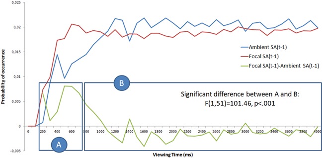
The probability of occurrence of focal and ambient fixations as a function of viewing time. Probability density functions are computed by taking into account the number of focal and ambient visual fixations. Two clusters were identified: cluster A (< 700 ms), which has more focal than ambient fixations, and cluster B (> 700ms), which shows no difference between focal and ambient fixations.
Figure 5.
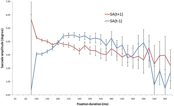
Median saccade amplitude and 95% confidence intervals as a function of the current fixation duration (FD(t)). The saccade amplitudes are derived from either the previous (SA(t − 1)) or the subsequent saccade (SA(t + 1)).
3. Results
The purpose of this study is to investigate whether two different modes of visual processing are employed while freely viewing a scene. Fixation durations and saccade amplitudes were first analysed separately as a function of the viewing time and were subsequently analysed together. Next, we applied an algorithm to classify the visual fixations.
3.1. Fixations and saccades
3.1.1. Fixation duration as a function of viewing time.
Figure 4a gives the median values of the fixation durations as a function of viewing time. As did Pannash et al (2008), we considered early, middle, and late visual processing periods. The early phase concerns the first 1.5 s of viewing, the middle phase corresponds to 1.5–3 s, and the late phase is the period of 3–4.5 s. We hypothesised that different contributions may occur sequentially during each phase. During the first phase, it is reasonable to assume that the contribution is mostly bottom-up. In later phases, the bottom-up contribution is likely to be progressively overridden by top-down influences (Parkhurst et al 2002). The extent to which these mechanisms contribute to gaze deployment, however, has yet to be determined.
Figure 4.
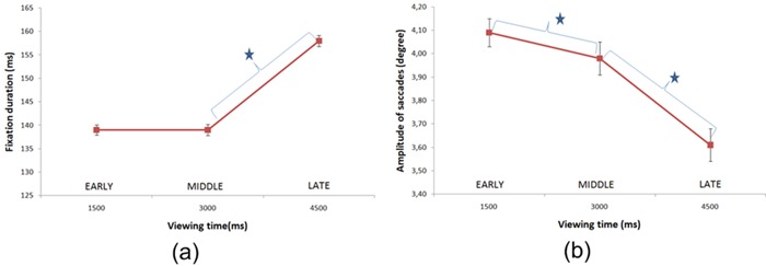
Median fixation duration (a) and saccade amplitude (b) as a function of viewing time. The error bars represent the 95% confidence interval. A star indicates a significant difference (Bonferroni-corrected t-test, p < .05).
We found that the median fixation duration increased with the viewing time. A one-way ANOVA using the factor of time (Early, Middle, Late) found a significant effect of time on the fixation duration (F(2,53446) = 11.2; p < .001). A bonferroni-corrected t-test found that the fixation durations during the Early and Middle periods were not significantly different (F(1,53446) = 5.28, p < .06)), but there was a significant difference between fixation durations during the Middle and Late periods (F(1,53446) = 5.88, p < .05).
This finding is similar to previous studies (Yarbus 1967; Antes 1974; Pannash et al 2008). Fixation durations are shorter immediately after the stimulus onset compared with those occurring after three seconds of viewing. This shift might be due to the contribution of bottom-up and top-down mechanisms. Immediately after the stimulus onset, our gaze is likely to be mostly driven by low-level visual features. The bottom-up aspect is an unconscious and fast mechanism. After several seconds of viewing, the top-down process becomes more influential on the way we process the visual information within a picture. At this later stage, our gaze is likely to be driven more by our own expectations and knowledge than by low-level visual features.
3.1.2. Saccade amplitude as a function of viewing time.
Figure 4b gives the median saccade amplitudes as a function of viewing time. As stated previously, there are three time periods: Early, Medium, and Late. Our results are consistent with previous studies (Yarbus 1967; Antes 1974; Pannash et al 2008). A one-way ANOVA found a significant interaction between saccade length and time (F(2,49721) = 57.68, p < .001). A bonferroni-corrected t-test found significant differences between Early/Middle (F(1,49721) = 113.2, p < .001) and Middle/Late (F(1,49721) = 14.02, p < .001) periods.
In summary, long saccades occur initially to allow rapid assessment of the visual content of the scene. The saccade amplitudes decrease over time, allowing focal inspection to be used to explore the scene in greater detail.
3.1.3. The relationship between fixation duration and saccade amplitude.
The two previous sections investigated the time course of fixation duration and saccade amplitude separately. Figure 5 gives the relationship between fixation durations and both previous and subsequent median saccade amplitudes. In this figure, it is difficult to classify visual fixations as one of the two types of visual processing. However, the saccade amplitude can be used to estimate the fixation duration (Velichkovsky et al 2005; Unema et al 2005). For instance, a saccade amplitude of 4 deg. of the visual angle might be used to categorise the visual fixations. To obtain an objective classification, an automated method was used to segment visual fixations into two groups. Note that the fixation durations and the saccade amplitudes were analysed conjointly. The method is described in the next section.
3.1.4. Classification using a k-means algorithm.
To verify the existence of two fixation types, a k-means clustering was used. This method is used to find clusters by partitioning n observations into k clusters, where each observation belongs to the cluster with the nearest mean. The algorithm iteratively moves the centre of each cluster to minimise the within-cluster sum of squares. It should be noted that each of the fixation durations and saccade amplitudes were standardised (z-scores) to address the problem of homoscedasticity (Figure 1 in Tatler et al 2006). However, even with this standardisation, violations of normality occurred (ie, skewed distribution). Consequently, we transformed the variables using the Box–Cox method. The Box–Cox method transforms the data (Osborne 2010), greatly reducing the skewness. After this transformation, our variables were close to a normal distribution (before transformation, skew (FD) = 1.49, skew (SA) = 1.21; after transformation, skew (FD) = 0.09, skew (SA) = −0.13). K-means clustering was carried out on both z-scores, and Box–Cox transformed data. The outcomes were notably similar (ie, same clusters).
Two clusters were used to identify the two modes of visual processing. Table 2 through Table 5 provide details regarding the clusters for each visual scene category. The results indicate that the relevant dimension for segmentation of data into two categories is the amplitude of the saccade. With the exception of the Mountain category, the two clusters were significantly different in terms of saccade amplitudes. For instance, there was a significant difference between clusters for the category Open Country (t(14077) = 168, p < .001). There is, however, no significant difference between clusters if the fixation durations is considered (t(14077) = 1.08, not significant for the category Open Country). These results are interesting for several reasons.
Table 2. Parameters of the clusters provided by the k-mean algorithm for the category, Open Country. ∗∗∗ indicates a significant difference (t-test, p < .001) between the cluster in term for FD or SA. (ns) indicates that differences were not significant.
| FD (ms) | SA(t − 1) | Number of cases | % | |
| Cluster 1 | 168.6 | 10.86 | 4,057 | 28.81 |
| Cluster 2 | 170.19(ns) | 2.52∗∗∗ | 10,022 | 71.18 |
| FD (ms) | SA(t + 1) | Number of cases | % | |
| Cluster 1 | 169.07 | 10.89 | 4,330 | 28.85 |
| Cluster 2 | 170.54(ns) | 2.51∗∗∗ | 10,678 | 71.14 |
Table 5. Parameters of the clusters provided by the k-mean algorithm for the category, Mountain. ∗∗∗ indicates a significant difference (t-test, p < .001) between the cluster in term for FD or SA. (ns) indicates that differences were not significant.
| FD (ms) | SA(t − 1) | Number of cases | % | |
| Cluster 1 | 172.84 | 11.01 | 4,072 | 28.73 |
| Cluster 2 | 164.77(ns) | 2.53∗∗∗ | 10,099 | 71.26 |
| FD (ms) | SA(t + 1) | Number of cases | % | |
| Cluster 1 | 164.85 | 11.05 | 4,299 | 28.49 |
| Cluster 2 | 168.99(ns) | 2.55∗∗∗ | 10,790 | 71.5 |
Table 3. Parameters of the clusters provided by the k-mean algorithm for the category Coast. ∗∗∗ indicates a significant difference (t-test, p < .001) between the cluster in term for FD or SA. (ns) indicates that differences were not significant.
| FD (ms) | SA(t − 1) | Number of cases | % | |
| Cluster 1 | 169.36 | 10.84 | 4,185 | 29.69 |
| Cluster 2 | 168.41(ns) | 2.47∗∗∗ | 9,907 | 70.3 |
| FD (ms) | SA(t + 1) | Number of cases | % | |
| Cluster 1 | 167.9 | 10.92 | 4,428 | 29.49 |
| Cluster 2 | 170.03(ns) | 2.47∗∗∗ | 10,587 | 70.50 |
Table 4. Parameters of the clusters provided by the k-mean algorithm for the category, Street. ∗∗∗ indicates a significant difference (t-test, p < .001) between the cluster in term for FD or SA. (ns) indicates that differences were not significant.
| FD (ms) | SA(t − 1) | Number of cases | % | |
| Cluster 1 | 167.93 | 11.18 | 3,954 | 26.96 |
| Cluster 2 | 169.41(ns) | 2.49∗∗∗ | 10,708 | 73.03 |
| FD (ms) | SA(t + 1) | Number of cases | % | |
| Cluster 1 | 169.41 | 11.2 | 4,223 | 27.05 |
| Cluster 2 | 169.64(ns) | 2.47∗∗∗ | 11,388 | 72.94 |
First, the two clusters may represent the focal and ambient fixation types. Indeed, the first cluster probably represents a focal processing mode; the saccade amplitudes are relatively small (Mean = 2.5°) compared with those of the second cluster (Mean = 10.5°) that may correspond to the ambient mode. Second, the populations of the two clusters are dramatically different. There is an average 70% and 30% of focal and ambient visual fixations in clusters 1 and 2, respectively. This population difference is congruent with the assumed role of ambient and focal visual modes. The former might be used to extract the overall layout of the scene and sample the scene to extract sparse local patches. From these dispersed patches we can infer fundamental information about the visual scene, such as its type. Contrary to the ambient fixations, the focal mode might be used to perform an accurate inspection of a small area. Several fixations would be required for inspection. Thus, a decrease in saccade amplitude probably indicates a period of ‘local’ fixations. Third, the clustering is nearly identical regardless of the scene category. This finding suggests that the visual fixation dichotomy is independent of the visual scene type. This systematic tendency might underline an automatic viewing process that is linked to the motor aspects of visual attention (Rizzolatti et al 1987). Fourth, the automatic clustering shows identical centroids when both the subsequent and previous saccade amplitudes are analysed. However, the meaning of these two configurations is different. Indeed, if we want to label fixations as focal or ambient, it makes more sense to consider the previous saccade amplitude than the subsequent one. A fixation preceded by a small saccade would be labelled as focal, whereas an ambient fixation is characterised by a longer previous saccade.
3.1.5. The time course of ambient and focal visual fixations.
Two populations of visual fixations were identified. In this section we focus on the time course of ambient and focal visual fixations. Previous studies (Unema et al 2005; Irwin and Zelinsky 2002; Tatler and Vincent 2008) found that the ambient mode primarily occurs at the onset of viewing, whereas the focal mode begins several milliseconds after the onset of viewing. To address this point, the probability of occurrence of focal and ambient fixations was computed as a function of time. A histogram was then built for each population obtained from the k-means clustering. The bins shown in the histogram represent the viewing time. For each 100 ms bin, we counted the number of fixations. Two probability density functions, including one for the focal cluster and another for the ambient cluster, were subsequently obtained by dividing the population of each bin by the total number of fixations. Figure 6 shows the probability density functions (pdf) for the ambient and focal fixations according to the viewing time. This measure reveals the probability that an ambient or focal fixation will occur at any given time.
Our results indicate that there is a dominance of focal fixations immediately after the stimuli onset. By analysing the difference between the probability of occurrences of such fixations (green curve in Figure 6), a significant difference was observed between the focal and ambient probabilities. Using k-means, two time intervals were identified (Figure 6): the first (a) consists of fixations occurring before 700 ms, while the second (b) is composed of fixations occurring after 700 ms. The difference between the two intervals was significant, (F(1,51) = 101.46, p < .001). The pdf of focal fixations increased up to 600 ms, staying almost constant over time thereafter (average ± standard deviation = 0.019 ± 0.00076).
Figure 6 shows the probability of the occurrence of focal or ambient fixations over time. To directly compare the contributions of each population over time, two probability density functions were calculated by dividing each bin of the focal and ambient fixations histogram by the total number of visual fixations (ie, the sum of focal and ambient fixations; see Figure 7). The results indicate that the ambient mode contribution increases up to 1,000 ms before reaching an asymptote.
Figure 7.
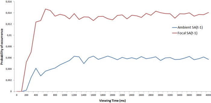
The probability of the occurrence of focal and ambient fixations as a function of viewing time. Probability density functions take into account the total number of visual fixations.
This result is not consistent with previous studies (Irwin and Zelinsky 2002; Unema et al 2005; Tatler and Vincent 2008) in which the ambient mode was dominant during the beginning of the viewing period. Our results also indicate that the ambient mode is present after several seconds of viewing and that the two populations of visual fixations are mixed together, suggesting an interplay between the modes (Pannasch et al 2008).
3.1.6. Summary.
Using an automated classification, we found that the previous saccade amplitude can be used to classify the visual fixations into two statistically distinguishable clusters. Furthermore, the fixation duration is not required to cluster the data. Two centroids were found: a first centroid is centred at 2.5 deg. and the second at about 11 deg. The former might be related to the focal mode, whereas the latter probably represents the ambient mode. This finding is conserved across the four visual scene categories. As these categories represent a range of stimuli, this kind of classification is probably a systematic and fundamental phenomenon. It is difficult, however, to interpret the role of each visual mode. A parallel might be drawn between the focal–ambient dichotomy and bottom-up versus top-down visual attention. To investigate the extent to which the focal mode is bottom-up, the degree of similarity between saliency maps stemming from computational models of the bottom-up visual attention and focal (and ambient) saliency maps was assessed.
4. Focal and ambient saliency maps
4.1. Fixation and saliency map of focal and ambient processing
Visual fixations were labelled as either focal or ambient based on the amplitude of the preceding saccade. The fixation type was determined by comparing the amplitude of the current saccade with the average saccade amplitude of the two clusters. If the distance between the centre of the focal cluster and the current saccade amplitude is smaller than the distance between the centre of the ambient cluster and the current amplitude of saccade, then the fixation is labelled focal. Otherwise, the fixation is labelled ambient. Note that the fixation duration was not used because this dimension does not significantly affect clustering.
4.2. Comparison between focal–ambient maps and computational saliency maps
There were considerable differences between focal and ambient fixation maps (Figure 8); therefore, a comparison between these maps and computational maps was carried out in order to test the relevance of our assumption that ambient processing is less bottom-up than the focal processing. The robustness of the comparison is an important factor that should not be underestimated. To be as independent as possible of the limitations of a particular model, four different computational models were used to compute saliency maps. The first three models, Itti (Itti et al 1998), Le Meur (Le Meur et al 2006), and Bruce (Bruce and Tsotsos 2009), rely on two seminal works: the biologically plausible architecture for controlling bottom-up attention that was proposed by Koch and Ullman (1985) and the Feature Integration Theory (Treisman and Gelade 1980) that posits that visual processing is able to encode visual features, such as colour, form, and orientation, in a parallel manner. The major distinguishing feature of Bruce's model is the probabilistic framework used to derive the saliency. The last model is Judd's model (Judd et al 2009), which is derived from a large database of eye-tracking data. When compared with the others, this model includes higher level information, such as the position of the horizon line, human faces, detection of cars and pedestrians, and a feature indicating the distance of each pixel from the centre. Previous studies (Le Meur et al 2006; Tatler 2007; Bindemann 2010) noted a bias toward the centre of the screen; therefore, a centred model was also used. The maximum value of 1 is located at the picture's centre, with values decreasing with increasing eccentricity. For example, a value of 0.5 is obtained at a 3.5 deg. visual angle.
Figure 8.
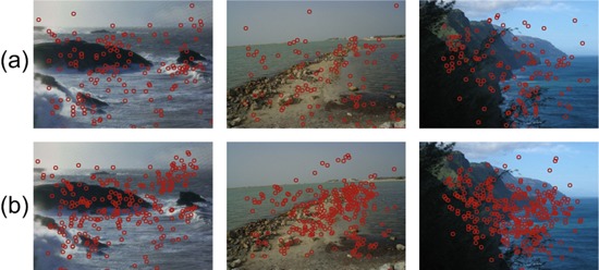
Ambient (a) and focal (b) fixation maps.
Finally, a random model was designed. The input of the model is the saliency map computed by Judd's model. The random model then randomises the input map into non-overlapping 32 pixels × 32 pixels blocks. Figure 9 shows the predicted saliency maps computed using the different models. Bright areas correspond to the most salient locations.
Figure 9.

Predicted saliency maps obtained from different models. (a) Original picture, (b) Itti's model, (c) Le Meur's model, (d) Bruce's model, (e) Judd's model, and (f) random model.
To quantify the degree of similarity between predicted saliency maps and experimental maps (focal or ambient), an ROC analysis was conducted (Fawcett 2006; Le Meur and Chevet 2010). Pixels were labelled as being fixated or not. The ROC analysis provides a curve that plots the false alarm rate (labelling a non-fixated location as fixated) as a function of the hit rate (labelling fixated locations as fixated). The binarised focal/ambient maps are used as a reference. A fixed threshold was chosen to keep, on average, the top 20% of salient locations. Other thresholds (5%, 10%, and 15%) were tested with similar results. Thresholds that are uniformly distributed between the minimum and maximum values of the predicted maps were used to label the pixels of the predicted maps. A perfect similarity between two maps results in an Area Under the Curve (AUC) equal to 1. An AUC of 0.5 suggests that the similarity is at the chance level. Figure 10 shows the ambient and focal maps after the threshold operation for a given picture.
Figure 10.

(a) Original picture; (b) Ambient map thresholded to keep the most fixated areas of the images (around 20%); (c) focal map thresholded to keep the most fixated areas of the images (around 20%).
Figure 11 shows the median AUC for the different models. AUC values were higher for the focal maps than for the ambient maps. Except for the random and Bruce's model, the differences between the focal and ambient maps were statistically significant (paired t-test). The statistics are reported in the figure. Focal maps were better predicted by saliency models than were ambient ones. These results are consistent with the assumption that ambient processing is less bottom-up than focal processing, supporting the hypothesis that the ambient process is more concerned with the scene layout. The three bottom-up models (Itti's, Le Meur's, and Judd's model) give better results when the focal map is used for the comparison. The ambient mode is also bottom-up but to a lesser extent. This finding is consistent with previous studies (Tatler et al 2006; Rajashekar et al 2007) that report large saccades are less dependent on low-level visual features than are short saccades. Because the ambient mode is used to quickly explore and identify the scene's most interesting regions, it is likely to behave as a random mode and be less dependent on low-level visual features. The comparison with a random model, however, rules out the idea that ambient visual fixations are purely random. Our results indicate that the overall prediction is significantly better than chance (p < .001), suggesting that both visual processing modes are driven by the low-level visual features to some extent and that the ambient mode is not based on a random sampling.
Figure 11.

Area Under the Curve (AUC) values indicating the difference between computational saliency maps (models of Itti, Le Meur, Bruce, Judd) and focal (or ambient) maps. A value of 0.50 indicates random performance, whereas 1.00 denotes a perfect relationship. Error bars indicate the standard error of the mean.
It is also important to consider the role of the central bias. Compared with the centre model, the magnitude of the AUC obtained from focal maps is significantly higher than that obtained from ambient processing (paired t-test, p < .001). We already knew that the screen's centre plays an important role in visual attention deployment and that a centred Gaussian model often provides better quantitative performance than computational saliency maps (Le Meur et al 2006). A number of factors can explain this central tendency. The centre might reflect an advantageous viewing position for extracting visual information (see Tatler 2007; Renninger et al 2007). Tatler (2007) found that this central tendency was not significantly affected by the distribution of visual features in a scene. More recently, Bindemann (2010) showed that this central bias is not removed by offsetting scenes from the screen's centre, varying the location of a fixation marker preceding the stimulus onset or manipulating the relative salience of the screen. Bindemann concluded that the screen-based central fixation bias might be an inescapable feature of scene viewing under laboratory conditions. These issues are consistent with our hypothesis. Ambient maps are less predicted by the centred model, suggesting that the screen's centre is more neglected in the ambient mode than in the focal mode. Positions farthest from the centre would be more favoured in the ambient mode. Based on these observations, two preliminary conclusions can be drawn:
-
1.
Focal maps are more bottom-up than ambient maps;
-
2.
The degree of similarity between focal and centred maps is significantly higher in the ambient map compared with the centred map. This second conclusion is consistent with previous studies (Tatler et al 2006; Rajashekar et al 2007).
As the focal and ambient visual processing modes depend on the viewing time (see Figure 6), the degree of similarity between computational and experimental maps was computed based on the first two and last two seconds. Figure 13 and Figure 14 show the results of this analysis. All statistics are reported in the figure. Our results indicate that the centred model has a strong impact during the early phase (0 to 2s). The contribution of this model dramatically decreases during late ambient fixations (2s to 4s) but increases during late focal fixations. This finding confirms the hypothesis that focal fixations are more centred than ambient ones. However, it is important to emphasise that ambient fixations in the early phase are also predicted by the centre model. This finding is more or less consistent with our first hypothesis. Indeed, we assume that the ambient mode is used to make a large-scale exploration of the scene, especially immediately after the stimulus onset. Our results suggest that the exploration scale during the first two seconds is not as large as we would expect. The exploration seems to be restricted to an area located around the centre of screen. However, regarding the late phase, the degree of similarity between late ambient map and centred map dramatically decreases, a finding that is consistent with our preliminary hypothesis. Figure 12 shows the amplitude of previous saccades for two temporal phases: the early phase, corresponding to the 0–2 s interval, and the late phase, corresponding to the 2–4 s interval. Interestingly, the median amplitude of saccades significantly increases with viewing time for the ambient mode (F(1,11114) = 138, p < .001). This finding is not consistent with previous findings (Figure 4) where there was a decrease in saccade amplitude with increased viewing time. Thus, just after the stimulus onset, scene exploration might start locally (ie, small saccades), becoming more global (longer saccades) over time. This local-to-global behaviour is consistent with the results obtained by the centre model on Figure 13. This trend might reflect the efforts used to explore the scene. After the stimuli onset, the visual inspection would concern the periphery of the screen's centre, whereas, after several seconds, the visual inspection would extend outward.
Figure 13.

Area Under the Curve between early and late ambient saliency maps and computational saliency maps.
Figure 14.

Area Under the Curve between early and late focal saliency maps and computational saliency maps.
Figure 12.

The median amplitude of previous saccades for the two modes of visual processing as a function of the viewing time. The left-hand side shows ambient fixations (a), and the right-hand side shows focal fixations (b).
Finally, the conclusion that the focal mode is more bottom-up than the ambient mode is consistent with results shown in Figure 13 and Figure 14. Regardless of the phase, focal maps are influenced more heavily by bottom-up processing than are ambient maps.
5. Discussion and conclusions
The present study investigated the existence of two different populations of visual fixations. We examined the relationship between fixation durations and saccade amplitudes (Unema et al 2005). This relationship is non-linear and time dependent, thereby suggesting the existence of two kinds of visual fixations. Using this observation, visual fixations were classified, and their relation to computational saliency was investigated. Our findings are addressed below.
5.1. Two visual fixation populations
Visual fixations were first classified using a k-means clustering algorithm, and it was found that the saccade amplitude is the determining feature for clustering. The first cluster groups visual fixations that are characterised by small saccade amplitudes (average = 2.5 deg.), whereas the second cluster groups fixations with larger saccade amplitudes (average = 11 deg.). Our results confirm the existence of two visual processes (Trevarthen 1968; Unema et al 2005; Pannasch et al 2008); the first cluster represents the focal visual process used to accurately inspect areas, while the second cluster represents ambient fixations that are used to explore the visual field. Similar to previous studies (Unema et al 2005), we observed a larger proportion of focal fixations; approximately 70% of the visual fixations were labelled focal. This result is consistent with the fixations' presumed role in visual processing. Importantly, this finding was consistent across scene categories.
5.2. A different sensibility to the central tendency
The second conclusion concerns the central fixation bias. In this study the central fixation bias was observed immediately after the stimuli onset for both populations of visual fixations. Even ambient fixations that are used to explore the scene are located near the centre. However, ambient fixations become less dependent on the central tendency as the viewing time increases. This temporal behaviour might reflect a local-to-global scene strategy. Scene exploration might start near the centre and subsequently extend to locations far from the scene's centre. In other words, the screen's centre might be a good place to begin further exploration of the scene. With regard to focal fixations, an opposite effect was observed over time; the central fixation bias was more pronounced after 2 s of viewing. These observations confirm the importance of the scene's centre. The increase in the central bias contribution might be related to two important features illustrated in previous studies. First, fixation locations correlate with low-level visual features (Reinagel and Zador 1999; Parkhurst et al 2002; Tatler et al 2005), and second, interesting features are often located in the centre of natural scenes (ie, photographers tend to place objects of interest at the centre of the picture).
5.3. Time course of focal and ambient fixations
The third conclusion concerns the time course of focal and ambient fixations. There are few studies concerning this subject. Ambient processing is believed to occur primarily just after stimulus onset with the focal mode coming into play later on (Pannasch et al 2008; Unema et al 2005; Norman 2002). Our results, however, are not consistent with these previous studies. We observed that the focal mode is the most important mode over time and occurs immediately after stimulus onset. This result may be explained by the central bias. Indeed, immediately after the stimulus onset, the screen's centre attracts our attention for several reasons that have been mentioned previously. This phase is considered, in our classification, to be a focal one. The contribution of the ambient mode also increases over time but not as rapidly as the focal mode. It reaches its maximal influence after 1 s, thereafter remaining at a nearly constant rate.
5.4. Are focal and ambient visual fixations bottom-up?
The role of focal and ambient fixations was also investigated. The focal mode is more dependent on low-level visual features than is the ambient mode. This conclusion was derived from the comparison between focal and ambient maps and predicted saliency maps. Special consideration has to be given to this interpretation. For instance, the focal mode can be considered, in our study, to be more related to a bottom-up model than the ambient one simply because of the central bias or high-level object understanding. The latter explanation is supported by recent studies (Elazary and Itti 2008; Le Meur and Chevet 2010; Masciocchi et al 2009) suggesting that bottom-up models are good predictors of interesting hand-label regions of a scene. Although purely based on bottom-up features, bottom-up models successfully predict areas of interest that are consciously chosen by observers. This finding suggests that computational saliency models predict fixations based on bottom-up features but also, to some extent, fixations that are based on higher-level information. To further investigate the role of ambient and focal fixations, it would be interesting to combine several sets of behavioural data. Future studies could use the EFRP technique (Baccino 2011) that combines EEGs with eye-tracking. EFRPs are extracted from EEGs by averaging the brainwaves occurring during the onset and offset of eye-fixation. Analysis of EFRP components may reveal the time course of attention or semantic processing. Separating these components with statistical procedures and the localisation of the activation may be highly informative for the labelling of fixations. These findings would significantly contribute to the interpretation of scan paths and fixations during real-life activities. For example, EFRPs are useful for the investigation of early lexical processes and for establishing a timeline of these processes during reading (Baccino and Manunta 2005) or during object identification (Rama and Baccino 2010).
5.5. The duration of fixation is not a discriminant factor
Finally, we would like to emphasise our results regarding fixation duration. It is generally believed that fixation duration reflects the depth of processing (Velichkovsky 2002) and the ease or difficulty of information processing. This behaviour has been demonstrated when observers look at a picture (Mannan et al 1995) or read a text (Daneman and Carpenter 1980). Here, we found that fixation duration is not useful for classifying visual fixations into clusters. However, if the focal mode relies on top-down visual processing, it probably involves cognitive mechanisms, and the duration of focal fixations will probably be higher than that of ambient fixations. How can we explain why the duration of fixation does not play an important role? It is possible that this result is due to the lack of a task or goal in the present study. Indeed, task-free viewing requires the examination of the spatial environment and the casual observation of the picture. The ‘relevance’ of fixation durations would also depend on the material used.
Biography
Brice Follet received his master degree in cognitive sciences from the INP Grenoble in 2005. He is a PhD student from the collaboration between Technicolor R & I and University of Paris 8. He investigates the functional roles and correlates of ambient and focal fixations.
 Olivier Le Meur obtained his PhD degree from the University of Nantes in 2005. From 1999 to 2009, he has worked for ten years in the media and broadcasting industry. In 2003 he joined the research center of Thomson-Technicolor at Rennes where he supervised a research project concerning the modelling of the human visual attention. Since 2009 he has been an associat professor for image processing at the University of Rennes 1. In the IRISA/TEMICS team his research interests are dealing with the understanding of the human visual attention. It includes computational modelling of the visual attention and saliency-based applications (video compression, objective assessment of video quality, retargeting). Home page: http://www.irisa.fr/temics/staff/lemeur.
 Thierry Baccino is full-professor of Cognitive Psychology in Digital Technologies at the University of Paris 8 and scientific director of LUTIN (CNRS-UMS 2809) located at the National Museum of Sciences and Techniques in Paris. He obtained his PhD in cognitive psychology from the University of Aix-en-Provence in 1991, having been granted by National IBM Research Centre. He became assistant professor at the University of Nice Sophia-Antipolis (UNS) in 1993 and full-professor in 1998. After several visiting professorships (Pavia, Dortmund, Torino), he received in 2004 a Fulbright award for working at the Institute for Cognitive Science (University of Colorado at Boulder, USA). He is currently scientific expert at the European DG Research and at different French research institutes (ANR, AERES). His research focus is mainly on reading and information seeking using both experimental methods (especially eye-tracking and eye-fixation-related potentials) and computational modeling techniques.
Contributor Information
Brice Follet, Technicolor, 1 avenue Belle Fontaine, 35510 Cesson-Sévigné, France; e-mail: Brice.Follet@technicolor.com.
Olivier Le Meur, Université de Rennes 1—IRISA, Campus Universitaire de Beaulieu, 35042 Rennes Cedex, France; e-mail: olemeur@irisa.fr.
Thierry Baccino, LUTIN, Cité des sciences et de l'industrie de la Villette, 30 avenue Corentin Cariou, 75930 Paris Cedex 19, France; e-mail: thierry.baccino@univ-paris8.fr.
References
- Antes J R. “The time course of picture viewing”. Journal of Experimental Psychology. 1974;103:62–70. doi: 10.1037/h0036799. [DOI] [PubMed] [Google Scholar]
- Baccino T. “Eye Movements and concurrent ERP's: EFRPs investigations in reading”. In: Liversedge S, Gilchrist Ian D, Everling S, editors. Handbook on Eye Movements. Oxford, UK: Oxford University Press; 2011. pp. 857–870. [Google Scholar]
- Baccino T, Manunta Y. “Eye-Fixation-Related Potentials: Insight into Parafoveal Processing”. Journal of Psychophysiology. 2005;19:204–215. doi: 10.1027/0269-8803.19.3.204. [DOI] [Google Scholar]
- Bindemann M. “Scene and screen center bias early eye movements in scene viewing”. Vision Research; 2010. [DOI] [PubMed] [Google Scholar]
- Bruce N D B, Tsotsos J K. “Saliency, attention and visual search: an information theoretic approach”. Journal of Vision. 2009;9:1–24. doi: 10.1167/9.3.5. [DOI] [PubMed] [Google Scholar]
- Daneman M, Carpenter P A. “Individual differences in working memory and reading”. Journal of Verbal Learning and Verbal Behavior. 1980;19:450–466. doi: 10.1016/S0022-5371(80)90312-6. [DOI] [Google Scholar]
- Elazary L, Itti L. “Interesting objects are visually salient”. Jounrnal of Vision. 2008;7(3):1–15. doi: 10.1167/8.3.3. [DOI] [PubMed] [Google Scholar]
- Fawcett T. “An introduction to ROC analysis”. Pattern Recognition Letters. 2006;27:861–874. doi: 10.1016/j.patrec.2005.10.010. [DOI] [Google Scholar]
- Findlay J M, Gilchrist I D. “Active vision: the psychology of looking and seeing”. Oxford, UK: Oxford University Press; 2003. [Google Scholar]
- Follet B, Le Meur O, Baccino T. “Modeling visual attention on scenes”. Studia Informatica Universalis. 2010;8:150–167. [Google Scholar]
- Harding G, Bloj M. “Real and predicted influence of image manipulations on eye movements during scene recognition”. Journal of Vision. 2010;10:2–2. doi: 10.1167/10.2.8. [DOI] [PubMed] [Google Scholar]
- Henderson J M, Pierce G L. “Eye movements during scene viewing: Evidence for mixed control of fixation durations”. Psychonomic Bulletin & Review. 2008;15:566–573. doi: 10.3758/PBR.15.3.566. [DOI] [PubMed] [Google Scholar]
- Irwin D E, Zelinsky G J. “Eye movements and scene perception: memory for things observed”. Perception & Psychophysics. 2002;64:882–895. doi: 10.3758/BF03196793. [DOI] [PubMed] [Google Scholar]
- Itti L, Koch C, Niebur E. “A model for saliency-based visual attention for rapid scene analysis”. IEEE Transactions on Pattern Analysis and Machine Intelligence. 1998;20:1254–1259. doi: 10.1109/34.730558. [DOI] [Google Scholar]
- Judd T, Ehinger K, Durand F, Torralba A. “Learning to Predict Where Humans Look”. ICCV; 2009. [Google Scholar]
- Koch C, Ullman S. “Shifts in selective visual attention: towards the underlying neural circuitry”. Human Neurobiology. 1985;4:219–227. [PubMed] [Google Scholar]
- Norman J. “Two visual systems and two theories of perception: an attempt to reconcile the constructivist and ecological approaches”. Behavioral and Brain Sciences. 2002;25:73–144. doi: 10.1017/s0140525x0200002x. [DOI] [PubMed] [Google Scholar]
- Le Meur O, Le Callet P, Barba D, Thoreau D. “A coherent computational approach to model the bottom-up visual attention”. IEEE Transactions on Pattern Analysis and Machine Intelligence. 2006;28:802–817. doi: 10.1109/TPAMI.2006.86. [DOI] [PubMed] [Google Scholar]
- Le Meur O, Chevet J C. “Relevance of a feed-forward model of visual attention for goal-oriented and free-viewing tasks”. IEEE Transactions on Image Processing. 2010;19:2801–2813. doi: 10.1109/TIP.2010.2052262. [DOI] [PubMed] [Google Scholar]
- Le Meur O, Ninassi A, Le Callet P, Barba D. “Overt visual attention for free-viewing and quality assessment tasks. Impact of the regions of interest on a video quality metric”. Signal Processing: Image Communication. 2010;25:547–558. doi: 10.1016/j.image.2010.05.006. [DOI] [Google Scholar]
- Mannan S, Ruddock K H, Wooding D S. “Automatic control of saccadic eye movements made in visual inspection of briefly presented 2D images”. Spatial Vision. 1995;9:363–386. doi: 10.1163/156856895X00052. [DOI] [PubMed] [Google Scholar]
- Masciocchi C M, Mihalas S, Parkhurst D, Niebur E. “Everyone knows what is interesting: salient locations which should be fixated”. Journal of Vision. 2009;9:11–11. doi: 10.1167/9.11.25. [DOI] [PMC free article] [PubMed] [Google Scholar]
- Oliva A, Schyns P G.2000“Colored diagnostic blobs mediate scene recognition” Cognitive Psychology 2000 [DOI] [PubMed]
- Osborne J W. “Improving your data transformations: Applying the Box-Cox transformation. Practical Assessment”. Research & Evaluation. 2010;15:1–7. [Google Scholar]
- Over E A B, Hooge I T C, Vlaskamp B N S, Erkelens C J. “Coarse-to-fine eye movement strategy in visual search”. Vision Research. 2007;47:2272–2280. doi: 10.1016/j.visres.2007.05.002. [DOI] [PubMed] [Google Scholar]
- Pannasch S, Helmert J R, Roth K A K, Walter H. “Visual Fixation Durations and Saccade Amplitudes: Shifting Relationship in a Variety of Conditions”. Journal of Eye Movement Research. 2008;2:1–19. [Google Scholar]
- Pannasch S, Velichkovsky B M. “Distractor Effect and Saccade Amplitudes: Further Evidence on Different Modes of Processing in Free Exploration of Visual Images”. Visual Cognition. 2009;17:1109–1131. doi: 10.1080/13506280902764422. [DOI] [Google Scholar]
- Parkhurst D, Law K, Niebur E. “Modelling the role of salience in the allocation of overt visual attention”. Vision Research. 2002;42:107–123. doi: 10.1016/S0042-6989(01)00250-4. [DOI] [PubMed] [Google Scholar]
- Rajashekar U, Van der Linde I, Bovik A C. “Foveated analysis of image features at fixations”. Vision Research. 2007;47:3160–3172. doi: 10.1016/j.visres.2007.07.015. [DOI] [PubMed] [Google Scholar]
- Rama P, Baccino T. “Eye-fixation related potentials (EFRPs) during object identification”. Visual Neuroscience. 2010;27:1–6. doi: 10.1017/S0952523810000283. [DOI] [PubMed] [Google Scholar]
- Reinagel P, Zador A M. “Natural scene statistics at the centre of gaze”. Network: Computation in Neural Systems. 1999;10:341–350. doi: 10.1088/0954-898X/10/4/304. [DOI] [PubMed] [Google Scholar]
- Renninger L W, Vergheese P, Coughlan J. “Where to look next? Eye movements reduce local uncertainty”. Journal of Vision. 2007;7:1–17. doi: 10.1167/7.3.6. [DOI] [PubMed] [Google Scholar]
- Rizzolatti G, Riggio L, Dascola I, Umilta C. “Reorienting attention across the horizontal and vertical meridians: evidence in favor of a premotor theory of attention”. Neuropsychologia. 1987;25:31–40. doi: 10.1016/0028-3932(87)90041-8. [DOI] [PubMed] [Google Scholar]
- Scinto L F, Pillalamarri R, Karsh R. “Cognitive strategies for visual search”. Acta Psychologica. 1986;62:263–292. doi: 10.1016/0001-6918(86)90091-0. [DOI] [PubMed] [Google Scholar]
- Schyns P G, Oliva A. “From blobs to boundary edges: Evidence for time- and spatial-scale-dependent scene recognition”. Psychological Science. 1994;5:195–200. doi: 10.1111/j.1467-9280.1994.tb00500.x. [DOI] [Google Scholar]
- Tatler B W, Baddeley R J, Gilchrist I D. “Visual correlates of fixation selection: Effects of scale and time”. Vision Research. 2005;45:643–659. doi: 10.1016/j.visres.2004.09.017. [DOI] [PubMed] [Google Scholar]
- Tatler B W, Baddeley R J, Vincent B T. “The long and the short of it: spatial statistics at fixation vary with saccade amplitude and task”. Vision Research. 2006;46:1857–1862. doi: 10.1016/j.visres.2005.12.005. [DOI] [PubMed] [Google Scholar]
- Tatler B W. “The central fixation bias in scene viewing: Selecting an optimal viewing position independently of motor biases and image feature distributions”. Journal of Vision. 2007;7:1–17. doi: 10.1167/7.14.4. [DOI] [PubMed] [Google Scholar]
- Tatler B W, Vincent B. “Systematic tendencies in scene viewing”. Journal of Eye Movement Research. 2008;2:1–18. [Google Scholar]
- Torralba A, Oliva A. “Modeling the shape of the scene: a holistic representation of the spatial envelope”. International Journal of Computer Vision. 2001;42:145–175. doi: 10.1023/A:1011139631724. [DOI] [Google Scholar]
- Treisman A, Gelade G. “A feature-integration theory of attention”. textit{Cognitive Psychology} 1980;12:97–136. doi: 10.1016/0010-0285(80)90005-5. [DOI] [PubMed] [Google Scholar]
- Trevarthen C B. “Two mechanisms of vision in primates”. Psychologische Forschung. 1968;31:299–337. doi: 10.1007/BF00422717. [DOI] [PubMed] [Google Scholar]
- Unema P J A, Pannasch S, Joos M, Velichkovsky B M. “Time course of information processing during scene perception: The relationship between saccade amplitude and fixation duration”. Visual Cognition. 2005;12:473–494. doi: 10.1080/13506280444000409. [DOI] [Google Scholar]
- Velichkovsky B M. “Heterarchy of cognition: The depths and the highs of a framework for memory research”. Memory. 2002;10:405–419. doi: 10.1080/09658210244000234. [DOI] [PubMed] [Google Scholar]
- Velichkovsky B M, Joos M, Helmert J R, Pannasch S.2005“Two visual systems and their eye movements: evidence from static and dynamic scene perception” Proceedings of the XXVII conference of the cognitive science society, 2283–2288.
- Yarbus A L. Eye Movements and Vision. New York: Plenum Press; 1967. [Google Scholar]