Rank order scaling of pictorial depth

Abstract

We address the topic of “pictorial depth” in cases of pictures that are unlike photographic renderings. The most basic measure of “depth” is no doubt that of depth order. We establish depth order through the pairwise depth-comparison method, involving all pairs from a set of 49 fiducial points. The pictorial space for this study was evoked by a capriccio (imaginary landscape) by Francesco Guardi (1712–1793). In such a drawing pictorial space is suggested by the artist through a small set of conventional depth cues. As a result typical Western observers tend to agree largely in their visual awareness when looking at such art. We rank depths for locations that are not on a single surface and far apart in pictorial space. We find that observers resolve about 40 distinct depth layers and agree largely in this. From a previous experiment we have metrical data for the same observers. The rank correlations between the results are high. Perhaps surprisingly, we find no correlation between the number of distinct depth layers and the total metrical depth range. Thus, the relation between subjective magnitude and discrimination threshold fails to hold for pictorial depth.

1. Introduction

For the human observer “pictures” (roughly defined as a simultaneous order of colours in two dimensions) may give rise to a number of categorically different modes of experience (Gombrich 1960).

The most basic mode is that of the awareness of the picture as a physical object (Denis 2000), such as a piece of paper, a framed painting, the screen of a laptop computer or television set, a billboard, and so forth. In this mode pictures may have sizes and weights; they can sometimes be attached to walls, sometimes be carried about, stored in cupboards, switched off, and more. That is to say, it is the mode that enables efficacious physical interaction. This mode humans doubtless share with many animals, not just primates. Applied to the perception of pictures, it is a mode that is perhaps more immediately familiar—or relevant—to removal contractors than it is to the general public, though. When people discuss their holiday snapshots, they as a matter of course talk of what is in these pictures, not about the physical properties of them.

In a different mode the human observer may be aware of a simultaneous spatial pattern. This pattern may be due to pigments distributed over a carrier, such as paints on a paper surface, a nexus of tiny luminous areas such as a computer desktop, and so forth. It does not really matter because the awareness is not focused on the physical structure at all but on the structural properties of the pattern, whatever its origin. Awareness of this type does not depend on whether the pattern is due to paints, LEDs, or something else. Examples include, but are in no way exhausted by, printed pages, Jackson Pollock's paintings, Times Square facade displays, and so forth. A painting is firstly a physical object, secondly a quilt of colors, thirdly something else (Denis 2000). Notice that we only consider pre-categorical awareness here. Thus, a printed page represents just another pattern, irrespective of whether one is able to “read the text.” In pre-categorical awareness, this mode of viewing is possibly shared by many animals, as familiar examples such as the “eyes” on butterfly wings suggest (Cott 1957; Wickler 1968). This mode is perhaps more immediately familiar to visual artists than it is to the general public, though.

Finally, the human observer may become aware of a “pictorial space” that magically appears when one “looks into” the picture. This mode of visual awareness is often thought to be specifically human, perhaps shared by some of the primates (Fagot 2001). It is this “default” mode that is immediately familiar to the general public. Pictorial space occurs spontaneously in many pictures that are unlike photographic renderings (eg, no central perspective, no preferred viewpoint), such as children's drawings or cubist paintings, and it therefore constitutes an interesting topic of research in itself.

Although it is often said that pictorial space “extends beyond the picture surface,” this has to be understood cum grano salis. Pictorial space is not a proper part of visual space; nor does it share the Euclidean structure with physical space. Pictorial spaces are figments of the mind, and their proper study belongs to psychology rather than geodesy. A remarkable difference between “physical space,” that is, the space you move in, and “pictorial space” is that your eye—and your body, of course—is not even located in pictorial space, whereas it definitely is part of physical space (Berkeley 1709; Wittgenstein 1921). This has many consequences of immediate importance to our work (for further discussion, see Koenderink et al 2011). For instance, pictorial objects have no “distance from the eye”; that very notion is void. Pictorial objects do have depth, but the depth domain has no natural origin, whereas the physical domain has. Your eye is the origin of physical space experienced from your perspective; it is as close as it gets. Although a key issue, this is rarely acknowledged in main-stream work, where the notion of a picture as a “window” is perhaps the more popular paradigm. The view through a window is connected to the space in front of the window which contains your eye, whereas pictorial space is not connected to physical space at all. It exists on a different ontological level, as discussed by Gibson (1950), Gombrich (1960), and Pirenne (1970).

The pictorial spaces explored most easily are those elicited by so called “realistic pictures” that are straight photographs of familiar scenes taken in a fairly standard manner—typical holiday snapshots, drawings and paintings in some “realistic style,” and so forth. It is by no means a requirement that the picture “depicts” any actual physical scene. Pictorial spaces occur readily when looking into pictures that depict science fiction or gothic scenes. In fact, they even occur when looking into random patterns, clouds, the image of Mars through a telescope, and so forth. This strongly suggests that pictorial space should be studied for its intrinsic interest, rather than as a substitute for something else. The study of the relation of pictorial spaces to certain physical spaces has many important applications, as in the valuation of “documentary photographs,” but this is a topic that stands clearly apart from the study of the structure of pictorial spaces as such.

Because pictorial space is a purely mental entity, the application of the familiar geodesic methods is ruled out. For instance, you cannot hold a yardstick next to a pictorial object so as to measure its length. More importantly, it is not even clear what meaning to attach to the “length of a pictorial object,” except when it happens to lie in the picture plane. The only viable approach is operational.

In the operational method one designs some scheme that intuitively addresses the topic of “pictorial length” and subsequently defines pictorial length as the result obtained by that scheme. Though no doubt a mean trick, pictorial entities can be formally handled only by way of such operational definitions. Although this holds equally true in the sciences, this is rarely acknowledged.

Such an understanding immediately leads to further problems. Suppose one has two or more operational definitions of pictorial length. This is a very common situation in experimental psychology. The two methods will most likely yield different results, occasionally leading to hot debates in the literature: Which one is right?

To ask the question “which one is right?” is to assume the objectivist stance. Pictorial length is assumed to possess an existence even in the absence of any measurement, and a “correct” measurement had better yield this result. Such an attitude often works in classical physics, for instance, if one measures the temperature of the water in a bucket one rightly expects a result that does not depend upon the thermometer one uses. If the results differ, then one or more of the thermometers must be defective. Such problems are rare. An example are the “ranges” used in astronomy. One strongly believes that all these ranges are actually one and the same, thus that there is an obvious answer to which one is right? When it turns out that one's trusted range measures are actually not equal, this causes a stir. It happened in the 1950s when Walter Baade reinterpreted the brightness of the Cepheid variables and thus changed one of the (then) trusted range measures (announced at the 1952 meeting of the International Astronomical Union in Rome). It doubled the diameter of our Milky Way at one fell swoop!

In psychology this works out differently. One has to adjust to the notion that the question “which one is right?” is not well posed. The reason is that pictures, even photographs, allow an infinite number of valid interpretations. Familiar examples are the Ames demonstrations (Ittelson 1952), especially the room and the chair. Confronted with photographs taken from Ames's intended position, observers commit spectacular errors as compared with the ground truth, which is exactly known in these cases. The point so forcefully made by Ames is that photographs do not come with intrinsic “ground truth”. The ground truth is known to the photographer, or may be revealed to others by verbal means, for instance. It is not available to the naive observer. It cannot be held that the naive observer is “wrong”, as the reported perceptions apply to scenes that might have produced the exact same photograph. Ames's point equally applies to drawings and paintings (Ames was an artist): if there is any ground truth, it is the intention of the artist, not necessarily known to the viewer.

Pictorial objects are mental constructions that need not even exist outside the context of an experiment. Different methods may very well induce different constructions (Koenderink and van Doorn 2003). Two distinct operationalizations should be expected to yield distinct results, even if both are labeled the same, say “pictorial length.” For such labels are assigned by the experimenter on intuitive grounds, they are not necessarily ontologically valid. Simply calling two distinct entities “length,” “depth,” and so on by no means magically forces their possibly different ontological roots to be equal. The formal relations between such operationalizations are properly a topic of empirical investigation.

In this paper we address the topic of “pictorial depth.” In a series of previous investigations we have explored various operationalizations of what is commonly referred to as pictorial depth. One result of these investigations is that human observers often come up with superficially very different results, which, on further analysis and perhaps surprisingly, turn out to be very similar when suitably transformed (Koenderink et al 2001). The transformations required appear to be entirely idiosyncratic, and a formal analysis suggests that they are due to the ambiguities common to virtually all “pictorial cues” (Koenderink and van Doorn 2008). The observer supplies a particular interpretation that is inside the set of all possible interpretations given the cues. Apparently, human observers generally use the same bouquet of cues.

A common transformation applied by observers is the dilation or contraction of the total depth range (Hildebrand 1901; Koenderink and van Doorn 2003). Here large differences are routinely encountered. Apparently, observers may experience very similar structures, as the very high correlations show (almost always more than 0.9, more typically more than 0.95), but spread out over very different ranges (Wagemans et al 2011). The total depth range seems to be idiosyncratic and is not correlated with differences in perceived structure. This gives rise to a number of questions that require further empirical study. Here we take a more refined look at possible differences in perceived structure.

In this paper we explore a method to measure ordinal depth structures in a conventional landscape painting. Our main objective is to forge an additional tool for research in pictorial perception. As argued above, it is desirable to build a toolbox with as many essentially different methods that all address the nominally same “depth” as possible. The present paper fits in this programme (for a more extensive review, see Koenderink et al 2011). In addition, we address some conceptual issues.

We selected a landscape painting of a non-existing scene (a “capriccio”) because it evidently has no “ground truth”, only a rather weakly implied perspective center (any viewpoint that is roughly central and neither extremely far from nor extremely close by the picture plane will do; the picture was never intended to be seen from a specific viewpoint). This is the generic case for most paintings in a roughly “realistic” style. The method will (as will any method) obviously have its limitations. For instance, neither Mondrian's nor Pollock's paintings would qualify as likely stimuli (of course, these hardly fall in the “realistic” category). However, the method applies easily to pictures that are not at all related to central projection; think of medieval woodprints, de Chirico's paintings, and so forth, for instance.

One of our aims is to discover whether observers that experience very different depth ranges have similar or correspondingly different depth resolution. The assumption that these properties are related is essentially due to Fechner (1860), although not originally formulated specifically for the depth domain. Specifically, Fechner's hypothesis is that the estimate of the depth gap between two points should stand in a monotonic relation to the number of just discriminable depth steps between these points.

Do observers that experience a shallow depth range resolve a similar number of depth slices as observers that experience an extended depth range, or rather a much smaller number? This is an issue that cannot be answered a priori but has to be decided empirically. The method explored here allows us to address this conceptually important question.

Another issue that we address is that of the very “existence” of pictorial space. In order for the concept of pictorial space to be of some utility, one requires it at least to be a consistent basis for the representation of actual observations. Because we attempt to account for more than a thousand observations in terms of only about 50 depth values, we are in an excellent position to address this issue.

2. Experiment

We adopt the conventional method of pairwise comparison (Cohn 1894; Wittmer 1894; Titchener 1901, 1908; Thurstone 1927, 1929, 1959; Kendall and Babington-Smith 1940; Kemeny 1959; Luce 1959) to find the ordinal distribution of depths in a pictorial space. In the past we have used similar methods to probe the structure of pictorial reliefs that are pictorial surfaces (Koenderink and van Doorn 1995; Koenderink et al 1996). Here we design a method that allows us to probe the structure of arbitrary point configurations. The stimulus we use is a realistic drawing of an imaginary landscape (Figure 1). Because it is a capriccio, “ground truth” is not available.

Figure 1.

The picture used as stimulus. This picture is a (close) copy of a wash drawing by Francesco Guardi (1712–1793), a capriccio (imaginary landscape with tower ruins and a fisherman's tent) by Anne-Sophie Bonno (http://www.atelier-bonno.fr/galerie-copies-arts-graphiques.html).

In order to use the method of pairwise comparison to probe depth resolution, it is desirable to apply it to a configuration consisting of a great many point pairs. This is the case because the position in the overall ranking of any single point will be co-determined by all the other points. The more points there are, the better any given point can potentially be localized. But because we require a full set of judgments, each point being compared with every other point, time constraints limit the size of feasible configurations. About 50 points—already implying more than a thousand pairwise judgments—is a realistic limit, even if every pair is presented only once. This implies that the two points of a pair should be presented in symmetrical fashion, such that balancing is not required (any asymmetry implies a doubling of the chore), placing an additional constraint on the implementation of the method. That all pairs are judged is necessary if the points are mutually unrelated in the sense that they are not on a single pictorial surface. In the latter case it is sufficient to judge pairs in small neighborhoods (Koenderink and van Doorn 1995; Koenderink et al 1996), rendering the total chore proportional to the number of points, instead of, as in the present (general) case, quadratic in the number of points.

Given a complete set of pairwise comparisons, one proceeds to construct a depth order that accounts for the observed judgments. Since there are a mighty ½N(N − 1) ≈ ½N² judgments for a mere N (more than a thousand for a mere 50) points, this is most of the time a practical impossibility. Thus, one attempts to find an order that “best” explains the observations in some reasonable sense. Because there are N! (more than 10⁶⁴ for 50 points) possible rank orders, this is not easily achieved by exhaustive search. In this study we use a simple voting method that yields results that are very stable against various perturbations. (See the Appendix.) In numerical simulations involving much fewer (up to ten) points, enabling one finding the exact set of “best” solutions, we found this voting method to be preferable. It is very stable against various types of random perturbations, including errors, such as hitting the wrong button by mistake, that tend to occur especially with naive observers, and very close in quality to the optimal solutions. The reason is that “optimal” applies only to a single session and thus is highly sensitive to singular occurrences (Schwartz 1972).

A decided advantage of this voting method is that it is a very intuitive one, enabling various heuristic methods to be brought into play easily.

A single session yields a particular depth order, as well as a subset of observations that fail to agree with that estimated depth order. These latter data evidently allow inferences to be made as to the mutual distinction of points with respect to depth. Unexplained observations are conventionally related to intransitivity, for instance, intransitive triads A, B, C such that A is nearer than B; B is nearer than C; and C, again, is nearer than A. This is often interpreted to indicate that A, B, and C should be considered to be effectively equidistant, an inference that is not a necessary one (Slater 1961; Tullock 1964). The voting method occasionally has to assign the same rank to some points. This turns out to be a rare occasion, though. One rarely encounters more than a few intransitive triangles in a session.

Repeated sessions yield a measure of the stability of the estimated rank order, and thus an estimate of the number of effectively resolved depth slices. In practice, one often ends up with a ranking that contains several runs of equidistant points, resulting in an effectively shrunken depth range, one shorter than the number of points N. It is the scatter in the estimated depth orders in relation to this range that can be interpreted in terms of a number of effectively resolved depth slices.

In order to be able to judge the depth order of a pair of points, these points need to be located in pictorial space—that means also in depth. This is not trivial since all one can do is place physical marks on the physical pictorial surface. One can only hope that these marks will be experienced as pictorial objects. Sometimes this fails to happen, as when one sees fly specks on the surface of a drawing. It is easy enough to bias the odds through shrewd choices of position in the picture plane and suitable design of the marks, though. As marks we use small—in relation to the size of the picture—circular dots of a color that contrasts with the general color of the picture. The latter constraint is necessary because the marks have to be reliably detected very fast. Such marks tend to “travel into depth” and attach themselves to pictorial objects if suitably positioned. For instance, they will attach readily to the nearest pictorial surface if there is one. They will also readily attach to small pictorial objects.

We placed marks at salient points defined by geographic and architectural details, human presence, and so forth. In no case did this result in the complaint that a point did not reside in pictorial space. Any such reports would obviously render the method useless.

Of course, placing a point (not to speak of two points!) in an image may well change the structure of pictorial space from what it would be without these points. This is a problem that is inherent in virtually any method. We see no way to avoid the problem (it is equally present in physical measurements). One way to check whether the present method yields consistent results is to check the overall consistency of the end result, because this relates instances in which different point pairs were introduced. Another way is to compare the result with results obtained by different methods. We do both checks in this paper.

2.1. Methods

2.1.1. Presentation and interactive interface

The stimulus was presented on a DELL U2410f monitor, 1920 × 1200 pixels LCD screen, in a darkened room. The viewing distance was 78 cm. Viewing was monocular with the dominant eye, the other eye being patched or closed. Viewing was through a 4 cm circular aperture at fixed position, the head being stabilized by a chin and forehead rest. The picture measured 36.9 deg (width) by 27.4 deg, thus the foreshortening factor at the left and right edges was 0.951, within 5% from unity, which was our design objective.

Interaction took place via a standard computer key-board. All observers considered the task a “natural” one.

2.1.2. Observers

Seven observers (AD, EP, JK, JW, KT, ML, MS) repeated the measurement three times each. Four of these observers were not connected to the project and thus naive regarding the aims. Observers AD, JK, and JW were the authors.

2.1.3. Stimulus and point configuration

We used a copy of a drawing of an imaginary landscape by Francesco Guardi (Figure 1). We have used this picture before in a previous investigation, using a projective pointing task (Wagemans et al 2011). Several of the observers that participated in this earlier study were available for the present study, yielding a valuable means of comparing observers and methods. This is especially useful because observers had mutually widely different depth ranges in the pointing task.

We used only 5 locations in the pointing task (Wagemans et al 2011), but as many as 49 in the present task (Figure 2). We made sure that the previous 5 locations were among the 49 present ones. The locations were distributed over the various depth ranges. A classical landscape like Guardi's is constructed on the basis of well defined “foreground,” “middle ground,” and “background” layers. We “attached” the marks to the heads of figures when possible, then to architectural or nautical details, and finally to geographical entities like distant hill tops.

Figure 2.

The picture (shown in Figure 1), with the 49 fiducial locations superimposed. The hues are arbitrarily assigned, though uniformly spread over the colour circle. They serve identification (see Figure 4).

2.1.4. Design of the task

The basic task, in a single trial, is to judge which of a pair of points marked in some way is the closer one. Because we need to present as many point pairs as possible, limited by the maximum duration of a full session, it is desirable to have fully symmetrical presentations of the members of a pair. This is somewhat problematic because the observer is required to make a binary choice; thus the two points should be distinguished in some way. For instance, one might distinguish the points by colour or shape. But if one does so, then it becomes necessary to present each pair twice, in order to balance for the difference (Koenderink and van Doorn 1995; Koenderink et al 1996). This is a fundamental problem of the method of pairwise comparison. There are at least two general ways to avoid this. One is to have the observer point at the selected item. This requires a high-resolution touch-sensitive screen and involves some motor behaviour overhead. Another way is to decouple the presentation and response modes. We decided to implement the latter method. It also involves some unwelcome overhead, but in practice turned out to be quite fast. Here is the implementation of one full trial:

The trial is divided into three periods that immediately follow each other. These periods have a maximum duration each, but the observer can trigger the next period at any time by hitting the space bar on the key-board. In practice, the observer paces the sequence of events, rather than the programme, since the default delays are set so as to be experienced as “long.”

The three periods are (see Figure 3):

• An initial period in which the stimulus alone is presented (phase A in Figure 3).

• A presentation period (maximum duration 2 s) in which two dots are overlaid on the picture. The two dots are identical in colour, size, and shape and differ only in location. This renders the method fully symmetric (phase B in Figure 3).

• A response period (maximum duration 4 s) in which the picture is absent. At the two locations of the dots there now appear two distinct numbers in the range 1…9, drawn randomly from a uniform distribution (phase C in Figure 3).

Figure 3.

The sequence of views for a single trial (explained in text). The marker-size is enlarged for clarity; it was smaller in the actual experiment.

The sequence of events from the observer's perspective is as follows:

• The initial period is used to peruse the pictorial scene, when the observer feels sufficiently familiar with the scene, he or she triggers the presentation period.

• The observer fixates the item chosen as the closer one and triggers the response period.

• No further fixation is necessary. The observer simply reads the number present at the fixated site—the other number being irrelevant—and hits the corresponding key on the key-board.

• This concludes the trial. The programme automatically initiates the next trial.

We added some desirable constraints, such as maximum durations on the periods and a check on whether the responded number was indeed one of the two possible ones, but in practice these constraints hardly ever had to take effect. The method feels natural enough, and the observers move through the session at essentially their own pace.

2.1.5. Data structure and initial processing

The programme produces a log-file, so we can monitor the observer's actions at sub-second accuracy. The data file simply records the trial number, the identity of the locations (an ordered pair of indices), and the judgment.

In the initial programming the data are sorted in canonical order. They specify the N × N pairwise order matrix, which is perfectly antisymmetric because each pair was presented only once. Thus, the matrix has only ½N(N − 1) independent coefficients. All further analysis is based on this matrix.

3. Results

A total of 7 observers completed three sessions each. A single session involves more than a thousand trials (1,176 to be precise) and took typically about an hour. A session might be done in any number of sub-sessions, at the convenience of the observer. Most observers completed a session in a single sitting. For the single sittings the median duration was 68 minutes, full range was 56 to 131 minutes. Thus, the fastest observer spent less than 3 s per setting, including all interactions, whereas the slowest took less than 7 s. Sequence was randomized over trials and observers.

4. Analysis

4.1. Single sessions

Each complete session was first processed in a standard manner. We adapted an iterative runoff voting method (see Appendix) to establish the “observed depth ranking.” Straight “voting” implies finding the number of items that have been judged “closer” than the fiducial item and repeating this for all items. Runoff voting slightly refines this. In the final ranking there are typically a few “intransitive triangles,” triplets that have to be assigned an equal rank.

In Figure 4 we show the resulting depth rank order for the example session of observer JW. Notice the highly structured depth articulation. As we will discuss below, this structure is almost fully systematic with only a minor stochastic component. In Figure 5 the spatial distribution of depth values in the picture plane is shown (thus Figures 4 and 5 depict the same data, though in different formats). A comparison to the picture content reveals that the nominal “foreground,” “middle ground,” and “background” are clearly differentiated. This figure also indicates that mere height in the picture plane is a very reliable depth cue, as is indeed to be expected in the case of landscapes.

Figure 4.

The observed ranking order for a session of observer JW in pictorial space: X and Y are picture plane coordinates (in pixels), whereas the ranking order has been plotted along the Z-axis (“depth domain”). The hues are the same as those used to indicate the locations in Figure 2; the reader will have little difficulty to identify them.

Figure 5.

The observed ranking order for the example session of observer JW plotted as a “depth map” (regions are Voronoi cells, gray level denotes rank order). Lighter means closer. Compare the stimulus picture at right. Notice (left) that the scene roughly divides into foreground, middle ground, and background.

We determined the subset of pairs that failed to be explained by the observed rank ranking. (See Figure 6 for the same session of observer JW discussed above.) The latter are of two types: there can be a conflict, that is to say, the estimated order predicts the opposite of the observed ranking, or there can be an unexplained observation, in which case the estimated rank order fails to distinguish the points whereas the observed order always distinguishes a pair.

Figure 6.

The pairwise judgments that failed to be explained by the observed ranking order of the example session of observer JW. In this case the figure of merit is 0.971, which is fairly typical. Notice that this error matrix is necessarily antisymmetric; thus the diagonal (in red) is irrelevant. The gray (large majority) entries are “explained” through the ranking; the orange (below the diagonal) and blue (above the diagonal) entries (which come in pairs) indicate the remaining inconsistencies. The inconsistencies form only a minor subset of all observations.

The points involved in unexplained judgments can be collected in sets, such that any two members of the set are connected by a chain of unexplained judgments. The members of such sets can be viewed as slightly “tainted” locations. These are by no means intransitive sets. In the example of observer JW there are only two intransitive sets. The sets of tainted points for the example have been plotted in Figure 7. They are evidently organized by depth layer, much as to be expected.

Figure 7.

The sets of tainted locations for the example session of observer JW. Notice how they seem to be organized by depth layer.

We define the “figure of merit” (FOM) as a measure of the degree to which the estimated ranking order explains the observations. The FOM is defined much like the familiar Kendall rank order correlation (Kendall 1955) as the number of explained pairwise orders minus the number of not explained pairwise orders divided by the total number of pairs. Thus, the FOM ranges between minus and plus one; in practice it is typically a number close to but less than one. In the example of observer JW the FOM equals 0.971. The median FOM over all observers and all sessions is 0.973, the interquartile range 0.970 to 0.979. Thus, the rankings obtained in the experiment explain the observations well in all cases.

This completes the processing of a single full session. The resulting data (voting order, nested order, intransitive multiples, unresolved sets, and FOM) enter into the process of inter- and intra-observer comparisons.

4.2. Multiple sessions, single observer

All observers completed three independent sessions. Comparing sessions yields an entirely novel perspective since it adds a measure of relevance to the intricate structure obtained from the analysis of a single session. Only structures that persist over sessions may be considered relevant in the sense of generalizable.

In the three sessions of observer JW, the number of distinct levels was 37, 36, and 40 (average = 37.67). We may conclude that about 38 is a typical outcome. Notice that 38 is rather less than the total number of points, which is 49. Thus, 38 is one measure of the depth resolution obtained through pairwise depth judgments. (For the other observers the numbers are AD {39,38,36}, EP {39,44,39}, JK {40,28,35}, KT {39, 38, 35}, ML {40,37,39}, MS {35,40,39}.)

In Figure 8 we compare the raw votes of the three sessions. These are very similar; we estimate a standard deviation of 1.037. If we divide the range (49) by twice this standard deviation times ζ we obtain another estimate of the resolution as 35.04 depth slices. This estimate is (as expected) somewhat lower than the estimate of 37.67 obtained above. (The factor ζ equals erfc⁻¹(½) √2 ≈ 0.67449 and has been chosen to render the probability of being in the right depth slice to be 50%. Here “erfc⁻¹()” denotes the “inverse complementary error function”.)

Figure 8.

At left scatterplot of the voting orders for all sessions by observer JW. Notice how they scatter about a linear relation. At right the number of deviations from the mean for every item.

Another way to assess the consistency of the rankings is to consider the Kendall rank correlation between pairs of sessions. “Kendall's tau” (Kendall 1955) is defined as the number of concordant pairs minus the number of discordant pairs, divided by the total number of pairs; thus, it is closely related to our FOM. It ranges between minus and plus one. For the example of JW we find that they span the range 0.960 to 0.969; thus the rank correlations are very high.

We find no agreement between the intransitive sets encountered in the individual sessions. We conclude that at most the average number of these might perhaps have some relevance (in two sessions a single one, in one session two), but that they have no particular importance in any specific case.

4.3. Different observers

The seven observers yield mutually very consistent results. In order to illustrate the nature of the differences, we illustrate the case of two observers AD and JK. This is entirely representative for other possible choices. Notice there are 21 pairs of observers in total; of course, we considered them all.

In Figure 9 we show the scatterplot of the overall (all sessions) rank orders of AD and JK. The Kendall rank order correlation is 0.956, thus very high. Apparently both observers agree largely on the depth order in pictorial space. A histogram of the rank differences is shown in Figure 10. The median of the interquartile range of the rank differences is 1.42 (I.Q.R. 0.583), thus very small.

Figure 9.

Scatterplot of the overall rank order over all sessions for the observers AD and JK.

Figure 10.

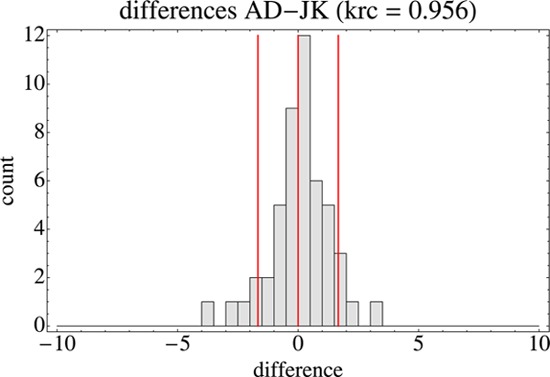
Histogram of rank differences for all points over all sessions for the observers AD and JK. The red lines indicate the ten and ninety percent quantiles and the median.

The differences are perhaps not entirely random, the major differences being concentrated on specific parts of the foreground and middle ground. This is typical for the other comparisons. It suggests that these are manifestations of idiosyncrasies of the observers. The data do not admit a precise analysis of this, though.

A matrix of Kendall rank correlations of the average rankings of all pairs of observers is shown in Table 1. All values are high; they range from 0.909 to 0.971. Apparently, all observers experience similar depth structures.

Table 1.

The Kendall rank correlations of the average rankings of all pairs of observers.

There are two independent measures that capture the depth resolution. One is the number of distinguished depth layers as obtained from the votes in single sessions. This turns out to be very similar across observers. The median number of resolved depth layers is 38, with an interquartile range of 4. Another measure is the ranking resolving power as determined from the scatter encountered in repeated sessions. It is defined as the number of points times one minus the mean Kendall rank correlation between rankings from different sessions. Its median value is 0.763, with an interquartile range of 0.403. The two measures are hardly correlated (coefficient of variation 0.034), mainly because neither varies much among observers. In Figure 11 we compare the number of distinguished depth layers between observers. There is hardly any variation. A similar conclusion results from a comparison of the ranking resolving power.

Figure 11.

At left, the number of distinguished depth layers for all observers. At right, the resolution in terms of ranking resolving power. The drawn line indicates the median, the gray area the interquartile range.

4.4. Correlation with metrical data from a previous experiment

In a previous experiment with a projective pointing method (Wagemans et al 2011), we determined metrical depth ranges for the same picture and the same observers as in the present experiment. This allows us to make an interesting comparison: Does the resolving power as determined from the present experiment co-vary with the metrical depth range? The comparison is an interesting one because the metrical depth ranges differ quite substantially between observers. Following Fechner's (1860) intuition, one might expect the depth range to be proportional to the number of resolved depth layers.

Firstly, we checked the Kendall rank correlation between the results of the two experiments. It turns out to be substantial. For 19 sessions by 6 observers (AD did 4 sessions, the others 3) we find 13 cases of perfect correlation, 1 case of 0.95, and 5 cases of rank correlation 0.8. Apparently, the observers report on very similar depth structures through the two very different operational methods.

As illustrated in Figure 12, we find nothing like the Fechner-type expectation. The resolving power as determined from the rank order appears essentially uncorrelated to the metrical depth range, irrespective of which measure is used.

Figure 12.

Left, the scatterplot of the number of resolved depth layers against the depth range from the pointing experiment for all observers. The coefficient of variation (R2) is 0.051. Right, the scatterplot of the ranking resolving power against the depth range from the pointing experiment for all observers. The coefficient of variation (R2) is 0.079.

This result is quite remarkable. Apparently, the observers are not really that different with regard to their depth-resolving power, even though they differ substantially with respect to their metrical depth ranges.

5. Discussion

We find only minor inter-observer differences, indicating that all observers experience very similar depth structures. The differences between any given pair of observers appear to be systematic rather than random, though. Apparently, there exist systematic, idiosyncratic differences, even though these are minor. We have not considered these in detail in this study. In order to do so, one would need to restructure the experiment in an appropriate way.

We find that the observers distinguished about 38 levels of the 49 point set and had a typical standard deviation of about one-and-a-half level. This indicates that the cardinality of the point set used here was perhaps marginal with respect to our aims. In order to draw conclusions and to be able to compare observers, we desire a broad spectrum of obvious errors. However, the scatter in the data turns out to be at least sufficient to enable us to draw some important conclusions.

An hour, or perhaps a little more, depending upon the observer, is about the maximum time span over which an observer is able to respond without detectable changes in “mental set.” In such a time one may collect about a thousand responses, limiting the cardinality of the point set to about 50. Thus, due to this time limit, it is not practical to use larger point sets with the method of pairwise comparison. We believe that the method as implemented by us is already close to the optimum that might be obtained by any method (eg, touch-screen implementation).

6. Conclusions

We designed, implemented, and thoroughly evaluated a simple method that allows one to find the depth rank order of up to 50 locations in a picture that is unlike a photographic rendering of a real scene, such as an imaginary landscape drawing or painting. The points need not be located on a single integral surface as is the case with a number of alternative depth probing methods we have investigated in the past (Koenderink and van Doorn 1995; Koenderink et al 2001; Koenderink and van Doorn 2003).

This is one method from a number of related methods that we have designed (and still are in the process of designing) to probe the geometrical structure of dispersed point sets in pictorial space (Wagemans et al 2011; van Doorn et al 2011; Koenderink and van Doorn 2003). No single method can reveal “the” depth structure; each method is one particular operationalization of “depth” (Koenderink et al 2011). It is only the comparison of several (as many as possible) methods that lets one approach the topic in a “method independent” way. Once such methods are in place, there are numerous interesting issues that can be addressed. We have already done so with the tools at our disposal (for example, oblique viewing, see Koenderink et al 2004; Wagemans et al 2011). The present method increases the scope.

We find that the observers (about half of them naive with respect to the experiment, all of them performing the task for the first time) yield very similar depth structures, with only very minor, though systematic, idiosyncratic variations. They resolve about 38 depth layers in a single session, with an uncertainty of about one-and-a-half level in repeated sessions.

It may be concluded that the method is entirely practical and yields useful results for the case of drawings and paintings. We believe it to be an excellent tool to probe the structure of pictorial depth for naive observers. This is expected to be useful in the study of pictorial cues, and the dependence of depth structure on “style,” for instance, depth in depictions from diverse cultures. This successfully concludes a major aim of this research, namely the implementation of a method to probe the depth structure of mutually dispersed points—not on a common surface—in pictorial space.

An important conclusion from these results is that the notion of a “pictorial space” has great utility, since it allows one to account for more than a thousand independent observations in terms of a rank order of about 50 items. Thus, pictorial space may be said to “exist” in this operational sense. This is of considerable interest because the term “pictorial space” is most often used as an essentially subjective notion, roughly as an indication of a person's visual awareness when looking “into” a picture.

Pictorial space has even greater utility because it has—in the above sense—been shown to exist relative to other, very different, operationalizations. In this study we have shown that the pictorial spaces obtained from the present ranking method, and a metrical pointing method (Wagemans et al 2011), are highly correlated. This greatly amplifies the utility of the concept. Apparently, pictorial space may be said to “exist” more or less independently of the method of operationalization. In future work we intend to increase the number of distinct operationalizations in order to check to what extent this conclusion holds up. It is a very important conceptual issue.

A possible application of our programme to build an extensive toolbox of essentially different methods that address nominally “the same” entity in pictorial space (such as depth) is to apply these to series of artworks taken from diverse periods or cultures. Since the various methods most likely put different weights on the various pictorial cues, one expects a different spectrum of results for the various cases. We already possess pilot data that reveal significant differences between depictions based on central perspective, and depictions that do not.

Although we indeed find a very high rank correlation of depths obtained by the two operationalizations mentioned above, we have encountered the lack of another relation that might well be expected on a priori grounds. This relation is the one originally proposed by Fechner (1860), namely that subjective magnitude scales should be “explained” through the discrimination thresholds. Fechner famously counted the number of just noticeable differences from the absolute threshold in order to arrive at a function that would be proportional to the subjective magnitude. In terms of the present experiment one might expect the total depth range found in the metrical operationalization to be inversely proportional to the resolved depth slice width as obtained from the pairwise rankings. We failed to confirm such a relation, however. Observers with rather different depth ranges still have very similar depth resolutions, thus Fechner's proposal fails completely for the depth domain.

A formal investigation of the properties of pictorial space suggests that the depth dimension is ambiguous in the sense that arbitrary contractions or dilations of the depth scale are consistent with all monocular pictorial cues (Koenderink and van Doorn 2008). This was already noticed intuitively by the German sculptor Hildebrand at the close of the 19th century (Hildebrand 1901). Thus, one expects the extent of the depth range in a pictorial space to be essentially idiosyncratic, or due to the “beholder's share” (Gombrich 1960). We have indeed found this in former experiments (Koenderink et al 1994; Koenderink et al 2001; Koenderink and van Doorn 2003). The differences between observers may be as large as a factor of four (Koenderink et al 1994). In view of this, the failure of Fechner's relation need perhaps not be too surprising. It is the result of the fact that the depth calibration is essentially “mental paint,” that is to say, cannot be based on the monocular cues. That this ambiguity is not encountered in the present experiment is due to the method, namely that we determine a depth ranking order, not a metrical order.

Biography

Jan Koenderink (1943) studied physics, mathematics, and astronomy at Utrecht University, where he graduated in 1972. From the late 1970's he held a chair “The Physics of Man” at Utrecht University till his retirement in 2008. He presently is Research Fellow at Delft University of Technology and guest professor at the University of Leuven. He is a member of the Dutch Royal Society of Arts and Sciences and received a honorific doctorate in medicine from Leuven University. Current interests include the mathematics and psychophysics of space and form in vision, including applications in art and design.

Andrea van Doorn (1948) studied physics, mathematics, and chemistry at Utrecht University, where she did her master's in 1971. She did her PhD (at Utrecht) in 1984. She is presently at Delft University of Technology, department of Industrial Design. Current research interests are various topics in vision, communication by gestures, and soundscapes.

Johan Wagemans (1963) has a BA in psychology and philosophy, an MSc and a PhD in experimental psychology, all from the University of Leuven, where he is currently a full professor. Current research interests are mainly in so-called mid-level vision (perceptual grouping, figure-ground organization, depth and shape perception) but stretching out to low-level vision (contrast detection and discrimination) and high-level vision (object recognition and categorization), including applications in autism, arts, and sports (see http://www.gestaltrevision.be)

Appendix: The ranking algorithm

This appendix motivates our choice of ranking algorithm. We used a voting procedure, whereas most of the literature uses one of the conventional procedures that are guaranteed to yield an approximation to the “best” solution in some formal sense. The essential difference lies in the fact that we use a full data set, whereas one typically uses rather less than that. The reason is obvious enough, namely that the number of pairwise judgments for a full data set grows like the square of the number of items. Thus, practical limits on the session length in most cases render it impossible to collect a full data set. For our kind of problem this is not out of the question, though; for 50 items (say) one needs to run 1,225 trials, so a full session can still be completed in an hour when the response time is less than 3 s.

The analysis of a full data set is different (much easier, but also different in kind) from what applies to an incomplete one. Here we discuss the major points of concern.

This appendix is necessarily of a technical nature, but we make every attempt to keep it simple and yet make the essential issues conceptually clear. In order to achieve this, we use a small “toy” example. Any such example has to be small, because the complexity of the problem grows exponentially with the number of items. Only for sufficiently small examples can one illustrate everything explicitly. Here we use a set of only 7 items. (We have been able to confirm our conclusions for sets of up to 12 items; larger sets require supercomputers or very long time spans.) Notice that this implies that there are already 5,040 distinct rankings. A full session implies 21 pairwise comparisons, on the basis of which one attempts to select the “best” (in some sense) possible ranking out of these 5,040.

First, we illustrate the basic voting procedure. Take seven items with known values one to seven. Suppose the pairwise rankings are perfect, for instance, the comparison of item three (value three) with item six (value six) will yield the result that item six is larger than item three (because six exceeds three). Thus, the matrix of responses will be:

	1	2	3	4	5	6	7
1	∗	+	+	+	+	+	+
2	−	∗	+	+	+	+	+
3	−	−	∗	+	+	+	+
4	−	−	−	∗	+	+	+
5	−	−	−	−	∗	+	+
6	−	−	−	−	−	∗	+
7	−	−	−	−	−	−	∗

Here a plus-sign means “larger than,” a minus-sign means “smaller than,” and an asterisk-sign means that the combination was never presented. Notice that the half of the matrix beneath the diagonal can be ignored, too, because all combinations were presented only once; thus the results can be collected in the half above the diagonal. (One may move an item from below to above the diagonal by inverting it.) Now we count “larger than votes,” that is the number of plus signs. We find zero, one, two, three, four, five, and six votes for the items one, two, three, four, five, six, and seven, respectively. Thus, the number of votes plus one perfectly recovers the correct ranking. This is the essential idea. Finding the ranking is implemented through computing row (or column) sums in the data matrix. The reader who is only interested in a practical algorithm may stop reading here. Notice that the algorithm is fast and easy to implement.

In this ideal toy example we had “ground truth” at our disposal, and we simulated perfect data. In real life one has neither. One may still apply the voting method, but it is less immediately obvious what the result may mean.

In order to make the example more realistic, we draw the values from a random distribution on the range 0 to 100. We sort the values, so the items are still in correct rank order. This is not necessary, but it largely simplifies the presentation of the example. Doing the same experiment as above will evidently yield the same result. In order to make the example more realistic, one needs to introduce a degree of uncertainty. We do this by two simple operations:

• Firstly, we add a dither to the values. For the example we add normally distributed deviations of standard deviation two times the range (100) divided by the number of points (7), thus 28.57…. This simulates the intrinsic uncertainty of the observer. Given these perturbed values, we may find the answers to all pairwise judgments.

• Secondly, we randomly swap 5% of the answers, here just one of these. This simulates mistakes such as hitting the wrong button, which are almost certain to occur in any psychophysical session of an hour or so.

Thus, we end up with a response matrix that will be different from the ideal one shown above. In one particular run, that will be used as an example here, we found:

	1	2	3	4	5	6	7
1	∗	+	+	+	+	+	+
2	−	∗	−	+	+	+	+
3	−	+	∗	+	+	+	+
4	−	−	−	∗	−	+	+
5	−	−	−	+	∗	−	+
6	−	−	−	−	+	∗	+
7	−	−	−	−	−	−	∗

Using the same voting procedure, we end up with some ranking order that will be referred to as the “voting order.”

The voting order will typically differ from the ground truth. It is also typically incomplete, in the sense that several items may receive an equal number of votes. Thus, there will be “ties.” For instance, in the example run we counted the votes (1,3,2,5,5,5,7), which differs from the ground truth (1,2,3,4,5,6,7) in that items two and three appear in the reverse order, whereas items four, five, and six yield a tie. Notice that orders four and six do not occur. This is not even a bad result, though, since the Kendall rank correlation with the ground truth is 0.823.

We define the “figure of merit” (FOM) of a ranking as a measure of the degree to which that ranking accounts for the pairwise judgments. The FOM is defined much like the familiar Kendall rank order correlation (Kendall 1955), namely as the number of explained pairwise orders minus the number of not explained pairwise orders divided by the total number of pairs. Thus, the FOM ranges between minus and plus one; in practice, it is typically a number close to but less than one.

The figure of merit of the voting order is 0.857. It comes perhaps as a surprise that the figure of merit of the ground truth is lower than that, namely 0.714. This happens because the perturbed values are actually in a different order than the ground truth, whereas the voting method tries hard to estimate these perturbed values. In that sense the “figure of merit” is meaningless. It is useful in the context of this example though, where we actually have ground truth at our disposal.

From a conceptual point of view one may define the “best” ranking order as the one that accounts for most of the pairwise judgments (highest FOM). There exist algorithms that approximately find one or more of the best solutions, or at least close approximations to these, even in cases of an incomplete data matrix (Bradley and Terry 1952; Remage and Thompson 1966; deCani 1969). For the case of the toy example such a best ranking order may be discovered simply by going through all of the 5,040 possible rank orders. We find that such best orders are not necessarily unique. In a run of 500 we found 61 unique best rankings, the highest multiplicity being nine (encountered two times).

Since such rankings are equally good, there is no way to choose between them. For the example run we found three “best” rankings, namely (1,3,2,4,6,5,7), (1,3,2,5,4,6,7), and (1,3,2,6,5,4,7), which each have a figure of merit of 0.905. This value (being the best) is, of course, higher than that for the voting order, but the fact that the voting order scores better than the ground truth is some reason to doubt the relative importance of these values. The Kendall rank correlations of the best ranking orders with the ground truth are 0.810, 0.810, and 0.619. Thus, the voting order correlates better with the ground truth than the best orders, whereas the best orders differ greatly among themselves in this respect.

If one perturbs an order by swapping pairs of neighbours, one obtains a set of slightly different orders. The “robustness” of an order may be probed by finding the range of Kendall rank correlations for such a set of perturbed orders. For the example the range for the voting order is 0.720 to 0.926, whereas the total range for the “best” orders, taken together, is 0.524 to 0.905. (Notice that the quality of the voting order may increase through a perturbation, whereas that of a best order can only decrease.) The lowest best order (0.619) lies below the range for the voting order, whereas the highest best order (0.810) is included in it. Apparently, one might do worse than by adopting the voting order in preference to a best order. The reason is, of course, that the notion of “best” ignores the fact that one desires to approximate the ground truth, but actually attempts to account for the data as well as possible.

From such examples one gleans that methods that attempt to find the order(s) that best account for the data are not necessarily to be preferred. It would be preferable to use a method that on the average approaches the ground truth, with little spread. In a large simulation we find that the voting order is always equal or better than the median of the “best” orders in terms of rank correlation with the ground truth. The range of rank correlations for the “best” orders is large and includes instances that are far from the ground truth. Usually one encounters a number of best orders that are much worse than the voting order. Thus, the voting method yields much more robust results. In cases of low levels of perturbation the voting order is almost the same as any of the best orders (which differ little among themselves). It may be concluded that one is better off with the (very simple!) voting order than with an arbitrary member of the best orders. (Note that there is no criterion by which to pick the most desirable best order in the absence of ground truth.)

One may attempt to improve on the simple voting method, using the procedure of “runoff voting” (Slater 1961; Tullock 1964). One selects the candidates for which a tie was found and considers the votes cast on this subset. That this is likely to refine the result is evident when one considers the case of a tie between a pair of candidates. Because the pair was actually compared in some trial, the rank order for any pair considered as a pair is well defined! The tie was caused by the comparisons of each of the two candidates with all the others. Runoff voting can of course be applied to ties of any cardinality. One simply applies the voting procedure in an iterative fashion. The resolved ties may contain ties of a higher order which may perhaps be resolved through another application of runoff voting, and so forth. It is not guaranteed that one arrives at a fully resolved ranking order though. The resulting ties are due to “intransitive sets” that allow of no further resolution. In the above example the items four, five, and six form such an intransitive set; thus iterative runoff voting does not serve to refine the example. In many cases it does, though. There is no alternative but to assign equal rank to the members of an intransitive set (typically triplet).

The number of triplets grows with the cube of the number of items. In the example there exist 35 triangles, apparently one of these intransitive. The intransitive triangles may be found by exhaustive search in this small example; in larger problems this is usually out of the question. For 50 items one has already 19,600 triangles.

The iterative runoff voting implements a Condorcet voting method (Rousseau 1984; Condorcet 1785; Young and Levenglick 1978; Grofman and Feld 1988; Young 1988). A “Condorcet winner” is the person who would win a two-candidate election against each of the other candidates, if such a candidate exists. Typically, such a candidate will not exist, a fact known as “Condorcet's paradox,” forcing one to fall back on some approximation as the one presented here.

To put things into proper perspective, in virtually all cases the simple voting already produces an excellent result that is hardly changed much through the procedure of iterative runoff voting. In fact, the results presented in this paper would look much the same had we omitted this refinement.

References

- Berkeley G. An Essay Towards a New Theory of Vision. Dublin, UK: Aaron Rhames; 1709. [Google Scholar]
- Bradley R A, Terry M E. “Rank analysis of incomplete block designs: I. The method of paired comparisons”. Biometrika. 1952;39:324–345. [Google Scholar]
- Cohn J. “Experimentelle Untersuchungen über die Gefühlsbetoningen der Farben, Helligkeiten und ihrer Combinationen”. Philosophische Studien. 1894;10:562–603. [Google Scholar]
- Condorcet J-A-N. Essai sur l'application de l'analyse à la probabilité des décisions rendues à la pluralité des voix. Paris, France: De l'Imprimerie Royale; 1785. [Google Scholar]
- Cott H B. Adaptive Coloration in Animals. London: Methuen; 1957. [Google Scholar]
- deCani J S. “Maximum likelihood paired comparison ranking by linear programming”. Biometrika. 1969;56:537–545. doi: 10.1093/biomet/56.3.537. [DOI] [Google Scholar]
- Denis M. Art and the Academy in the Nineteenth Century. Piscataway, NJ: Rutgers University Press; 2000. “Manifesto of the style nabi: Definition of neo-traditionalism [Définition du néo-traditionnisme in Art et Critique (1890)]”. [Google Scholar]
- Fagot L. Picture Perception in Animals. London: Psychology Press; 2001. [Google Scholar]
- Fechner G T. Elemente der Psychophysik II. Leipzig, Germany: Thoemmes Press; 1860. [Google Scholar]
- Gibson J J. The Perception of the Visual World. Boston, MA: Houghton Mifflin; 1950. [Google Scholar]
- Gombrich E H. Art and Illusion. A Study of the Psychology of Pictorial Representation. London: Phaidon Press; 1960. [Google Scholar]
- Grofman B, Feld S L. “Rousseau's general will: A Condorcetian perspective”. The American Political Science Review. 1988;82:567–576. doi: 10.2307/1957401. [DOI] [Google Scholar]
- Hildebrand A. Das Problem der Form in der bildenden Kunst. Strassburg, France: Heitz & Mündel; 1901. [Google Scholar]
- Ittelson W H. The Ames Demonstrations in Perception. Princeton, NJ: Princeton University Press; 1952. [Google Scholar]
- Kemeny J G. “Mathematics without numbers”. Daedalus. 1959;88:577–591. [Google Scholar]
- Kendall M G. Rank Correlation Methods. New York: Hafner Publishing Co; 1955. [Google Scholar]
- Kendall M G, Babington-Smith B. “On the method of paired comparisons”. Biometrika. 1940;31:324–324. [Google Scholar]
- Koenderink J J, van Doorn A J. “Relief: Pictorial and otherwise”. Image and Vision Computing. 1995;13:321–334. doi: 10.1016/0262-8856(95)99719-H. [DOI] [Google Scholar]
- Koenderink J J, van Doorn A J. “Pictorial space” Looking into Pictures: An Interdisciplinary Approach to Pictorial Space. Cambridge, MA: MIT Press; 2003. [Google Scholar]
- Koenderink J J, van Doorn A J. “The structure of visual spaces”. Journal of Mathematical Imaging and Vision. 2008;31:171–187. doi: 10.1007/s10851-008-0076-3. [DOI] [Google Scholar]
- Koenderink J J, van Doorn A J, Kappers A M L. “On so-called paradoxical monocular stereoscopy”. Perception. 1994;23:583–594. doi: 10.1068/p230583. [DOI] [PubMed] [Google Scholar]
- Koenderink J J, van Doorn A J, Kappers A M L. “Pictorial surface attitude and local depth comparisons”. Perception & Psychophysics. 1996;58:163–173. doi: 10.3758/BF03211873. [DOI] [PubMed] [Google Scholar]
- Koenderink J J, van Doorn A J, Kappers A M L, Todd J T. “Ambiguity and the ‘mental eye’ in pictorial relief”. Perception. 2001;30:431–448. doi: 10.1068/p3030. [DOI] [PubMed] [Google Scholar]
- Koenderink J J, van Doorn A J, Kappers A M L, Todd J T. “Pointing out of the picture”. Perception. 2004;33:513–530. doi: 10.1068/p3454. [DOI] [PubMed] [Google Scholar]
- Koenderink J J, van Doorn A J, Wagemans J. “Depth”. i-Perception. 2011;2:541–564. doi: 10.1068/i0438aap. [DOI] [PMC free article] [PubMed] [Google Scholar]
- Luce R D. Individual Choice Behavior: A Theoretical Analysis. New York: Wiley; 1959. [Google Scholar]
- Pirenne M H. Optics, Painting and Photography. Cambridge, MA: Cambridge University Press; 1970. [Google Scholar]
- Remage R, Thompson W A. “Maximum-likelihood paired comparison rankings”. Biometrika. 1966;53:143–149. [PubMed] [Google Scholar]
- Rousseau J J. Of the Social Contract, or Principles of Political Right & Discourse on Political Economy [Du contrat social ou Principes du droit politique (1762)] New York: Harper & Row; 1984. [Google Scholar]
- Schwartz T. “Rationality and the myth of the maximum”. NoÛs. 1972;6:97–117. [Google Scholar]
- Slater P. “Inconsistencies in a schedule of paired comparisons”. Biometrika. 1961;48:303–312. [Google Scholar]
- Thurstone L L. “A law of comparative judgment”. Psychological Review. 1927;34:273–286. doi: 10.1037/h0070288. [DOI] [Google Scholar]
- Thurstone L L. “The measurement of psychological value” Essays in Philosophy by Seventeen Doctors of Philosophy of the University of Chicago. Chicago, IL: Open Court; 1929. [Google Scholar]
- Thurstone L L. The Measurement of Values. Chicago, IL: The University of Chicago Press; 1959. [Google Scholar]
- Titchener E B. Experimental Psychology: I. Qualitative Experiments. London: MacMillan and Co Ltd; 1901. [Google Scholar]
- Titchener E B. Lectures on the Elementary Psychology of Feeling and Attention. New York: The Macmillan Company; 1908. [DOI] [Google Scholar]
- Tullock G. “The irrationality of intransitivity”. Oxford Economic Papers. 1964;16:401–406. [Google Scholar]
- van Doorn A J, Wagemans J, de Ridder H, Koenderink J J. “Space perception in pictures”. Proceedings of SPIE. 2011;7865:786519–786519. doi: 10.1117/12.882076. [DOI] [Google Scholar]
- Wagemans J, van Doorn A J, Koenderink J J. “Measuring 3D point configurations in pictorial space”. i-Perception. 2011;2:77–111. doi: 10.1068/i0420. [DOI] [PMC free article] [PubMed] [Google Scholar]
- Wickler W. Mimicry in Plants and Animals. New York: McGraw-Hill; 1968. [Google Scholar]
- Wittgenstein L. “Logisch-Philosophische Abhandlung”. Annalen der Naturphilosophie. 1921:14. [Google Scholar]
- Wittmer L. “Zur experimentellen Ästhetick einfacher räumliche Formverhältnisse”. Philosophische Studien. 1894;9:96–144. 209–263. [Google Scholar]
- Young H P. “Condorcet's theory of voting”. The American Political Science Review. 1988;82:1231–1244. doi: 10.2307/1961757. [DOI] [Google Scholar]
- Young H P, Levenglick A. “A consistent extention of Condorcet's election principle”. SIAM Journal on Applied Mathematics. 1978;35:285–300. doi: 10.1137/0135023. [DOI] [Google Scholar]