Automatic Detection of Tree-in-Bud Patterns for Computer Assisted Diagnosis of Respiratory Tract Infections

Abstract

Abnormal nodular branching opacities at the lung periphery in Chest Computed Tomography (CT) are termed by radiology literature as tree-in-bud (TIB) opacities. These subtle opacity differences represent pulmonary disease in the small airways such as infectious or inflammatory bronchiolitis. Precisely quantifying the detection and measurement of TIB abnormality using computer assisted detection (CAD) would assist clinical and research investigation of this pathology commonly seen in pulmonary infections. This paper presents a novel method for automatically detecting TIB patterns based on fast localization of candidates using local scale information of the images. The proposed method combines shape index, local gradient statistics, and steerable wavelet features to automatically identify TIB patterns. Experimental results using 39 viral bronchiolitis human para-influenza (HPIV) CTs and 21 normal lung CTs achieved an overall accuracy of 89.95%.

I. INTRODUCTION

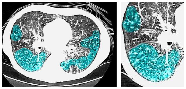
A common pattern of abnormality on Chest CT is TIB opacity, in which thickened peripheral lung structures have adjacent clusters of nodules, and generally represent disease of the small airways (bronchioles) such as infectious or inflammatory bronchiolitis [1]. TIB on Chest CT indicates bronchiolar luminal impaction with mucus, pus, cells or fluid causing normally invisible peripheral airways to become visible [1], as shown in Figure 1. The precise quantification of lung volume affected by this disease process has been limited by inter-observer variance with inconsistent visual scoring methods. A CAD system designed to detect and quantify TIB would add precision to the analysis of infectious lung disease. However, there are many difficulties in detecting TIB opacities. First, micro-nodules and abnormal peripheral airway structures have strong shape and appearance similarities to normal anatomical structures in the lungs. Second, TIB often appears as a mixture of normal and abnormal patterns because of the close anatomical proximity of normal and abnormal regions, hence, discriminating those patterns is often challenging.

Fig. 1.

(Left) CT image with a significant amount TIB patterns. TIB patterns are labelled in blue. (Right) Zoomed window on the right lung.

In this study, we propose a new CAD system to quantify pulmonary infections by automatically detecting TIB patterns. The contributions of the paper are two-fold: (1) Based on texture and shape characteristics of TIB patterns, a candidate selection method is proposed. (2) We propose to use an integrated feature extraction scheme combining local shape features, local gradient statistics, and steerable features to specify TIB patterns. By candidate selection method, all possible abnormal patterns are localized in the lung fields. Next, we define local regions enclosing each candidate pattern and extract shape and texture features from local regions. Extracted features are classified as TIB or normal using support vector machines (SVM). We compare our proposed CAD system on the basis of different feature sets previously shown to be successful in detecting lung diseases in general.

II. CAD Algorithm

The proposed CAD system is illustrated in Figure 2. First, lungs are segmented from CT volumes. Second, locally adaptive scale based filtering is used to identify candidate TIB pattern regions. Third, a local window is used around each candidate point to define some discriminatory intrinsic shape and textural features followed by SVM classification. The results of the pixel-wise classification are presented as area under receiver operating characteristic (ROC) curves (A_z).

Fig. 2.

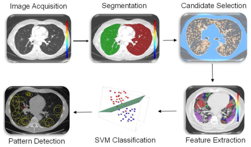
The flowchart of the proposed TIB detection system.

A. Segmentation

Segmentation is often the first step in typical CAD systems. In this study, fuzzy connectedness (FC) image segmentation algorithm [2] is used. In this study, to initiate FC segmentation, two seeds per volume (i.e., one for the right lung and one for the left lung) are selected automatically by only considering the locations of small intensity valued pixels inside the body region.

B. Candidate Selection

TIB patterns have intensity characteristics having high variation towards nearby pixels. The size of the body of a TIB pattern and micro-structures nearby the body of the TIB pattern do not exceed a few pixels in length. This implies that TIB patterns are localized only in the vicinity of small scale regions. In other words, TIB patterns do not constitute sufficiently homogeneous regions over large regions. Non-smooth changes in local gradient values support this observation. As guided by these observations, we propose to use a locally adaptive scale filtering to identify small scale regions. Those small scale regions are named candidate regions. Selecting candidate regions do not only restrict the problem into a smaller subspace but also decrease the computational time due to avoiding elaborate search on the large homogeneous regions in the images.

As opposed to well known multi-scale global approaches [3], we use the concept of “scale” in the locally adaptive sense [2]. In this phenomenon, the size of the scale is allowed to change in different parts of the image. Based on continuity of homogeneous regions, geometric properties of objects (i.e., scale information) can be identified. In this study, we define candidate TIB regions with ball-scale (or b-scale for short) filtering followed by thresholding [5]. The details of this process are explained in the next subsection.

1) Ball Scale Encoding

The main idea in b-scale encoding is to determine the size of local structures at every pixel as the radius of the largest ball centered at the pixel within which intensities are homogeneous under a pre-specified region-homogeneity criterion. In this paper, we use 2-dimensional b-scale encoding due to the following fact: TIB patterns are small anatomical structures as seen in Figure 1 that in order to fully appreciate their anatomical details, thin slice CT scans with sub-millimeter resolution (high resolution CT) are necessary. However, the CT data at hand is low resolution with 5 mm slice spacing, which do not allow continuous analysis of TIB patterns through low resolution imaging direction.

In the 2D digital space (Z², v), a scene = (C,f) is represented by a pair where C is a rectangular array of pixels, v = (v₁, v₂) indicates the size of the pixels, and f is a function that assigns to every pixel an image intensity value. A ball B_k,v(c) of radius k ≥ 0 and with center at a pixel c ∈ C in is defined by

$${\text{B}}_{\text{k},\text{v}}(\text{c})=\left\{\text{e}\in \text{C}|\sqrt{\sum _{\text{i}=1}^{\text{n}}\frac{{\text{v}}_{\text{i}}^2{({\text{c}}_{\text{i}}-{\text{e}}_{\text{i}})}^2}{{min}_{\text{j}}\left[{\text{v}}_{\text{j}}^2\right]}}\le \text{k}\right\}.$$ (1)

The fraction of object is denoted by FO_k,v(c) and indicates the fraction of the ball boundary occupied by a region which is sufficiently homogeneous with c. FO_k,v(c) is defined as

$${\text{FO}}_{\text{k},\text{v}}(\text{c})=\frac{{\sum }_{\text{e}\in {\text{B}}_{\text{k},\text{v}}(\text{c})-{\text{B}}_{\text{k}-1,\text{v}}(\text{c})}{\text{W}}_{\psi }(\mid \text{f}(\text{c})-\text{f}(\text{e})\mid )}{\mid {\text{B}}_{\text{k},\text{v}}(\text{c})-{\text{B}}_{\text{k}-1,\text{v}}(\text{c})\mid }$$ (2)

where |B_k,v(c) − B_k−1,v(c)| is the number of pixels in B_k,v(c)−B_k−1,v(c) and W_ψ is a homogeneity function [2]. In all experiments, we use a zero-mean un-normalized Gaussian function for W_ψ. As it is readily seen that the size of a local structure is estimated using appearance information of the grey level images, i.e., region-homogeneity criterion, b-scale scenes contain rough geometric information. A detailed description of W_ψ and FO_k,v are presented in [2].

2) Candidate Identification via Scale Selection

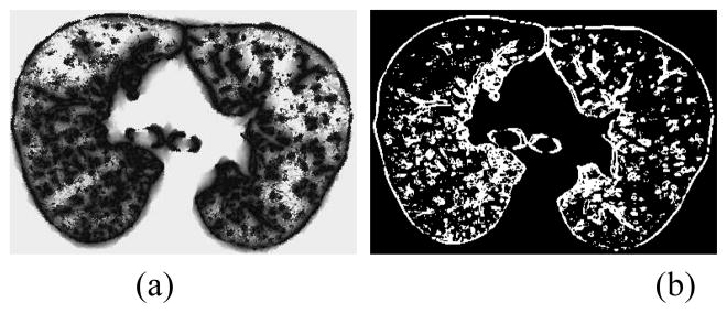
In principle, b-scale partitions the scene into several levels based on the size of local structures. Note that locally adaptive scale in regions with fine details or in the vicinity of boundaries is small, while it is large in the interior of a large homogeneous objects. Since it is observed that TIB patterns constitute only small b-scale values, it is highly reasonable to consider pixels with small b-scale values as candidate TIB patterns, and discard pixels with high b-scale values. Figure 3 shows a b-scale scene (a) and b-scale scenes with selected scales (i.e., smallest scales) (b). This selection process, namely selecting only smallest scales from b-scale image, does not only guarantee choosing areas with TIB patterns as candidate regions, but as its simplest, it allows elimination of large homogeneous objects from candidate selection procedure.

Fig. 3.

(a) b-scale scene. (b) Thresholded b-scale scene, pixels having only smallest b-scale values are selected as candidate TIB patterns.

III. Feature Extraction

TIB pattern has a complex shape structure, consisting of curvilinear structures around which nodular structures exist (i.e., a budding tree). In order to have sufficient discriminatory power to distinguish TIB patterns, there is a need to have representative features characterizing shape and texture of TIB patterns efficiently. To achieve this, we propose to use shape index and statistics over local gradients in different thresholds to obtain intrinsic shape descriptors for a given local window around each candidate pattern. In addition, we use steerable features to capture local appearance information. While shape features characterize the curvilinear structures (via shape index) and small nodular structures (via shape index and statistics over local gradients), steerable features characterize background and foreground intensity variation with objects’ pose and size for a given local window. These feature sets are described in the following subsections.

Shape Index (SI)

The shape index (SI) is a statistical measure and used to define intrinsic shape of the localized structure within the image [4]. SI values are encoded as a continuous range of values between −1 and 1, with zero SI indicates saddle-like local structures, +1 and −1 SI values indicate umbilical minima and maxima (i.e., cap and cup, respectively), and mid-points of the two half-intervals (+0.5 and −0.5) indicate concave and convex parabolic or line-like structures (i.e., rut and ridge, respectively). SI can simply be computed through principal curvatures (κ₁,κ₂) as follows:

$$\text{SI}=\frac{2}{\pi }arctan(\frac{{\kappa }_1+{\kappa }_2}{{\kappa }_1-{\kappa }_2})\in [-1,1]$$ (3)

where κ₁ and κ₂ are principal curvatures (κ₁ ≥ κ₂). As suggested in [4], we obtain principal curvatures from the eigenvalues of the local Hessian matrix (H) as:

$$\text{H}=\left(\begin{array}{cc}{\text{L}}_{\text{xx}}& {\text{L}}_{\text{xy}}\\ {\text{L}}_{\text{yx}}& {\text{L}}_{\text{yy}}\end{array}\right)$$ (4)

where L_xx,L_xy = L_yx, and L_yy are second order derivatives of local image patch ℒ.

Shape Statistics over Local Gradient (LGS)

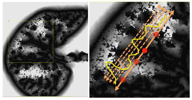
Gradient fields can be used effectively to obtain statistical measures for a given local window. For example, TIB patterns consist of numerous small (or micro-) nodules nearby the main curvilinear structure and those small structures have varying opacities. One may obtain the location and distribution of those small structures by simple thresholding which has been popular in estimation for more than two decades [6], however, since the opacities are varying through different nodular structures, it is challenging to find an optimum threshold value. Therefore, instead of using one single threshold level, we use n = 10 different threshold levels (λ_j) to obtain local statistics of those structures in a hierarchical way, where λ_j = 10j, 1 ≤ j ≤ 10 [9]. Figure 4 shows an example threshold selection process for four levels over a candidate TIB pattern centered at c. The number of b-scale patterns over the local region for each thresholding level and mean SI value over the local region for each different threshold level are recorded as discriminative features explaining intrinsic shape statistics. Although n and λ_j are chosen emprically based on the observations of shape and textural characteristics of normal and TIB patterns during the training, one may propose to use cross-validation, control of the global and local false discovery rate, and uncertainty principles to decide those parameters near-optimally [6].

Fig. 4.

Local gradient maxima above different thresholds are found.

Steerable Features

It has been well documented in the literature that decomposition of images by using basis functions localized in spatial position, orientation, and scale (e.g., wavelets) are extremely useful in object recognition and detection [7]. Since steerable filters are rotation and translation invariant, they accurately represent the underlying image structure [8]. In this study, we use steerable Derivative of Gaussian (DoG) filters to decompose local regions around each candidate into several oriented basis. These basis are used as features in pixel-wise classification for TIB identification. We extract steerable features (i.e., directional derivatives) from 1 scale and 6 different orientations. For a comparison, we also extract Grey-Level Co-occurrence Matrix (GLCM) based features [10], which are shown to be useful in discriminating and quantifying patterns pertaining to lung diseases. For each local patch, we extract 18 GLCM based features including autocorrelation, contrast, entropy, variance, dissimilarity, homogeneity, and extended features of those.

For a local region centered at a pixel c of a candidate TIB pattern, we extract 1 feature as a SI value of the pixel c, 3 features as the maximum, minimum, and mean SI values over the local region, 10 features as mean SI values (due to 10 thresholding level from statistics of local gradients), and 10 features as the number of selected (smallest) b-scale patterns over the local region, resulting in a total of 24 features (SI+LGS). Steerable wavelet feature extraction scheme leads to its features having the dimensions of 486, 1014, and 1734, if local window of sizes 9×9, 13×13, and 17×17 are used, respectively.

IV. Experimental Results

Laboratory confirmed 39 CTs of HPIV infection and 21 normal lung CTs were collected for the experiments. The in-plane resolution is affected from patients’ size and varying from 0.62mm to 0.82mm, and the slice thickness of the scans is 5mm. After data collection, an expert radiologist (DJM) carefully examined the complete scans and labeled the regions as normal or TIB opacity with the number of respective regions shown in Table I. Next, corresponding b-scale scenes are computed from labeled grey level CT images. Scale selection procedure is applied to the b-scale scenes, and all the pixels within the ground-truth (labeled regions) are used to extract features over local patches of size |ℒ| =9×9, 13×13, or 17×17. Those extracted features (labeled as normal and TIB) are then used to train SVM classifier. We use two-fold cross validations to make optimal use of available data.

TABLE I.

Number of local patches used in the experiments.

Patch Size ℒ	TIB	Normal
9×9	50456	42924
13×13	24184	20572
17×17	14144	12032

Evaluation of the CAD algorithm includes a performance measure of a computer output determined alone from appropriate detection/classification. Our observations show that only 21%–40% of the segmented lung volume is chosen as candidate TIB patterns. This interval is subject to change based on the severity of the diseases (i.e., more TIB patterns). For normal patients, for instance, the percentage of the candidate regions is smaller than the patients with infections (21% < 40%). Having said that, local scale might perhaps be used as a quantitative measure validating the sensitivity and specificity of the classification rates.

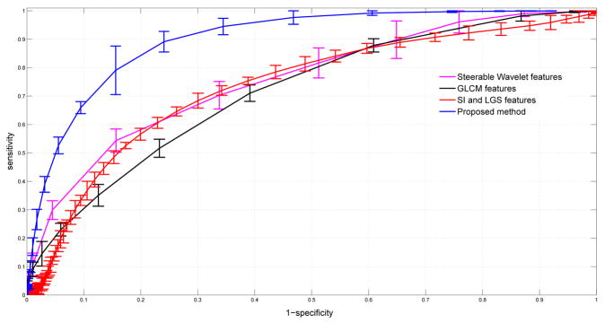
Table II shows the performance of the proposed CAD system as compared to other feature sets. The performances are reported as the areas under the ROC curves (A_z). Note that we also include SI & LGS features without combining with steerable wavelet features. Even being used alone, SI & LGS features show superior performance to other methods while the dimension of the feature set is only 24. The best performance is obtained with the proposed method which combine SI & LGS with steerable wavelet features. In what follows, we select the best window size for each feature set and plot their ROC curves all in Figure 5. To have a valid comparison, we repeat candidate selection step for all the methods, hence, the CAD performances of compared feature sets might perhaps have lower accuracies if the candidate selection part is not applied. To show whether the proposed method is significantly different than the other methods, we compared the performances through evaluation paired t-tests, and the p-values of the tests are summarized in Table III. Note that statistically significant changes are emphasized by in two different statistical levels, p < .05 and p < .01, respectively.

TABLE II.

Accuracy (A_z) of the CAD system with given feature sets.

Features	Dimension	Patch Size ℒ	Az
Proposed features	6 × 17×17 + 24=1760	17×17	0.8680
Proposed features	6×13×13 + 24=1038	13×13	0.8995*
Proposed features	6×9×9 + 24=510	9×9	0.8800
SI & LGS	24	17×17	0.7620
SI & LGS	24	13×13	0.7510
SI & LGS	24	9×9	0.7230
Steer. Wave.	6×17×17=1734	17×17	0.7571
Steer. Wave.	6×13×13=1014	13×13	0.7298
Steer. Wave.	6×9×9=486	9×9	0.7410
GLCM	18	17×17	0.7163
GLCM	18	13×13	0.7068
GLCM	18	9×9	0.6810

Fig. 5.

Comparison of CAD performances via ROC curves of different feature sets.

TABLE III.

p-values are shown in confusion matrix.

p-Confusion	SI& LGS	Steer. Wave.	GLCM
Proposed Method	<0.01	<0.01	<0.01
SI& LGS	–	<0.05	<0.01
Steer. Wave.	–	–	<0.01

V. Conclusion

In this paper, we have proposed b-scale based binary classification approach for automatic TIB pattern detection from lung CTs. The proposed system integrates 1) fast localization of candidate TIB patterns through b-scale filtering and scale selection, and 2) combined shape and textural features to identify TIB patterns. Experimental results using 39 laboratory confirmed viral bronchiolitis (parainfluenza) CTs and 21 normal lung CTs achieved the performance of A_z=0.8995. To further eliminate the false positive fraction, one may train boosting classifiers to select strong features rather than rare and weak features prior to SVM classification. As a future extension of this study, one may consider using a feature selection method to explore the effect of local window size and optimal feature selection. In this paper, we have not addressed the issue of quantitative evaluation of severity of diseases by expert observers. This is a challenging task for complex shape patterns such as TIB opacities, and subject to further investigation.

References

- 1.Eisenhuber E. The tree-in-bud sign. Radiology. 2002;222(3):771–772. doi: 10.1148/radiol.2223991980. [DOI] [PubMed] [Google Scholar]
- 2.Saha PK, et al. Scale-based fuzzy connected image segmentation: Theory, algorithms, and validation. Computer Vision Image Understanding. 2000;77:145–174. [Google Scholar]
- 3.Tabb M, Ahuja N. Multiscale image segmentation by integrated edge and region detection. IEEE Transactions on Image Processing. 1997;6(5):642–655. doi: 10.1109/83.568922. [DOI] [PubMed] [Google Scholar]
- 4.Koenderink JJ, van Doorn AJ. Surface shape and curvature scales. Image Vision and Computing. 1992;10(8):557–565. [Google Scholar]
- 5.Bagci U, Udupa JK, Chen X. Ball-Scale Based Multi-Object Recognition in a Hierarchical Framework. Proc of SPIE Medical Imaging. 2010;7623(762345):1–12. [Google Scholar]
- 6.Donoho D, Johnstone I. Minimax risk Ip-balls for Iq-error. Probab Theory Relat Fields. 1994;2:277–303. [Google Scholar]
- 7.Bagci U, Li B. Parallel AdaBoost Algorithm for Gabor Wavelet Selection in Face Recognition. Proc of IEEE ICIP. 2008:1640–1643. [Google Scholar]
- 8.Freeman T, Adelson EH. The design and use of steerable filters. IEEE Transactions on Pattern Analysis and Machine Intelligence. 1991;13(9):891–906. [Google Scholar]
- 9.Barbu A, et al. Automatic Detection and Segmentation of Axillary Lymph Nodes. Proc of MICCAI. 2010:28–36. doi: 10.1007/978-3-642-15705-9_4. [DOI] [PubMed] [Google Scholar]
- 10.Haralick RM, et al. Textural Features for Image Classification. IEEE Transactions on Systems, Man, and Cybernetics SMC-3. 1973;(6):610–621. [Google Scholar]