A Multi-SNP Locus-Association Method Reveals a Substantial Fraction of the Missing Heritability

Abstract

There are many known examples of multiple semi-independent associations at individual loci; such associations might arise either because of true allelic heterogeneity or because of imperfect tagging of an unobserved causal variant. This phenomenon is of great importance in monogenic traits but has not yet been systematically investigated and quantified in complex-trait genome-wide association studies (GWASs). Here, we describe a multi-SNP association method that estimates the effect of loci harboring multiple association signals by using GWAS summary statistics. Applying the method to a large anthropometric GWAS meta-analysis (from the Genetic Investigation of Anthropometric Traits consortium study), we show that for height, body mass index (BMI), and waist-to-hip ratio (WHR), 3%, 2%, and 1%, respectively, of additional phenotypic variance can be explained on top of the previously reported 10% (height), 1.5% (BMI), and 1% (WHR). The method also permitted a substantial increase (by up to 50%) in the number of loci that replicate in a discovery-validation design. Specifically, we identified 74 loci at which the multi-SNP, a linear combination of SNPs, explains significantly more variance than does the best individual SNP. A detailed analysis of multi-SNPs shows that most of the additional variability explained is derived from SNPs that are not in linkage disequilibrium with the lead SNP, suggesting a major contribution of allelic heterogeneity to the missing heritability.

Introduction

Hundreds of genome-wide association studies (GWASs) have been performed for the identification of common genetic polymorphisms influencing human traits or predisposing to common diseases.¹ It has become clear that a large number of genetic variants contribute to these phenotypes and that each individual SNP has a small overall effect. In classical GWASs, a list of the most promising loci is established in a set of discovery studies by the selection of variants with an association p value below a certain threshold. For each locus, only one variant (the one with the strongest association) is kept and tested in an independent set of studies for association. When the combined discovery and validation association p value of a SNP is below a predefined multiple-testing-controlled threshold (typically 5 × 10⁻⁸), the variant is declared to be replicated and—so that the winner’s curse phenomenon can be avoided—the explained variance (EV) is estimated on the basis of the validation effect size.

These EVs can be summed for all replicated markers for obtaining the total explained variance (TEV), i.e., the heritability explained by all GWAS hits. The TEV for almost all traits is markedly smaller than the heritability estimated by twin or family studies, and this discrepancy has been termed missing heritability.^2,3 Several studies have examined possible causes of this phenomenon, and these include (1) many more existing markers with smaller effects,⁴ (2) the effect of (unmeasured) rare variants,⁵ (3) poor tagging of causal variants,⁶ and (4) allelic heterogeneity.⁷

In this paper, we address the problem of allelic heterogeneity and imperfect tagging with a multi-SNP association methodology. This method assumes that a given phenotype is influenced at each quantitative-trait locus (QTL) by one or more causal variant(s), whose effect(s) can be approximated (or tagged) by a linear combination of multiple semi-independent observed variants at the locus. This linear combination of SNPs is termed a multi-SNP. Throughout the manuscript we will use the term multivariate regression when a single response variable is (jointly) regressed on multiple explanatory variables (multiple regression). Note that our approach is blind to the difference between true allelic heterogeneity and multiple independent signals tagging a unique unobserved causal variant. Thus, for simplicity, we use the term allelic heterogeneity to describe both scenarios.

By applying our method to the association summary statistics of height, body mass index (BMI), and waist-to-hip ratio (WHR) from the GIANT (Genetic Investigation of Anthropometric Traits) consortium study,^8–10 we show that (1) for many loci, the multi-SNP EV is significantly larger than the EV of the single best associated marker and that (2) as a result, the TEV is substantially underestimated by the currently conducted single-marker association studies.

Material and Methods

Assume that at a given locus, a truly causal variant is associated with a particular phenotype. As mentioned before, the term causal variant is used in a general sense and can represent a single SNP, a haplotype, a copy-number variant, or the combination of multiple semi-independent variants at one locus, etc. Let $g\in {\mathbb{R}}^n$ denote the genotype values of this variant in a population sample of size n, and let y be the observed phenotype values. The effect size of the variant is ${\beta }_g$, i.e., $y={\beta }_{g}g+\epsilon$, where $\epsilon \sim N\left(0,{\sigma }^2\right)$. The explained variance can simply be calculated as

$$r_g^2=\frac{{\beta }_g^2\text{Var}\left(g\right)}{{\beta }_g^2\text{Var}\left(g\right)+{\sigma }^2}.$$

This variant might neither be observed directly nor be in the imputation reference panel. However, several measured or imputed variants at the same locus might show association with the phenotype as a result of linkage disequilibrium (LD) with the causal variant. Let $F\in {\mathbb{R}}^{n\times m}$ denote the available genotype data at this locus, i.e., allele dosages for m SNPs. For simplicity, assume that the phenotype and all genotype vectors are normalized to have a mean of zero and unit variance across individuals. The explained variance of the m SNPs at the locus can be approximated by

$${\widehat{r^2}}_{locus}=1-{\hat{\sigma }}^2=1-\frac{\text{RSS}}{n-m},$$

where ${\hat{\sigma }}^2$ is the unbiased estimate of the residual variance and RSS is the residual sum of squares, which can be expressed as

$$=1-\frac{1}{n-m}\left(n-y^{\mathrm{\top }}F{\left(F^{\mathrm{\top }}F\right)}^{-1}{F}^{\mathrm{\top }}y\right)$$

$$=\frac{n}{n-m}\left(\frac{y^{\mathrm{\top }}F}{n}{\left(\frac{1}{n}{F}^{\mathrm{\top }}F\right)}^{-1}\frac{F^{\mathrm{\top }}y}{n}-\frac{m}{n}\right).$$

First, note that the subtraction of the term m/n guarantees that the estimate is unbiased; hence, $E\left({\widehat{r^2}}_{\text{locus}}\right)=0$ if the locus is not associated with the phenotype. Second, this partitioning permits a simple estimation of the explained variance of a locus: with normalized genotype and phenotype data, $1/n{F}^{\text{T}}y=\hat{\beta }$ is the vector of estimated marginal effects of the m SNPs at the locus (information that will be readily available from meta-analyses) and $1/n\left(F^{\mathrm{\top }}F\right)=C$ is the SNP correlation matrix, which can be estimated from external data. This partitioning of the formula for approximating multivariate effect sizes has also been proposed by Yang et al.¹¹

We show in Supplemental Data section 1 (available online) that ${\widehat{r^2}}_{\text{locus}}$ is a lower bound on the EV of the causal variant g, i.e.,

$$r_g^2\ge {\widehat{r^2}}_{\text{locus}}=\frac{n}{n-m}\left({\hat{\beta }}^{\mathrm{\top }}{C}^{-1}\hat{\beta }-\frac{m}{n}\right).$$ (Equation 1)

This estimate does not require any information on the causal variant. To declare a locus association as significant, we have to consider not only ${\widehat{r^2}}_{locus}$ but also its variance, which can be shown to be

$$\text{Var}\left({\widehat{r^2}}_{\text{locus}}\right)={\left(\frac{n}{n-m}\right)}^2·\frac{1-r_{\text{locus}}^2}{n}·\left(4·{\beta }^{\mathrm{\top }}{C}^{-1}\beta +2m·\frac{1-r_{\text{locus}}^2}{n}\right)$$ (Equation 2)

(see Supplemental Data section 2).

Finally, we use ${\widehat{r^2}}_{\text{locus}}$ to (1) test the significance of the multi-SNP association and (2) compare the TEV of the multi-SNP with the TEV of the lead SNP only (see Supplemental Data section 3 for details). Once we calculate nominal p values for each locus, we use a false-discovery-rate (FDR) control to adjust for multiple testing.¹²

Calculation of the Multi-SNP in Practice

We identify several reasons why we do not include all SNPs at the given locus in the multi-SNP. (1) Depending on the number of SNPs at a given locus, C can be rather large, and this results in a high condition number¹³ and subsequently introduces significant inaccuracy in the calculation of Equation 1. (2) Clearly, it is not worth including too many nonassociated SNPs in F given that adding them does little to increase the expectation of ${\widehat{r^2}}_{\text{locus}}$ but increases its variance (see Equation 2), which increases with m and hence decreases the power of the multi-SNP method. Simulation results presented in Figure S1C further support this phenomenon. This problem is akin to the bias-variance tradeoff and has been extensively studied.¹⁴ (3) SNPs in high LD tend to carry redundant information. (4) The greater the number of SNPs included at a given locus, the greater the sensitivity of the EV estimate to the correlation matrix C.

These considerations motivated the removal of SNPs that showed nonsignificant univariate associations (p > 0.01) and SNPs in LD ($r^2>0.1$) with another marker (with a lower p value). We demonstrated that the proposed SNP-filtering procedure results in increased power (Figure S1) and provides EV estimates robust to the source of the correlation data (see Results).

However, the SNP-selection process introduces a bias in the estimation of the lower-bound value. This bias can be avoided if the samples are split into discovery and validation subsets. Such partitioning of the data set is analogous to the “training-test” set division in cross-validation. However, we emphasize the fact that our methodology is a natural extension of the classical GWAS routine, and we therefore keep the discovery-validation terminology. The first set is used for obtaining a relevant subset of SNPs (i.e., SNPs with a p value < 0.01 and pairwise LD $r^2<0.1$) constituting the multi-SNP, whereas the other data set is then used for providing unbiased estimates of the effect sizes for the chosen multi-SNP. As opposed to replicating only the lead SNP, we carry forward a set of SNPs for each locus into the validation phase, where we test the multi-SNP by approximating the joint effect of a locus. The two-step procedure is outlined in Figure 1.

Figure 1.

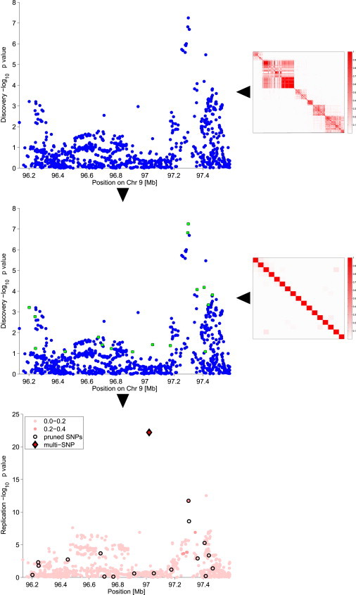
Brief Summary of the Multi-SNP Locus-Association Method

First, SNPs at the locus were prioritized (on the basis of their discovery p values) and were LD pruned (on the basis of their pairwise LD). The emerging SNPs were taken to validation, where the multi-SNP was created as their optimal linear combination and was tested against the chi-square distribution for obtaining the multi-SNP association p value.

In Silico Analysis

To demonstrate the utility of our method in a controlled setting, we simulated phenotype data by mimicking the imperfect-tagging scenario. To this end, we fixed a genomic region and randomly selected an additively coded SNP g and created a phenotype that was additively associated with this SNP. In formula $y=g+\epsilon$, $\epsilon \sim \mathcal{N}\left(0,{\sigma }^2\right)$ with ${\sigma }^2$ = $\text{Var}\left(g\right)·\left(1/r_g^2-1\right)$. This ensures that the explained variance is $r_g^2$.

In this region (±500 kb), we then masked all SNPs whose LD with the causal locus was higher than a certain threshold (ρ). The data (n = 5,000 from the CoLaus study; see Supplemental Data section 9 for further details) were then equally split into discovery and validation parts. We used the discovery data to select those unmasked SNPs whose p value was below a predefined threshold α. We then used the validation data for these SNPs to estimate the EV of the multi-SNP approximating the causal marker according to Equation 1. This estimate was then contrasted with the EV estimate of the top associated observed SNP. This exercise was carried out for various genomic regions, masking thresholds (ρ), strengths of causal association ($r_g^2$), and SNP-selection thresholds (α). For each parameter setup, the phenotype was simulated 1,000 times, and the results were averaged over these repeats.

Application to Meta-analysis Summary Statistics

To apply our multi-SNP association method to the association summary statistics of the GIANT consortium (for height,⁸ BMI,⁹ and WHR¹⁰), we split the studies into two groups of cohorts (total sample size = 81,000 and 47,000) and meta-analyzed each group of studies separately. Note that for further validation purposes, we did not include the CoLaus¹⁵ cohort in this meta-analysis. The first group of studies served as discovery samples, and the second group served as validation samples. Loci were defined as the ±0.5 cM region around each lead SNP. Lead SNPs were selected on the basis of their discovery p values (p < 10⁻²) and were subsequently pruned such that neighboring lead SNPs were forced to be at least 1 cM apart. Note that by definition, the loci do not overlap, which ensured counting each signal only once. Subsequently, at each locus, SNPs below a certain p value threshold (p < 10⁻²) were pruned such that if two SNPs were in LD ($r^2>0.1$), the one with a less significant p value (in the discovery cohort) was thrown away.

For each locus, we estimated the effect size in the validation sample for the selected set of semi-independent SNPs. Finally, we again used the estimate of the correlation matrix (external genotype data) to obtain a lower bound on the EV at each locus.

Results

In Silico Results

First, we simulated a scenario in which a causal variant is imperfectly tagged by masking all SNPs whose LD with the causal marker was higher than a certain threshold. Second, we applied both the standard single-SNP method and our multi-SNP method to estimate the EV of the underlying causal marker.

Figure 2A illustrates how the EV of the multi-SNP increases as a function of increasing discovery p value threshold α (without LD pruning). For completeness, we also explored a wide range of p-value- and pruning-threshold combinations for a fixed simulation scenario (see Supplemental Data section 8) and observed large variations in statistical power. Because the optimal combination is, in reality, not known, we deliberately chose a nonoptimal strategy of α = 2 × 10⁻² combined with no LD pruning for the rest of the simulation experiment. Second, we noticed that the EV of the true causal marker was remarkably well estimated even when many LD friends ($r^2>0.2$) of the causal SNP were masked (Figure 2B). Third, in such poor tagging scenarios, single (lead)-SNP associations yielded ten times smaller EVs than did multi-SNPs (Figure 2C). Finally, associated multi-SNPs were much more closely linked to the causal variant than were top associated single SNPs. In Figure 2D, we plotted the LD (squared correlation) between the causal variant and the multi-SNP, as well as the LD between the causal variant and the best associated SNP (in the discovery sample). These results demonstrate that our multi-SNP-association method offers a substantial benefit over single-SNP associations in the case of imperfect tagging.

Figure 2.

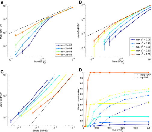
Properties of the Variance Explained by Multi-SNPs

(A) The multi-SNP was generated for various EV values and SNP-selection thresholds (α), whereas all SNPs with an LD $r^2\ge 0.5$ with the casual variant were set unobserved.

(B) The multi-SNP was computed for various EV values ($r_g^2$) and for maximal LD (${\rho }^2$) between the observed SNPs and the causal variant. Here and for the rest of the experiment, we fixed α at 2 × 10⁻².

(C) The EV of the multi-SNP is plotted against that of the best associated observed SNP. The estimates were again generated for various EV values ($r_g^2$) and for maximal LD (${\rho }^2$) between the tagged SNPs and the causal variant. The dotted black line indicates a ten-fold increase.

(D) LD (squared correlation) between the causal SNP and the derived multi-SNP (dashed line) and top associated SNP (solid line). The color coding for (C) and (D) agrees with that of (B).

Application to GIANT Association Summary Statistics

We then tested the multi-SNP method by using the association summary statistics of the GIANT consortium for height,⁸ BMI,⁹ and WHR adjusted for BMI.¹⁰ In order to have both discovery and validation summary statistics for every SNP genome-wide, we partitioned the discovery studies into two groups before meta-analyzing them separately. These two groups represent the discovery and validation samples for the purpose of this paper. We then selected SNPs on the basis of discovery univariate p values and pairwise LD. Then, we combined these SNPs together into a multi-SNP via a multivariate linear regression in the validation sample. Finally, we tested how much phenotypic variance was explained by the multi-SNP and compared this EV to the one explained by single-SNP analysis.

For height, we detected 2,073 loci with a lead-SNP p value < 0.01 in the discovery panel. Because the EV estimates were unbiased and independent (Figures S5 and S6), we could simply sum up the estimates for all 2,073 selected height loci and determine the total fraction of EV. We also calculated the EV by only using the lead SNP from each locus (“single-SNP” analysis). A striking difference was observed between the two estimates (see Table 1): for height, single-SNP associations explained 6.9% of phenotypic variance, whereas the multi-SNPs at the same loci explained 13.5%. Differences for BMI and WHR were slightly less pronounced: single-SNP associations explained 2% and 0.1% of the variance for BMI and WHR, respectively, whereas multi-SNP associations explained 3.6% and 2.2% of the variance for BMI and WHR, respectively, at a locus-selection p value < 0.01. These findings suggest that a non-negligible fraction of the missing heritability—at least for the traits examined in this paper—might be due to multiple independent effects per locus. Note that even if only half of the sample size is used for confirming associations, the multi-SNP method explains more variance than does using the entire sample with just a single-SNP analysis.

Table 1.

TEV of Single SNPs and Multi-SNPs for Each Anthropometric-Trait Phenotype

Trait	p Value	Number of Loci (FDR)	TEV		Number of Replicated Loci
			Single SNP	Multi-SNP	Single SNP	Multi-SNP
Height	p < 5 × 10−8	106 (0.0%)	4.10%	6.93%	93	96
	p < 1 × 10−2	2,073 (80.0%)	6.88%	13.52%	142	186
BMI	p < 5 × 10−8	18 (7.0%)	0.92%	1.02%	15	16
	p < 1 × 10−2	2,031 (95.0%)	1.96%	3.61%	15	25
WHR	p < 5 × 10−8	2 (0.0%)	0.09%	0.09%	2	2
	p < 1 × 10−2	1,985 (100.0%)	0.12%	2.22%	0	2

These estimates account for the number of SNPs constituting the multi-SNP association. FDR was estimated with the Bayes’ theorem (for details, see Supplemental Data section 4). The following abbreviations are used: FDR, false discovery rate; TEV, total explained variance; BMI, body mass index; and WHR, waist-to-hip ratio.

To further demonstrate that our methodology is not biased and also that EV estimates from different loci can be simply summed up, we calculated how much phenotypic variance was explained by all the derived multi-SNPs in the independent CoLaus study,¹⁵ which was not used in either the discovery or the replication samples. Each multi-SNP is a linear combination of its constituting SNPs, and the coefficients are determined on the basis of the replication summary statistics and the SNP correlation matrix (obtained from external cohorts). Knowing these coefficients, we constructed all the multi-SNPs in the CoLaus sample. We then regressed height simultaneously on the 2,073 height-related multi-SNPs and calculated the EV adjusted for the number of variables.¹⁶ We repeated the same exercise for BMI and WHR. The estimates for height and BMI agreed well with those obtained by our method, although the 95% confidence intervals (CIs) were wide because of the relatively small size of the CoLaus sample: 13.2% (CI 10.1%–16.3%) versus 13.5 for height, 2.3% (CI −0.9%–5.6%) versus 3.6 for BMI, and −0.2% (CI −3.4%–3.0%) versus 2.2% for WHR.

For BMI, only loci with small lead-SNP effects harbored allelic heterogeneity, whereas for height, these loci were distributed evenly across the whole spectrum of discovery lead-SNP p values (5 × 10⁻⁸ to 5 × 10⁻²) (Figure 3).

Figure 3.

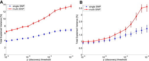
Gain in the TEV for Height and BMI

The TEV of single SNPs and multi-SNPs is plotted as a function of the discovery-p-value cutoff. Although pronounced allelic heterogeneity can be observed throughout the whole p value spectrum for height (A), only SNPs with a smaller effect tend to harbor significant multi-SNPs for BMI (B).

Next, we applied a Benjamini-Hochberg FDR control for the validation p values. For the 2,073 loci, 142 lead SNPs replicated at 5% FDR, whereas 186 multi-SNPs were confirmed at the same FDR. BMI and WHR showed a similar advantage with the use of multi-SNP association (see Table 1).

To establish an inventory of loci with significant evidence of potential allelic heterogeneity, we formally tested whether the multi-SNP explains more phenotypic variance than the best individual SNP in the region. The chi-square test we applied here takes into account the number of SNPs that the multi-SNP was created from. For height, BMI, and WHR, 65, 7, and 2 loci, respectively, were classified as exhibiting significant allelic heterogeneity. A detailed list of such loci can be found in Table S4. Here, we only show one example for height association at the 15q26.1 locus (Figure 4).

Figure 4.

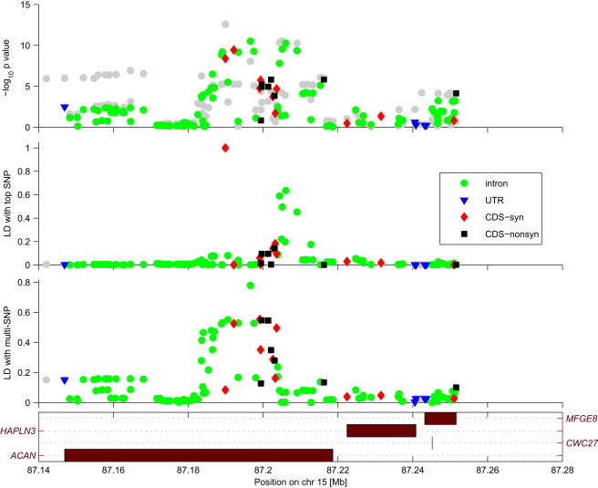
Example of a Height-Associated Locus with Strong Allelic Heterogeneity

The top associated variant is in weak LD with all nonsynonymous markers in ACAN. However, the multi-SNP captures these SNPs.

Given that we were able to estimate the weights assigned to the SNPs that constitute the multi-SNP, we could construct the multi-SNP genotype by using the genotype data of its scaffold SNPs and thus calculate the LD between the multi-SNP and the surrounding SNPs in the region. Figure 4 shows the LD in the region and enables the composite signal of the multi-SNP to be visualized. As can be observed, the association signal is rather broad (top panel); however, not all the signals are due to LD with the lead SNP (middle panel). The multi-SNP encompasses these independent associations and explains most of the observed association in the region (bottom panel). Interestingly, the multi-SNP, unlike the lead SNP, is in strong LD with several missense variants in ACAN (MIM 155760). Not surprisingly, the SNPs picked up by the multi-SNP are predicted to be benign by PolyPhen.¹⁷ Also, a recent Korean exome-sequencing study found a height-associated, nonsynonymous SNP in ACAN.¹⁸ These observations suggest that we are indeed observing the effect of multiple causal variants.

Application to Lipid Association Summary Statistics

In addition to the anthropometric trait associations, we also tested our method on triglyceride, high-density-lipid, low-density-lipid, and total-cholesterol association summary statistics of the largest-to-date lipid meta-analysis study.¹⁹ Given that we had no access to separate discovery and validation summary statistics in the lipid meta-analysis, we had to adapt our method in order to obtain unbiased estimates for the difference in TEV between single and multi-SNP associations. We chose an approach that is conservative (see Material and Methods). Nevertheless, we were still able to detect a 10%–25% relative increase in TEV for these traits when we used multi-SNP association. Additional results are provided in Supplemental Data section 10.

Robustness

Because the meta-analyses report only univariate SNP associations, we derived multivariate effects by using external data to estimate the LD structure of the selected SNPs at each locus. Given that the LD structure can have a great impact on our results, we compared the EV across six different external studies. These cohorts are of individuals from a diverse spectrum of European ancestry and were genotyped on various platforms (Figure S3). For each locus, the different EV estimates, obtained from the six different LD estimates used in our method, were compared to each other. This comparison showed only a 5% median coefficient of variation (CV) in the EV estimates across the six LD patterns, which demonstrates that our methodology is robust to moderate deviations in the LD structure. Sensitivity analyses showed that less stringent LD pruning thresholds ($r^2>0.3$ and $r^2>0.5$) increased the CV (8% and 10%, respectively).

Discussion

We have developed a methodology that is able to estimate the lower bound of the TEV at a locus, and we show that this is significantly larger than the variance explained by the best SNP at the locus. The method exploits imperfect tagging and allelic heterogeneity. The estimate relies on the univariate effect-size estimates and sample sizes for each available SNP and the correlation structure of the SNPs at the given locus. The estimate can also be interpreted as the EV of the association between a multi-SNP and the particular phenotype. The multi-SNP is a specific linear combination of some measured SNPs at the given locus and enables us to better resolve the association signal.

In silico simulations showed that this approach can better detect causal markers in imperfect-tagging scenarios. Furthermore, we have demonstrated that additional pruning facilitates its application to large meta-analytic studies. We also applied this tool to the meta-analysis summary statistics obtained from the GIANT consortium. The analysis yielded many associated loci and significantly increased the TEV.

A recent paper identified substantial allelic heterogeneity at expression QTLs.²⁰ Also, for autoimmune diseases, the major-histocompatibility-complex region has revealed multiple independent effects.^21–23 The GIANT height paper⁸ looked at secondary associations and distinguished 19 loci in which more than one SNP seemed to influence the phenotype. Remarkably, 11 out of these 19 loci were also among our list of 65 height loci. The nonreplicating loci could be due to insufficient power (because of the halved sample size) or to having too many SNPs included in the multi-SNP in cases where the signal was mainly driven by just two or three SNPs.

A region-based meta-analysis was proposed for the study of individuals deriving from different ethnic groups, and the authors of this study highlighted the need to consider more than just individual SNP associations.²⁴ Their method also encompassed association information across multiple SNPs at a given locus, and significance was assessed by a binomial test. Their method has a different focus of application, and hence is not designed to estimate EV, cannot use meta-analysis summary statistics, does not estimate exact signal localization, and is indifferent to the actual SNPs’ contribution to the combined association signal.

While our work was under review, an independent study also proposed a methodology for addressing conditional and joint SNP analysis in the GWAS framework.¹¹ They also used an external reference sample to derive the LD structure in order to approximate multivariate regression when only univariate summary statistics are given. The authors also used the GIANT summary statistics to demonstrate the utility of their method. There are important differences between their method and ours: (1) We used discovery and validation samples to derive unbiased estimates for the EV of the multi-SNP. Their proposed method used the complete sample and applied a very stringent (genome-wide significant) p value threshold for SNP selection to avoid the winner’s curse phenomenon. (2) Whereas we filtered SNPs on the basis of their marginal association p values and pairwise LD, Yang et al. used an elegant stepwise procedure for SNP selection, but without replication, they could not fully exclude any bias in their estimates. (3) Because we used an independent replication sample, we could apply a less stringent p value threshold and could thus examine many more loci without being restrained by a winner’s curse. The use of an independent replication sample enabled us to calculate an unbiased estimate of the TEV of the model proposed in the discovery stage regardless of the number of false-positive SNPs included in the multi-SNP. We chose to select SNPs on the basis of LD-pruned marginal association p values and accepted that some of them might turn out to be false at the validation stage. Therefore, these two methods are complementary: our method is more suited to detect weaker associations with many possible close-to-optimal model configurations and thus allows for more constituting SNPs, but it is less tailored to detect scenarios in which the phenotype is driven by only a few distinct associated SNPs and not by many other variants at the locus. When applying our method to the anthropometric GWASs of the GIANT consortium, we found more significant multi-SNP associations (n = 65 loci for height) than did the method of Yang et al. (n = 36 loci for height); these loci explain more phenotypic variance (5.3% for our method versus 4.1% for the Yang et al. method). Importantly, 24 out of their 36 loci were also found by our method (hypergeometric test, p = 1.1 × 10⁻²⁹).

Note that even in large studies, we do not have sufficient statistical power to distinguish between the best competing multivariate models. The top model emerging from Yang et al.’s analysis for a given locus is not significantly better than many other models containing slightly different SNPs. Predictors (deterministically) selected from a set of correlated variables (like SNP data for a locus) are highly interchangeable. There is little importance of the actual SNPs selected for the optimal model because many different models can fit the data similarly well. This can be easily demonstrated by MCMC sampling of the model space for any locus with allelic heterogeneity. For this reason, we put more emphasis on the EV of the model than on the actual SNPs constituting the multi-SNP.

Our methodology cannot distinguish between true allelic heterogeneity and multiple independent signals tagging an unobserved variant. We asked, nevertheless, whether any discovered multi-SNP (composed of HapMap SNPs) could be tagging a single SNP present only in the 1000 Genomes catalog. This comparison did not identify such a multi-SNP, indicating that imperfect tagging might be less of an issue for common-variant associations (Figure S7). Note, however, that the LD-pruning step in our procedure slightly reduces the chance of detecting an imperfect-tagging scenario in set-ups where only association summary statistics are available. A similar conclusion was reached by Yang et al.¹¹

We found that loci with higher marker density are slightly more prone to harbor allelic heterogeneity (p = 0.002; see Table S2). A possible reason for this is that better coverage enables our methodology to pick up stronger secondary signals. We also found evidence that more conserved loci exhibit more allelic heterogeneity (p = 2.5 × 10⁻⁴; see Table S3). Although high allelic heterogeneity has been linked to low mutation frequency,²⁵ we did not find a significant difference in minor allele frequency (MAF) between loci with strong versus weak evidence of multiple signals (Student’s t test, p = 0.67). We observed, however, that SNPs constituting the confirmed multi-SNPs (p = 4.66 × 10⁻⁴¹) tended to have a lower MAF (0.17) than expected (0.22).

In some cases, the lead SNP alone might not replicate because of fluctuations in the p values, but our multi-SNP approach can be more robust to such variations. Moreover, using multi-SNP associations could potentially improve the detection of pleiotropy in case multi-SNPs associated with different traits at the same locus at least partially overlap. These instances of pleiotropy would be missed by a standard single-SNP association framework.

An important application of our methodology can be to assess the total contribution of variants in specific candidate genes (or pathways) in order to prioritize them. This would be simply done through the restriction of multi-SNP association to particular genes (or pathways) of interest. A gene-centered GWAS approach was proposed for the assessment of deviations from the local quantile-quantile plot.²⁶ However, this method does not attempt to compute cumulative EV and is not applicable to summary statistics.

Our method is implemented in a MATLAB-package multi-SNP, and we added a multivariate association option to our standalone software QUICKTEST.

In summary, our proposed method of investigating allelic heterogeneity revealed that a substantial fraction of the missing heritability can be explained by this phenomenon.

Web Resources

The URLs for data presented herein are as follows:

• Multi-SNP, http://www3.unil.ch/wpmu/sgg/multiSNP

• QUICKTEST, http://www3.unil.ch/wpmu/sgg/quicktest

References

- 1.Hindorff L.A., Sethupathy P., Junkins H.A., Ramos E.M., Mehta J.P., Collins F.S., Manolio T.A. Potential etiologic and functional implications of genome-wide association loci for human diseases and traits. Proc. Natl. Acad. Sci. USA. 2009;106:9362–9367. doi: 10.1073/pnas.0903103106. [DOI] [PMC free article] [PubMed] [Google Scholar]
- 2.Maher B. Personal genomes: The case of the missing heritability. Nature. 2008;456:18–21. doi: 10.1038/456018a. [DOI] [PubMed] [Google Scholar]
- 3.Manolio T.A., Collins F.S., Cox N.J., Goldstein D.B., Hindorff L.A., Hunter D.J., McCarthy M.I., Ramos E.M., Cardon L.R., Chakravarti A. Finding the missing heritability of complex diseases. Nature. 2009;461:747–753. doi: 10.1038/nature08494. [DOI] [PMC free article] [PubMed] [Google Scholar]
- 4.Yang J., Benyamin B., McEvoy B.P., Gordon S., Henders A.K., Nyholt D.R., Madden P.A., Heath A.C., Martin N.G., Montgomery G.W. Common SNPs explain a large proportion of the heritability for human height. Nat. Genet. 2010;42:565–569. doi: 10.1038/ng.608. [DOI] [PMC free article] [PubMed] [Google Scholar]
- 5.Walters R.G., Jacquemont S., Valsesia A., de Smith A.J., Martinet D., Andersson J., Falchi M., Chen F., Andrieux J., Lobbens S. A new highly penetrant form of obesity due to deletions on chromosome 16p11.2. Nature. 2010;463:671–675. doi: 10.1038/nature08727. [DOI] [PMC free article] [PubMed] [Google Scholar]
- 6.Tomlinson I.P., Carvajal-Carmona L.G., Dobbins S.E., Tenesa A., Jones A.M., Howarth K., Palles C., Broderick P., Jaeger E.E., Farrington S., COGENT Consortium. CORGI Collaborators. EPICOLON Consortium Multiple common susceptibility variants near BMP pathway loci GREM1, BMP4, and BMP2 explain part of the missing heritability of colorectal cancer. PLoS Genet. 2011;7:e1002105. doi: 10.1371/journal.pgen.1002105. [DOI] [PMC free article] [PubMed] [Google Scholar]
- 7.Audrézet M.P., Chen J.M., Raguénès O., Chuzhanova N., Giteau K., Le Maréchal C., Quéré I., Cooper D.N., Férec C. Genomic rearrangements in the CFTR gene: Extensive allelic heterogeneity and diverse mutational mechanisms. Hum. Mutat. 2004;23:343–357. doi: 10.1002/humu.20009. [DOI] [PubMed] [Google Scholar]
- 8.Lango Allen H., Estrada K., Lettre G., Berndt S.I., Weedon M.N., Rivadeneira F., Willer C.J., Jackson A.U., Vedantam S., Raychaudhuri S. Hundreds of variants clustered in genomic loci and biological pathways affect human height. Nature. 2010;467:832–838. doi: 10.1038/nature09410. [DOI] [PMC free article] [PubMed] [Google Scholar]
- 9.Speliotes E.K., Willer C.J., Berndt S.I., Monda K.L., Thorleifsson G., Jackson A.U., Lango Allen H., Lindgren C.M., Luan J., Mägi R., MAGIC. Procardis Consortium Association analyses of 249,796 individuals reveal 18 new loci associated with body mass index. Nat. Genet. 2010;42:937–948. doi: 10.1038/ng.686. [DOI] [PMC free article] [PubMed] [Google Scholar]
- 10.Heid I.M., Jackson A.U., Randall J.C., Winkler T.W., Qi L., Steinthorsdottir V., Thorleifsson G., Zillikens M.C., Speliotes E.K., Mägi R., MAGIC Meta-analysis identifies 13 new loci associated with waist-hip ratio and reveals sexual dimorphism in the genetic basis of fat distribution. Nat. Genet. 2010;42:949–960. doi: 10.1038/ng.685. [DOI] [PMC free article] [PubMed] [Google Scholar]
- 11.Yang J., Ferreira T., Morris A.P., Medland S.E., Madden P.A., Heath A.C., Martin N.G., Montgomery G.W., Weedon M.N., Loos R.J., Genetic Investigation of ANthropometric Traits (GIANT) Consortium. DIAbetes Genetics Replication And Meta-analysis (DIAGRAM) Consortium Conditional and joint multiple-SNP analysis of GWAS summary statistics identifies additional variants influencing complex traits. Nat. Genet. 2012;44:369–375. doi: 10.1038/ng.2213. S1–S3. [DOI] [PMC free article] [PubMed] [Google Scholar]
- 12.Benjamini Y., Hochberg Y. Controlling the false discovery rate: A practical and powerful approach to multiple testing. Journal of the Royal Statistical Society Series B (Methodological) 1995;57:289–300. [Google Scholar]
- 13.Cheney W., Kincaid D. Sixth Edition. Thomson; Belmont, U.S.A.: 2007. Numerical Mathematics and Computing. [Google Scholar]
- 14.Harrel F.E., editor. Regression modeling strategies: With Applications to Linear Models, Logistic Regression, and Survival Analysis. First Edition. Springer-Verlag; New York: 2010. [Google Scholar]
- 15.Firmann M., Mayor V., Vidal P.M., Bochud M., Pécoud A., Hayoz D., Paccaud F., Preisig M., Song K.S., Yuan X. The CoLaus study: A population-based study to investigate the epidemiology and genetic determinants of cardiovascular risk factors and metabolic syndrome. BMC Cardiovasc. Disord. 2008;8:6. doi: 10.1186/1471-2261-8-6. [DOI] [PMC free article] [PubMed] [Google Scholar]
- 16.Theil H. North-Holland Publishing Company; Amsterdam: 1961. Economic forecasts and policy. Contributions to economic analysis. [Google Scholar]
- 17.Sunyaev S., Ramensky V., Koch I., Lathe W., 3rd, Kondrashov A.S., Bork P. Prediction of deleterious human alleles. Hum. Mol. Genet. 2001;10:591–597. doi: 10.1093/hmg/10.6.591. [DOI] [PubMed] [Google Scholar]
- 18.Kim J.J., Park Y.M., Baik K.H., Choi H.Y., Yang G.S., Koh I., Hwang J.A., Lee J., Lee Y.S., Rhee H. Exome sequencing and subsequent association studies identify five amino acid-altering variants influencing human height. Hum. Genet. 2012;131:471–478. doi: 10.1007/s00439-011-1096-4. [DOI] [PubMed] [Google Scholar]
- 19.Teslovich T.M., Musunuru K., Smith A.V., Edmondson A.C., Stylianou I.M., Koseki M., Pirruccello J.P., Ripatti S., Chasman D.I., Willer C.J. Biological, clinical and population relevance of 95 loci for blood lipids. Nature. 2010;466:707–713. doi: 10.1038/nature09270. [DOI] [PMC free article] [PubMed] [Google Scholar]
- 20.Wood A.R., Hernandez D.G., Nalls M.A., Yaghootkar H., Gibbs J.R., Harries L.W., Chong S., Moore M., Weedon M.N., Guralnik J.M. Allelic heterogeneity and more detailed analyses of known loci explain additional phenotypic variation and reveal complex patterns of association. Hum. Mol. Genet. 2011;20:4082–4092. doi: 10.1093/hmg/ddr328. [DOI] [PMC free article] [PubMed] [Google Scholar]
- 21.Nejentsev S., Howson J.M., Walker N.M., Szeszko J., Field S.F., Stevens H.E., Reynolds P., Hardy M., King E., Masters J., Wellcome Trust Case Control Consortium Localization of type 1 diabetes susceptibility to the MHC class I genes HLA-B and HLA-A. Nature. 2007;450:887–892. doi: 10.1038/nature06406. [DOI] [PMC free article] [PubMed] [Google Scholar]
- 22.Orozco G., Hinks A., Eyre S., Ke X., Gibbons L.J., Bowes J., Flynn E., Martin P., Wilson A.G., Bax D.E., Wellcome Trust Case Control Consortium. YEAR consortium Combined effects of three independent SNPs greatly increase the risk estimate for RA at 6q23. Hum. Mol. Genet. 2009;18:2693–2699. doi: 10.1093/hmg/ddp193. [DOI] [PMC free article] [PubMed] [Google Scholar]
- 23.Hor H., Kutalik Z., Dauvilliers Y., Valsesia A., Lammers G.J., Donjacour C.E., Iranzo A., Santamaria J., Peraita Adrados R., Vicario J.L. Genome-wide association study identifies new HLA class II haplotypes strongly protective against narcolepsy. Nat. Genet. 2010;42:786–789. doi: 10.1038/ng.647. [DOI] [PubMed] [Google Scholar]
- 24.Wang X., Liu X., Sim X., Xu H., Khor C.C., Ong R.T., Tay W.T., Suo C., Poh W.T., Ng D.P. A statistical method for region-based meta-analysis of genome-wide association studies in genetically diverse populations. Eur. J. Hum. Genet. 2012;20:469–475. doi: 10.1038/ejhg.2011.219. [DOI] [PMC free article] [PubMed] [Google Scholar]
- 25.Pritchard J.K., Cox N.J. The allelic architecture of human disease genes: Common disease-common variant…or not? Hum. Mol. Genet. 2002;11:2417–2423. doi: 10.1093/hmg/11.20.2417. [DOI] [PubMed] [Google Scholar]
- 26.Liu J.Z., McRae A.F., Nyholt D.R., Medland S.E., Wray N.R., Brown K.M., Hayward N.K., Montgomery G.W., Visscher P.M., Martin N.G., Macgregor S., AMFS Investigators A versatile gene-based test for genome-wide association studies. Am. J. Hum. Genet. 2010;87:139–145. doi: 10.1016/j.ajhg.2010.06.009. [DOI] [PMC free article] [PubMed] [Google Scholar]
Associated Data
This section collects any data citations, data availability statements, or supplementary materials included in this article.