

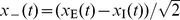
Abstract
Correlations in spike-train ensembles can seriously impair the encoding of information by their spatio-temporal structure. An inevitable source of correlation in finite neural networks is common presynaptic input to pairs of neurons. Recent studies demonstrate that spike correlations in recurrent neural networks are considerably smaller than expected based on the amount of shared presynaptic input. Here, we explain this observation by means of a linear network model and simulations of networks of leaky integrate-and-fire neurons. We show that inhibitory feedback efficiently suppresses pairwise correlations and, hence, population-rate fluctuations, thereby assigning inhibitory neurons the new role of active decorrelation. We quantify this decorrelation by comparing the responses of the intact recurrent network (feedback system) and systems where the statistics of the feedback channel is perturbed (feedforward system). Manipulations of the feedback statistics can lead to a significant increase in the power and coherence of the population response. In particular, neglecting correlations within the ensemble of feedback channels or between the external stimulus and the feedback amplifies population-rate fluctuations by orders of magnitude. The fluctuation suppression in homogeneous inhibitory networks is explained by a negative feedback loop in the one-dimensional dynamics of the compound activity. Similarly, a change of coordinates exposes an effective negative feedback loop in the compound dynamics of stable excitatory-inhibitory networks. The suppression of input correlations in finite networks is explained by the population averaged correlations in the linear network model: In purely inhibitory networks, shared-input correlations are canceled by negative spike-train correlations. In excitatory-inhibitory networks, spike-train correlations are typically positive. Here, the suppression of input correlations is not a result of the mere existence of correlations between excitatory (E) and inhibitory (I) neurons, but a consequence of a particular structure of correlations among the three possible pairings (EE, EI, II).
Author Summary
The spatio-temporal activity pattern generated by a recurrent neuronal network can provide a rich dynamical basis which allows readout neurons to generate a variety of responses by tuning the synaptic weights of their inputs. The repertoire of possible responses and the response reliability become maximal if the spike trains of individual neurons are uncorrelated. Spike-train correlations in cortical networks can indeed be very small, even for neighboring neurons. This seems to be at odds with the finding that neighboring neurons receive a considerable fraction of inputs from identical presynaptic sources constituting an inevitable source of correlation. In this article, we show that inhibitory feedback, abundant in biological neuronal networks, actively suppresses correlations. The mechanism is generic: It does not depend on the details of the network nodes and decorrelates networks composed of excitatory and inhibitory neurons as well as purely inhibitory networks. For the case of the leaky integrate-and-fire model, we derive the correlation structure analytically. The new toolbox of formal linearization and a basis transformation exposing the feedback component is applicable to a range of biological systems. We confirm our analytical results by direct simulations.
Introduction
Neurons generate signals by weighting and combining input spike trains from
presynaptic neuron populations. The number of possible signals which can be read out
this way from a given spike-train ensemble is maximal if these spike trains span an
orthogonal basis, i.e. if they are uncorrelated [1]. If they are correlated, the
amount of information which can be encoded in the spatio-temporal structure of these
spike trains is limited. In addition, correlations impair the ability of readout
neurons to decode information reliably in the presence of noise. This is often
discussed in the context of rate coding: for  uncorrelated spike trains, the signal-to-noise ratio of the
compound spike-count signal can be enhanced by increasing the population size
uncorrelated spike trains, the signal-to-noise ratio of the
compound spike-count signal can be enhanced by increasing the population size
 . In the presence of
correlations, however, the signal-to-noise ratio is bounded [2], [3]. The same reasoning holds for
any other linear combination of spike trains, also for those where exact spike
timing matters (for example for the coding scheme presented in [4]). Thus, the robustness of
neuronal responses against noise critically depends on the level of correlated
activity within the presynaptic neuron population.
. In the presence of
correlations, however, the signal-to-noise ratio is bounded [2], [3]. The same reasoning holds for
any other linear combination of spike trains, also for those where exact spike
timing matters (for example for the coding scheme presented in [4]). Thus, the robustness of
neuronal responses against noise critically depends on the level of correlated
activity within the presynaptic neuron population.
Several studies suggested that correlated neural activity could be beneficial for information processing: Spike-train correlations can modulate the gain of postsynaptic neurons and thereby constitute a gating mechanism (for a review, see [4]). Coherent spiking activity might serve as a means to bind elementary representations into more complex objects [5], [6]. Information represented by correlated firing can be reliably sustained and propagated through feedforward subnetworks (‘synfire chains’; [7], [8]). Whether correlated firing has to be considered favorable or not largely depends on the underlying hypothesis, the type of correlation (e.g. the time scale or the affected frequency band) or which subpopulations of neurons are involved. Most ideas suggesting a functional benefit of correlated activity rely on the existence of an asynchronous ‘ground state’. Spontaneously emerging correlations, i.e. correlations which are not triggered by internal or external events, would impose a serious challenge to many of these hypotheses. Functionally relevant synfire activity, for example, cannot be guaranteed in the presence of correlated background input from the embedding network [9]. It is therefore–from several perspectives–important to understand the origin of uncorrelated activity in neural networks.
It has recently been shown that spike trains of neighboring cortical neurons can indeed be uncorrelated [10]. Similar results have been obtained in several theoretical studies [11]–[17]. From an anatomical point of view, this observation is puzzling: in general, neurons in finite networks share a certain fraction of their presynaptic sources. In particular for neighboring neurons, the overlap between presynaptic neuron populations is expected to be substantial. This feedforward picture suggests that such presynaptic overlap gives rise to correlated synaptic input and, in turn, to correlated response spike trains.
A number of theoretical studies showed that shared-input correlations are only weakly transferred to the output side as a consequence of the nonlinearity of the spike-generation dynamics [15], [18]–[21]. Unreliable spike transmission due to synaptic failure can further suppress the correlation gain [22]. In [9], we demonstrated that spike-train correlations in finite-size recurrent networks are even smaller than predicted by the low correlation gain of pairs of neurons with nonlinear spike-generation dynamics. We concluded that this suppression of correlations must be a result of the recurrent network dynamics. In this article, we compare correlations observed in feedforward networks to correlations measured in systems with an intact feedback loop. We refer to the reduction of correlations in the presence of feedback as “decorrelation”. Different mechanisms underlying such a dynamical decorrelation have been suggested in the recent past. Asynchronous states in recurrent neural networks are often attributed to chaotic dynamics [23], [24]. In fact, networks of nonlinear units with random connectivity and balanced excitation and inhibition typically exhibit chaos [11], [25]. The high sensitivity to noise may however question the functional relevance of such systems ([26], [27]; cf., however, [28]). [29] and [27] demonstrated that asynchronous irregular firing can also emerge in networks with stable dynamics. Employing an analytical framework of correlations in recurrent networks of binary neurons [30], the balance of excitation and inhibition has recently been proposed as another decorrelation mechanism [17]: In large networks, fluctuations of excitation and inhibition are in phase. Positive correlations between excitatory and inhibitory input spike trains lead to a negative component in the net input correlation which can compensate positive correlations caused by shared input.
In the present study, we demonstrate that dynamical decorrelation is a fundamental phenomenon in recurrent systems with negative feedback. We show that negative feedback alone is sufficient to efficiently suppress correlations. Even in purely inhibitory networks, shared-input correlations are compensated by feedback. A balance of excitation and inhibition is thus not required. The underlying mechanism can be understood by means of a simple linear model. This simplifies the theory and helps to gain intuition, but it also confirms that low correlations can emerge in recurrent networks with stable, non-chaotic dynamics.
The suppression of pairwise spike-train correlations by inhibitory feedback is
reflected in a reduction of population-rate fluctuations. The main effect described
in this article can therefore be understood by studying the dynamics of the
macroscopic population activity. This approach leads to a simple mathematical
description and emphasizes that the described decorrelation mechanism is a general
phenomenon which may occur not only in neural networks but also in other
(biological) systems with inhibitory feedback. In “
Results
: Suppression of
population-rate fluctuations in LIF networks”, we first illustrate
the decorrelation effect for random networks of  leaky integrate-and-fire (LIF) neurons with inhibitory or
excitatory-inhibitory coupling. By means of simulations, we show that low-frequency
spike-train correlations, and, hence, population-rate fluctuations are substantially
smaller than expected given the amount of shared input. As shown in the subsequent
section, the “Suppression of population-activity fluctuations by
negative feedback” can readily be understood in the framework of a
simple one-dimensional linear model with negative feedback. In
“
Results
: Population-activity fluctuations in
excitatory-inhibitory networks”, we extend this to a two-population
system with excitatory-inhibitory coupling. Here, a simple coordinate transform
exposes the inherent negative feedback loop as the underlying cause of the
fluctuation suppression in inhibition-dominated networks. The population-rate models
of the inhibitory and the excitatory-inhibitory network are sufficient to understand
the basic mechanism underlying the decorrelation. They do, however, not describe how
feedback in cortical networks affects the detailed structure of pairwise
correlations. In “
Results
: Population averaged correlations in
cortical networks”, we therefore compute self-consistent population
averaged correlations for a random network of
leaky integrate-and-fire (LIF) neurons with inhibitory or
excitatory-inhibitory coupling. By means of simulations, we show that low-frequency
spike-train correlations, and, hence, population-rate fluctuations are substantially
smaller than expected given the amount of shared input. As shown in the subsequent
section, the “Suppression of population-activity fluctuations by
negative feedback” can readily be understood in the framework of a
simple one-dimensional linear model with negative feedback. In
“
Results
: Population-activity fluctuations in
excitatory-inhibitory networks”, we extend this to a two-population
system with excitatory-inhibitory coupling. Here, a simple coordinate transform
exposes the inherent negative feedback loop as the underlying cause of the
fluctuation suppression in inhibition-dominated networks. The population-rate models
of the inhibitory and the excitatory-inhibitory network are sufficient to understand
the basic mechanism underlying the decorrelation. They do, however, not describe how
feedback in cortical networks affects the detailed structure of pairwise
correlations. In “
Results
: Population averaged correlations in
cortical networks”, we therefore compute self-consistent population
averaged correlations for a random network of  linear excitatory and inhibitory neurons. By determining the parameters of the
linear network analytically from the LIF model, we show that the predictions of the
linear model are—for a wide and realistic range of parameters—in
excellent agreement with the results of the LIF network model. In
“
Results
: Effect of feedback
manipulations”, we demonstrate that the active decorrelation in
random LIF networks relies on the feedback of the (sub)population averaged activity
but not on the precise microscopic structure of the feedback signal. In the
“
Discussion
”, we put the consequences of
this work into a broader context and point out limitations and possible extensions
of the presented theory. The “
Methods
” contain details on the LIF
network model, the derivation of the linear model from the LIF dynamics and the
derivation of population-rate spectra and population averaged correlations in the
framework of the linear model. This section is meant as a supplement; the basic
ideas and the main results can be extracted from the “
Results
”.
linear excitatory and inhibitory neurons. By determining the parameters of the
linear network analytically from the LIF model, we show that the predictions of the
linear model are—for a wide and realistic range of parameters—in
excellent agreement with the results of the LIF network model. In
“
Results
: Effect of feedback
manipulations”, we demonstrate that the active decorrelation in
random LIF networks relies on the feedback of the (sub)population averaged activity
but not on the precise microscopic structure of the feedback signal. In the
“
Discussion
”, we put the consequences of
this work into a broader context and point out limitations and possible extensions
of the presented theory. The “
Methods
” contain details on the LIF
network model, the derivation of the linear model from the LIF dynamics and the
derivation of population-rate spectra and population averaged correlations in the
framework of the linear model. This section is meant as a supplement; the basic
ideas and the main results can be extracted from the “
Results
”.
Results
In a recurrent neural network of size  , each
neuron
, each
neuron  receives in general
inputs from two different types of sources: External inputs
receives in general
inputs from two different types of sources: External inputs  representing the sum of afferents from other brain areas,
and local inputs resulting from the recurrent connectivity within the network.
Depending on their origin, external inputs
representing the sum of afferents from other brain areas,
and local inputs resulting from the recurrent connectivity within the network.
Depending on their origin, external inputs  and
and
 to different neurons
 and
and  can be correlated or not. Throughout this manuscript, we
ignore correlations between these external sources, thereby ensuring that
correlations within the network activity arise from the local connectivity alone and
are not imposed by external inputs [17]. The local inputs feed the network's spiking
activity
can be correlated or not. Throughout this manuscript, we
ignore correlations between these external sources, thereby ensuring that
correlations within the network activity arise from the local connectivity alone and
are not imposed by external inputs [17]. The local inputs feed the network's spiking
activity  back to the network
(we refer to spike train
back to the network
(we refer to spike train  , the
, the  th component of the column vector
  [the superscript “
 ” denotes the transpose], as a sum over
delta-functions centered at the spike times
” denotes the transpose], as a sum over
delta-functions centered at the spike times  :
:
 ; the abstract quantity
‘spike train’ can be considered as being derived from the observable
quantity ‘spike count’
; the abstract quantity
‘spike train’ can be considered as being derived from the observable
quantity ‘spike count’  , the
number of spikes occurring in the time interval
, the
number of spikes occurring in the time interval  , by taking the limit
  :
:
 ). The structure and
weighting of this feedback can be described by the network's connectivity
matrix
). The structure and
weighting of this feedback can be described by the network's connectivity
matrix  (see Fig. 1 A). In a finite network,
the local connectivity typically gives rise to overlapping presynaptic populations:
in a random (Erdös-Rényi) network with connection probability
(see Fig. 1 A). In a finite network,
the local connectivity typically gives rise to overlapping presynaptic populations:
in a random (Erdös-Rényi) network with connection probability
 , for example, each
pair of postsynaptic neurons shares, on average,
, for example, each
pair of postsynaptic neurons shares, on average,  presynaptic sources. For a network size of, say,
 and a connection
probability
and a connection
probability  , this corresponds to a
fairly large number of
, this corresponds to a
fairly large number of  identical inputs. For
other network structures, the amount of shared input may be smaller or larger. Due
to this presynaptic overlap, each pair of neurons receives, to some extent,
correlated input (even if the external inputs are uncorrelated). One might therefore
expect that the network responses
identical inputs. For
other network structures, the amount of shared input may be smaller or larger. Due
to this presynaptic overlap, each pair of neurons receives, to some extent,
correlated input (even if the external inputs are uncorrelated). One might therefore
expect that the network responses  are
correlated as well. In this article, we show that, in the presence of negative
feedback, the effect of shared input caused by the structure of the network is
compensated by its recurrent dynamics.
are
correlated as well. In this article, we show that, in the presence of negative
feedback, the effect of shared input caused by the structure of the network is
compensated by its recurrent dynamics.
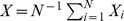
Figure 1. Spiking activity in excitatory-inhibitory LIF networks with intact (left column; feedback scenario) and opened feedback loop (right column; feedforward scenario).

A,B: Network sketches for the feedback (A) and feedforward
scenario (B). C,D: Spiking activity (top panels) and population
averaged firing rate (bottom panels) of the local presynaptic populations.
E,F: Response spiking activity (top panels) and population
averaged response rate (bottom panels). In the top panels of C–F, each
pixel depicts the number of spikes (gray coded) of a subpopulation of
 neurons in a
 time interval.
In both the feedback and the feedforward scenario, the neuron population
time interval.
In both the feedback and the feedforward scenario, the neuron population
 is driven by
the same realization
is driven by
the same realization  of an
uncorrelated white-noise ensemble; local input is fed to the population
through the same connectivity matrix
of an
uncorrelated white-noise ensemble; local input is fed to the population
through the same connectivity matrix  . The in-degrees, the synaptic weights and the
shared-input statistics are thus exactly identical in the two scenarios. In
the feedback case (A), local presynaptic spike-trains are provided by the
network's response
. The in-degrees, the synaptic weights and the
shared-input statistics are thus exactly identical in the two scenarios. In
the feedback case (A), local presynaptic spike-trains are provided by the
network's response  , i.e. the pre- (C) and postsynaptic spike-train
ensembles (E) are identical. In the feedforward scenario (B), the local
presynaptic spike-train population is replaced by an ensemble of
, i.e. the pre- (C) and postsynaptic spike-train
ensembles (E) are identical. In the feedforward scenario (B), the local
presynaptic spike-train population is replaced by an ensemble of
 independent
realizations
independent
realizations  of a Poisson
point process (D). Its rate is identical to the time- and
population-averaged firing rate in the feedback case. See Table 1 and Table 2 for details on
network models and parameters.
of a Poisson
point process (D). Its rate is identical to the time- and
population-averaged firing rate in the feedback case. See Table 1 and Table 2 for details on
network models and parameters.
Suppression of population-rate fluctuations in LIF networks
To illustrate the effect of shared input and its suppression by the recurrent
dynamics, we compare the spike response 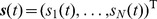 of a recurrent random network (feedback scenario; Fig. 1 A,C,E) of
 LIF neurons to the
case where the feedback is cut and replaced by a spike-train ensemble
LIF neurons to the
case where the feedback is cut and replaced by a spike-train ensemble
 , modeled by
 independent
realizations of a stationary Poisson point process (feedforward
scenario; Fig. 1
B,D,F). The rate of this Poisson process is identical to the time and
population averaged firing rate in the intact recurrent system. In both the
feedback and the feedforward case, the (local) presynaptic spike trains are fed
to the postsynaptic population according to the same connectivity matrix
independent
realizations of a stationary Poisson point process (feedforward
scenario; Fig. 1
B,D,F). The rate of this Poisson process is identical to the time and
population averaged firing rate in the intact recurrent system. In both the
feedback and the feedforward case, the (local) presynaptic spike trains are fed
to the postsynaptic population according to the same connectivity matrix
 . Therefore, not
only the in-degrees and the synaptic weights but also the shared-input
statistics are exactly identical.
. Therefore, not
only the in-degrees and the synaptic weights but also the shared-input
statistics are exactly identical.
For realistic size  and connectivity
 , asynchronous
states of random neural networks [12], [31] exhibit spike-train
correlations which are small but not zero (compare raster displays in Fig. 1 C and D; see also [15]). Although
the presynaptic spike trains are, by construction, independent in the
feedforward case (Fig. 1 D),
the resulting response correlations, and, hence, the population-rate
fluctuations, are substantially stronger than those observed in the feedback
scenario (compare Fig. 1 F and
E). In other words: A theory which is exclusively based on the amount
of shared input but neglects the details of the presynaptic spike-train
statistics can significantly overestimate correlations and population-rate
fluctuations in recurrent neural networks.
, asynchronous
states of random neural networks [12], [31] exhibit spike-train
correlations which are small but not zero (compare raster displays in Fig. 1 C and D; see also [15]). Although
the presynaptic spike trains are, by construction, independent in the
feedforward case (Fig. 1 D),
the resulting response correlations, and, hence, the population-rate
fluctuations, are substantially stronger than those observed in the feedback
scenario (compare Fig. 1 F and
E). In other words: A theory which is exclusively based on the amount
of shared input but neglects the details of the presynaptic spike-train
statistics can significantly overestimate correlations and population-rate
fluctuations in recurrent neural networks.
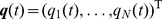
The same effect can be observed in LIF networks with both purely inhibitory and
mixed excitatory-inhibitory coupling (Fig. 2). To demonstrate this quantitatively,
we focus on the fluctuations of the population averaged activity 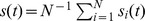 . Its power-spectrum (or auto-correlation, in the time
domain)
. Its power-spectrum (or auto-correlation, in the time
domain)
Figure 2. Suppression of low-frequency fluctuations in recurrent LIF networks
with purely inhibitory (A, C) and mixed excitatory-inhibitory coupling
(B, D) for instantaneous synapses with delay  (A, B) and
low-pass synapses with
(A, B) and
low-pass synapses with  (C, D).

Power-spectra  of
population rates
of
population rates  for the
feedback (black) and the feedforward case (gray; cf. Fig. 1). See Table 1 and Table 2 for details
on network models and parameters. In C and D, local synaptic inputs are
modeled as currents
for the
feedback (black) and the feedforward case (gray; cf. Fig. 1). See Table 1 and Table 2 for details
on network models and parameters. In C and D, local synaptic inputs are
modeled as currents 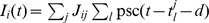 with
with  -function shaped kernel
  with time
constant
with time
constant  (
( denotes
Heaviside function). (Excitatory) Synaptic weights are set to
denotes
Heaviside function). (Excitatory) Synaptic weights are set to
 (see Table 1 for
details). Simulation time
(see Table 1 for
details). Simulation time  . Single-trial spectra smoothed by moving average
(frame size
. Single-trial spectra smoothed by moving average
(frame size  ).
).
 |
(1) |
is determined both by the power-spectra (auto-correlations)  of the individual spike trains and the cross-spectra
(cross-correlations)
of the individual spike trains and the cross-spectra
(cross-correlations)  (
( ) of pairs of spike trains (throughout the article, we
use capital letters to represent quantities in frequency [Fourier]
space;
) of pairs of spike trains (throughout the article, we
use capital letters to represent quantities in frequency [Fourier]
space;  represents the
Fourier transform of the spike train
represents the
Fourier transform of the spike train  ).
We observe that the spike-train power-spectra
).
We observe that the spike-train power-spectra  (and auto-correlations) are barely distinguishable in
the feedback and in the feedforward case (not shown here; the main features of
the spike-train auto-correlation are determined by the average single-neuron
firing rate and the refractory mechanism; both are identical in the feedback and
the feedforward scenario). The differences in the population-rate spectra
(and auto-correlations) are barely distinguishable in
the feedback and in the feedforward case (not shown here; the main features of
the spike-train auto-correlation are determined by the average single-neuron
firing rate and the refractory mechanism; both are identical in the feedback and
the feedforward scenario). The differences in the population-rate spectra
 are therefore
essentially due to differences in the spike-train cross-spectra
are therefore
essentially due to differences in the spike-train cross-spectra  . In other words, the fluctuations in the population
activity serve as a measure of pairwise spike-train correlations [32]: small
(large) population averaged spike-train correlations are accompanied by small
(large) fluctuations in the population rate (see lower panels in Fig. 1 C–F). The
power-spectra
. In other words, the fluctuations in the population
activity serve as a measure of pairwise spike-train correlations [32]: small
(large) population averaged spike-train correlations are accompanied by small
(large) fluctuations in the population rate (see lower panels in Fig. 1 C–F). The
power-spectra  of the population
averaged activity reveal a feedback-induced suppression of the population-rate
variance at low frequencies up to several tens of Hertz. For the examples shown
in Fig. 2, this suppression
spans more than three orders of magnitude for the inhibitory and more than one
order of magnitude for the excitatory-inhibitory network.
of the population
averaged activity reveal a feedback-induced suppression of the population-rate
variance at low frequencies up to several tens of Hertz. For the examples shown
in Fig. 2, this suppression
spans more than three orders of magnitude for the inhibitory and more than one
order of magnitude for the excitatory-inhibitory network.
The suppression of low-frequency fluctuations does not critically depend on the
details of the network model. As shown in Fig. 2, it can, for example, be observed for
both networks with zero rise-time synapses ( -shaped synaptic currents) and short delays and for
networks with delayed low-pass filtering synapses (
-shaped synaptic currents) and short delays and for
networks with delayed low-pass filtering synapses ( -shaped synaptic currents). In the latter case, the
suppression of fluctuations is slightly more restricted to lower frequencies
(
-shaped synaptic currents). In the latter case, the
suppression of fluctuations is slightly more restricted to lower frequencies
( ). Here, the
fluctuation suppression is however similarly pronounced as in networks with
instantaneous synapses.
). Here, the
fluctuation suppression is however similarly pronounced as in networks with
instantaneous synapses.
In Fig. 2 C,D, the
power-spectra of the population activity converge to the mean firing rate at
high frequencies. This indicates that the spike trains are uncorrelated on short
time scales. For instantaneous  -synapses, neurons exhibit an immediate response to
excitatory input spikes [33], [34]. This fast response causes spike-train correlations
on short time scales. Hence, the compound power at high frequencies is
increased. In a recurrent system, this effect is amplified by reverberating
simultaneous excitatory spikes. Therefore, the high-frequency power of the
compound activity is larger in the feedback case (Fig. 2 B). Note that this high-frequency
effect is absent in networks with more realistic low-pass filtering synapses
(Fig. 2 C,D) and in
purely inhibitory networks (Fig. 2
A).
-synapses, neurons exhibit an immediate response to
excitatory input spikes [33], [34]. This fast response causes spike-train correlations
on short time scales. Hence, the compound power at high frequencies is
increased. In a recurrent system, this effect is amplified by reverberating
simultaneous excitatory spikes. Therefore, the high-frequency power of the
compound activity is larger in the feedback case (Fig. 2 B). Note that this high-frequency
effect is absent in networks with more realistic low-pass filtering synapses
(Fig. 2 C,D) and in
purely inhibitory networks (Fig. 2
A).
Synaptic delays and slow synapses can promote oscillatory modes in certain
frequency bands [12], [31], thereby leading to peaks in the population-rate
spectra in the feedback scenario which exceed the power in the feedforward case
(see peaks at  in Fig. 2 C,D). Note that, in the
feedforward case, the local input was replaced by a stationary Poisson process,
whereas in the recurrent network (feedback case) the presynaptic spike trains
exhibit oscillatory modes. By replacing the feedback by an inhomogeneous Poisson
process with a time dependent intensity which is identical to the population
rate in the recurrent network, we found that these oscillatory modes are neither
suppressed nor amplified by the recurrent dynamics, i.e. the peaks in the
resulting power-spectra have the same amplitude in the feedback and in the
feedforward case (data not shown here). At low frequencies, however, the results
are identical to those obtained by replacing the feedback by a homogeneous
Poisson process (i.e. to those shown in Fig. 2; see “
Results
: Effect of
feedback manipulations”). In the present study, we mainly focus
on these low-frequency effects.
in Fig. 2 C,D). Note that, in the
feedforward case, the local input was replaced by a stationary Poisson process,
whereas in the recurrent network (feedback case) the presynaptic spike trains
exhibit oscillatory modes. By replacing the feedback by an inhomogeneous Poisson
process with a time dependent intensity which is identical to the population
rate in the recurrent network, we found that these oscillatory modes are neither
suppressed nor amplified by the recurrent dynamics, i.e. the peaks in the
resulting power-spectra have the same amplitude in the feedback and in the
feedforward case (data not shown here). At low frequencies, however, the results
are identical to those obtained by replacing the feedback by a homogeneous
Poisson process (i.e. to those shown in Fig. 2; see “
Results
: Effect of
feedback manipulations”). In the present study, we mainly focus
on these low-frequency effects.
The observation that the suppression of low-frequency fluctuations is particularly pronounced in networks with purely inhibitory coupling indicates that inhibitory feedback may play a key role for the underlying mechanism. In the following subsection, we demonstrate by means of a one-dimensional linear population model that, indeed, negative feedback alone leads to an efficient fluctuation suppression.
Suppression of population-activity fluctuations by negative feedback
Average pairwise correlations can be extracted from the spectrum (1) of the
compound activity, provided the single spike-train statistics
(auto-correlations) is known (see previous section). As the single spike-train
statistics is identical in the feedback and in the feedforward scenario, the
mechanism underlying the decorrelation in recurrent networks can be understood
by studying the dynamics of the population averaged activity. In this and in the
next subsection, we consider the linearized dynamics of random networks composed
of homogeneous subpopulations of LIF neurons. The high-dimensional dynamics of
such systems can be reduced to low-dimensional models describing the dynamics of
the compound activity (for details, see “
Methods
: Linearized network
model”). Note that this reduction is exact for networks with
homogeneous out-degree (number of outgoing connections). For the networks
studied here (random networks with homogeneous in-degree), it serves as a
sufficient approximation (in a network of size  where each connection is randomly and independently
realized with probability
where each connection is randomly and independently
realized with probability  [Erdös-Rényi graph], the [binomial] in- and
out-degree distributions become very narrow for large
[Erdös-Rényi graph], the [binomial] in- and
out-degree distributions become very narrow for large  [relative to the mean in/out-degree]; both in-
and out-degree are therefore approximately constant across the population of
neurons). In this subsection, we first study networks with purely inhibitory
coupling. In “
Results
: Population-activity fluctuations in
excitatory-inhibitory networks”, we investigate the effect of
mixed excitatory-inhibitory connectivity.
[relative to the mean in/out-degree]; both in-
and out-degree are therefore approximately constant across the population of
neurons). In this subsection, we first study networks with purely inhibitory
coupling. In “
Results
: Population-activity fluctuations in
excitatory-inhibitory networks”, we investigate the effect of
mixed excitatory-inhibitory connectivity.
Consider a random network of  identical neurons with connection probability
  . Each neuron
  receives
  randomly chosen
inputs from the local network with synaptic weights
randomly chosen
inputs from the local network with synaptic weights  . In addition, the neurons are driven by external
uncorrelated Gaussian white noise
. In addition, the neurons are driven by external
uncorrelated Gaussian white noise  with amplitude
  , i.e.
 and
and
 . For small input
fluctuations, the network dynamics can be linearized. This linearization is
based on the averaged response of a single neuron to an incoming spike and
describes the activity of an individual neuron
. For small input
fluctuations, the network dynamics can be linearized. This linearization is
based on the averaged response of a single neuron to an incoming spike and
describes the activity of an individual neuron  by an abstract fluctuating quantity
  which is defined such that within the linear
approximation its auto- and cross-correlations fulfill the same linearized
equation as the spiking model in the low-frequency limit. Consequently, also the
low-frequency fluctuations of the population spike rate are captured correctly
by the reduced model up to linear order. This approach is equivalent to the
treatment of finite-size fluctuations in spiking networks (see, e.g., [31]). For
details, see “
Methods
: Linearized network
model”. For large
which is defined such that within the linear
approximation its auto- and cross-correlations fulfill the same linearized
equation as the spiking model in the low-frequency limit. Consequently, also the
low-frequency fluctuations of the population spike rate are captured correctly
by the reduced model up to linear order. This approach is equivalent to the
treatment of finite-size fluctuations in spiking networks (see, e.g., [31]). For
details, see “
Methods
: Linearized network
model”. For large  ,
the population averaged activity
,
the population averaged activity  can hence be described by a one-dimensional linear system
| (2) |
with linear kernel  , effective
coupling strength
, effective
coupling strength  and the population
averaged noise
and the population
averaged noise  (see
“
Methods
: Linearized network model”
and Fig. 3 B). The coupling
strength
(see
“
Methods
: Linearized network model”
and Fig. 3 B). The coupling
strength  represents the
integrated linear response of the neuron population to a small perturbation in
the input rate of a single presynaptic neuron. For a population of LIF neurons,
its relation to the synaptic weight
represents the
integrated linear response of the neuron population to a small perturbation in
the input rate of a single presynaptic neuron. For a population of LIF neurons,
its relation to the synaptic weight  (PSP amplitude) is derived in “
Methods
: Linearized network
model” and “
Methods
: Response kernel of the LIF
model”. The normalized kernel
(PSP amplitude) is derived in “
Methods
: Linearized network
model” and “
Methods
: Response kernel of the LIF
model”. The normalized kernel  (with
(with  )
captures the time course of the linear response. It is determined by the
single-neuron properties (e.g. the spike-initiation dynamics [35],
[36]),
the properties of the synapses (e.g. synaptic weights and time constants [37], [38]) and the
properties of the input (e.g. excitatory vs. inhibitory input [39]). For
many real and model neurons, the linear population-rate response exhibits
low-pass characteristics [13], [34]–[46]. For illustration (Fig. 3), we consider a
1st-order low-pass filter, i.e. an exponential impulse response
)
captures the time course of the linear response. It is determined by the
single-neuron properties (e.g. the spike-initiation dynamics [35],
[36]),
the properties of the synapses (e.g. synaptic weights and time constants [37], [38]) and the
properties of the input (e.g. excitatory vs. inhibitory input [39]). For
many real and model neurons, the linear population-rate response exhibits
low-pass characteristics [13], [34]–[46]. For illustration (Fig. 3), we consider a
1st-order low-pass filter, i.e. an exponential impulse response  with time constant
  (cutoff frequency
  ;
see Fig. 3 A, light gray
curve in E). The results of our analysis are however independent of the choice
of the kernel
;
see Fig. 3 A, light gray
curve in E). The results of our analysis are however independent of the choice
of the kernel  . The
auto-correlation
. The
auto-correlation  of the external
noise is parametrized by the effective noise amplitude
of the external
noise is parametrized by the effective noise amplitude  .
.
Figure 3. Partial canceling of fluctuations in a linear system by inhibitory feedback.

Response  of a
linear system with impulse response
of a
linear system with impulse response  (1st-order
low-pass, cutoff frequency
(1st-order
low-pass, cutoff frequency  ) to Gaussian white noise input
  with
amplitude
with
amplitude  for three
local-input scenarios. A (light gray): No feedback (local
input
for three
local-input scenarios. A (light gray): No feedback (local
input  ).
B (black): Negative feedback (
).
B (black): Negative feedback ( ) with
strength
) with
strength  . The
fluctuations of the weighted local input
. The
fluctuations of the weighted local input  (B
(B ) are
anticorrelated to the external drive
) are
anticorrelated to the external drive  (B
(B ).
C (dark gray): Feedback in B is replaced by
uncorrelated feedforward input
).
C (dark gray): Feedback in B is replaced by
uncorrelated feedforward input  with the same auto-statistics as the response
 in
B
in
B . The local
input
. The local
input  is
constructed by assigning a random phase
is
constructed by assigning a random phase  to each
Fourier component
to each
Fourier component  of the
response in B
of the
response in B .
Fluctuations in C
.
Fluctuations in C and
C
and
C are
uncorrelated. A, B, C: Network
sketches. A
are
uncorrelated. A, B, C: Network
sketches. A
 , B
, B
 ,
C
,
C
 : External
input
: External
input  .
A
.
A
 ,
B
,
B
 ,
C
,
C
 : Weighted
local input
: Weighted
local input  .
A
.
A
 ,
B
,
B
 ,
C
,
C
 : Responses
 .
D, E: Response auto-correlation functions
(D) and power-spectra (E) for the three cases shown in A,B,C (same gray
coding as in A,B,C; inset in D: normalized auto-correlations).
.
D, E: Response auto-correlation functions
(D) and power-spectra (E) for the three cases shown in A,B,C (same gray
coding as in A,B,C; inset in D: normalized auto-correlations).
Given the simplified description (2), the suppression of response fluctuations by
negative feedback can be understood intuitively: Consider first the case where
the neurons in the local network are unconnected (Fig. 3 A; no feedback,  ). Here, the response
  (Fig. 3
A
(Fig. 3
A
 ) is simply a
low-pass filtered version of the external input
) is simply a
low-pass filtered version of the external input  (Fig. 3
A
(Fig. 3
A
 ), resulting in an
exponentially decaying response auto-correlation (Fig. 3 D; light gray curve) and a drop in the
response power-spectrum at the cutoff frequency
), resulting in an
exponentially decaying response auto-correlation (Fig. 3 D; light gray curve) and a drop in the
response power-spectrum at the cutoff frequency  (Fig. 3
E). At low frequencies,
(Fig. 3
E). At low frequencies,  and
and  are in phase; they
are correlated. In the presence of negative feedback (Fig. 3 B), the local input
are in phase; they
are correlated. In the presence of negative feedback (Fig. 3 B), the local input  (Fig. 3
B
(Fig. 3
B
 ) and the
low-frequency components of the external input
) and the
low-frequency components of the external input  (Fig. 3
B
(Fig. 3
B
 ) are
anticorrelated. They partly cancel out, thereby reducing the response
fluctuations
) are
anticorrelated. They partly cancel out, thereby reducing the response
fluctuations  (Fig. 3 B
 ). The auto-correlation function and the power-spectrum
are suppressed (Fig. 3 D,E;
black curves). Due to the low-pass characteristics of the system, mainly the
low-frequency components of the external drive
). The auto-correlation function and the power-spectrum
are suppressed (Fig. 3 D,E;
black curves). Due to the low-pass characteristics of the system, mainly the
low-frequency components of the external drive  are transferred to the output side and, in turn, become
available for the feedback signal. Therefore, the canceling of input
fluctuations and the resulting suppression of response fluctuations are most
efficient at low frequencies. Consequently, the auto-correlation function is
sharpened (see inset in Fig. 3
D). The cutoff frequency of the system is increased (Fig. 3 E; black curve). This
effect of negative feedback is very general and well known in the engineering
literature. It is employed in the design of technical devices, like, e.g.,
amplifiers [47]. As the zero-frequency power is identical to the
integrated auto-correlation function, the suppression of low-frequency
fluctuations is accompanied by a reduction in the auto-correlation area (Fig. 3 D; black curve). Note
that the suppression of fluctuations in the feedback case is not merely a result
of the additional inhibitory noise source provided by the local input, but
follows from the precise temporal alignment of the local and the external input.
To illustrate this, let's consider the case where the feedback channel is
replaced by a feedforward input
are transferred to the output side and, in turn, become
available for the feedback signal. Therefore, the canceling of input
fluctuations and the resulting suppression of response fluctuations are most
efficient at low frequencies. Consequently, the auto-correlation function is
sharpened (see inset in Fig. 3
D). The cutoff frequency of the system is increased (Fig. 3 E; black curve). This
effect of negative feedback is very general and well known in the engineering
literature. It is employed in the design of technical devices, like, e.g.,
amplifiers [47]. As the zero-frequency power is identical to the
integrated auto-correlation function, the suppression of low-frequency
fluctuations is accompanied by a reduction in the auto-correlation area (Fig. 3 D; black curve). Note
that the suppression of fluctuations in the feedback case is not merely a result
of the additional inhibitory noise source provided by the local input, but
follows from the precise temporal alignment of the local and the external input.
To illustrate this, let's consider the case where the feedback channel is
replaced by a feedforward input  (Fig. 3 C) which has the
same auto-statistics as the response
(Fig. 3 C) which has the
same auto-statistics as the response  in the feedback case (Fig. 3
B
in the feedback case (Fig. 3
B
 ) but is
uncorrelated to the external drive
) but is
uncorrelated to the external drive  .
In this case, external input fluctuations (Fig. 3 C
.
In this case, external input fluctuations (Fig. 3 C
 ) are not canceled by the local input
  (Fig. 3
C
(Fig. 3
C
 ). Instead, the
local feedforward input acts as an additional noise source which leads to an
increase in the response fluctuations (Fig. 3 C
). Instead, the
local feedforward input acts as an additional noise source which leads to an
increase in the response fluctuations (Fig. 3 C
 ). The response auto-correlation and power-spectrum
(Fig. 3 D,E; dark gray
curves) are increased. Compared to the unconnected case (Fig. 3 E; light gray curve), the cutoff
frequency remains unchanged.
). The response auto-correlation and power-spectrum
(Fig. 3 D,E; dark gray
curves) are increased. Compared to the unconnected case (Fig. 3 E; light gray curve), the cutoff
frequency remains unchanged.
The feedback induced suppression of response fluctuations can be quantified by comparing the response power-spectra
| (3) |
and
| (4) |
in the feedback (Fig. 3 B)
and the feedforward case (Fig. 3
C), respectively (see “
Methods
: Population-activity spectrum of
the linear inhibitory network”). Here,  and
and  denote the Fourier transforms of the response fluctuations in the feedback and
the feedforward scenario, respectively,
denote the Fourier transforms of the response fluctuations in the feedback and
the feedforward scenario, respectively,  the transfer function (Fourier transform of the filter kernel
  ) of the neuron population, and
  the average across noise realizations. We use the power
ratio
the average across noise realizations. We use the power
ratio
| (5) |
as a measure of the relative fluctuation suppression caused by feedback. For low
frequencies ( ) and strong
effective coupling
) and strong
effective coupling  , the power ratio
(5) decays as
, the power ratio
(5) decays as  (see Fig. 4 A): the suppression of
population-rate fluctuations is promoted by strong negative feedback. In line
with the observations in “
Results
: Suppression of population-rate
fluctuations in LIF networks”, this suppression is restricted
to low frequencies; for high frequencies (
(see Fig. 4 A): the suppression of
population-rate fluctuations is promoted by strong negative feedback. In line
with the observations in “
Results
: Suppression of population-rate
fluctuations in LIF networks”, this suppression is restricted
to low frequencies; for high frequencies ( ,
i.e.
,
i.e.  ), the power ratio
 approaches
 . Note that the
power ratio (5) is independent of the amplitude
. Note that the
power ratio (5) is independent of the amplitude  of the population averaged external input
 . Therefore, even
if we dropped the assumption of the external inputs
. Therefore, even
if we dropped the assumption of the external inputs  being uncorrelated, i.e. if
  for
for  ,
the power ratio (5) remained the same. For correlated external input, the power
,
the power ratio (5) remained the same. For correlated external input, the power
 of the population
average
of the population
average  is different from
 . The suppression
factor
. The suppression
factor  , however, is not
affected by this. Moreover, it is straightforward to show that the power ratio
(5) is, in fact, independent of the shape of the external-noise spectrum
, however, is not
affected by this. Moreover, it is straightforward to show that the power ratio
(5) is, in fact, independent of the shape of the external-noise spectrum
 . The same result
(5) is obtained for any type of external input (e.g. colored noise or
oscillating inputs).
. The same result
(5) is obtained for any type of external input (e.g. colored noise or
oscillating inputs).
Figure 4. Suppression of low-frequency (LF) population-rate fluctuations in linearized homogeneous random networks with purely inhibitory (A) and mixed excitatory-inhibitory coupling (B).

Dependence of the zero-frequency power ratio  on the
effective coupling strength
on the
effective coupling strength  (solid curves: full solutions; dashed lines:
strong-coupling approximations). The power ratio
(solid curves: full solutions; dashed lines:
strong-coupling approximations). The power ratio  represents
the ratio between the low-frequency population-rate power in the
recurrent networks (A: Fig. 3 B; B: Fig. 5 A,B) and in
networks where the feedback channels are replaced by uncorrelated
feedforward input (A: Fig. 3 C; B, black:
Fig. 5 C,D;
B, gray: Fig. 5 D′). Dotted curves in B depict
power ratio of the sum modes
represents
the ratio between the low-frequency population-rate power in the
recurrent networks (A: Fig. 3 B; B: Fig. 5 A,B) and in
networks where the feedback channels are replaced by uncorrelated
feedforward input (A: Fig. 3 C; B, black:
Fig. 5 C,D;
B, gray: Fig. 5 D′). Dotted curves in B depict
power ratio of the sum modes  and
and  (see text). B: Balance factor
  .
.
For low frequencies, the transfer function  approaches unity (
 ); the exact shape
of the kernel
); the exact shape
of the kernel  becomes
irrelevant. In particular, the cutoff frequency (or time constant) of a low-pass
kernel has no effect on the zero-frequency power (integral correlation) and the
zero-frequency power ratio
becomes
irrelevant. In particular, the cutoff frequency (or time constant) of a low-pass
kernel has no effect on the zero-frequency power (integral correlation) and the
zero-frequency power ratio  (Fig. 4). Therefore, the
suppression of low-frequency fluctuations does not critically depend on the
exact choice of the neuron, synapse or input model. The same reasoning applies
to synaptic delays: Replacing the kernel
(Fig. 4). Therefore, the
suppression of low-frequency fluctuations does not critically depend on the
exact choice of the neuron, synapse or input model. The same reasoning applies
to synaptic delays: Replacing the kernel  by a delayed kernel
  leads to an
additional phase factor
leads to an
additional phase factor  in the transfer
function
in the transfer
function  . For sufficiently
small frequencies (long time scales), this factor can be neglected
(
. For sufficiently
small frequencies (long time scales), this factor can be neglected
( ).
).
For networks with purely inhibitory feedback, the absolute power (3) of the
population rate decreases monotonously with increasing coupling strength
 . As we will
demonstrate in “
Results
: Population-activity fluctuations in
excitatory-inhibitory networks” and “
Results
: Population
averaged correlations in cortical networks”, this is
qualitatively different in networks with mixed excitatory and inhibitory
coupling
. As we will
demonstrate in “
Results
: Population-activity fluctuations in
excitatory-inhibitory networks” and “
Results
: Population
averaged correlations in cortical networks”, this is
qualitatively different in networks with mixed excitatory and inhibitory
coupling  and
and
 , respectively:
here, the fluctuations of the compound activity increase with
, respectively:
here, the fluctuations of the compound activity increase with  . The power ratio
  ,
however, still decreases with
,
however, still decreases with  .
.
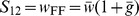
Population-activity fluctuations in excitatory-inhibitory networks
In the foregoing subsection, we have shown that negative feedback alone can
efficiently suppress population-rate fluctuations and, hence, spike-train
correlations. So far, it is unclear whether the same reasoning applies to
networks with mixed excitatory and inhibitory coupling. To clarify this, we now
consider a random network composed of a homogeneous excitatory and inhibitory
subpopulation  and
and
 of size
 and
and
 , respectively.
Each neuron receives
, respectively.
Each neuron receives  excitatory and
 inhibitory inputs
from
inhibitory inputs
from  and
and
 with synaptic
weights
with synaptic
weights  and
and
 , respectively. In
addition, the neurons are driven by external Gaussian white noise. As
demonstrated in “
Methods
: Linearized network
model”, linearization and averaging across subpopulations leads
to a two-dimensional system
, respectively. In
addition, the neurons are driven by external Gaussian white noise. As
demonstrated in “
Methods
: Linearized network
model”, linearization and averaging across subpopulations leads
to a two-dimensional system
| (6) |
describing the linearized dynamics of the subpopulation averaged activity
 . Here,
 denotes the
subpopulation averaged external uncorrelated white-noise input with correlation
functions
denotes the
subpopulation averaged external uncorrelated white-noise input with correlation
functions  (
( ,
,  ), and
 a normalized
linear kernel with
a normalized
linear kernel with  . The excitatory
and inhibitory subpopulations are coupled through an effective connectivity
matrix
. The excitatory
and inhibitory subpopulations are coupled through an effective connectivity
matrix
| (7) |
with effective weight  and balance
parameter
and balance
parameter  .
.
The two-dimensional system (6)/(7) represents a recurrent system with both positive and negative feedback connections (Fig. 5 A). By introducing new coordinates
Figure 5. Sketch of the 2D (excitatory-inhibitory) model for the feedback (A,B) and the feedforward scenario (C,D) in normal (A,C) and Schur-basis representation (B,D).

A: Original 2D recurrent system. B: Schur-basis
representation of the system shown in A. C: Feedforward
scenario: Excitatory and inhibitory feedback connections of the original
network (A) are replaced by feedforward input from populations with
rates  ,
,
 ,
respectively. D: Schur-basis representation of the system
shown in C. D′: Alternative feedforward scenario:
Here, the feedforward channel (weight
,
respectively. D: Schur-basis representation of the system
shown in C. D′: Alternative feedforward scenario:
Here, the feedforward channel (weight  ) of the
original system in Schur basis (B) remains intact. Only the inhibitory
feedback (weight
) of the
original system in Schur basis (B) remains intact. Only the inhibitory
feedback (weight  ) is
replaced by feedforward input
) is
replaced by feedforward input  .
.
| (8) |
and  ,
,  , we obtain an equivalent representation of (6)/(7),
| (9) |
describing the dynamics of the sum and difference activity  and
and  ,
respectively, i.e. the in- and anti-phase components of the excitatory and
inhibitory subpopulations (see [48]–[50]). The new coupling
matrix
,
respectively, i.e. the in- and anti-phase components of the excitatory and
inhibitory subpopulations (see [48]–[50]). The new coupling
matrix
| (10) |
reveals that the sum mode  is subject to
self-feedback (
is subject to
self-feedback (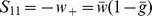 ) and receives
feedforward input from the difference mode
) and receives
feedforward input from the difference mode  (
( ). All remaining
connections are absent (
). All remaining
connections are absent ( ) in the new
representation (8) (see Fig. 5
B). The correlation functions of the external noise in the new
coordinates are given by
) in the new
representation (8) (see Fig. 5
B). The correlation functions of the external noise in the new
coordinates are given by 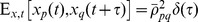 with
with
 (
( ).
).
The feedforward coupling is positive ( ):
an excitation surplus (
):
an excitation surplus ( ) will excite all
neurons in the network, an excitation deficit (
) will excite all
neurons in the network, an excitation deficit ( ) will lead to global inhibition. In inhibition dominated
regimes with
) will lead to global inhibition. In inhibition dominated
regimes with  , the self-feedback
of the sum activity
, the self-feedback
of the sum activity  is effectively
negative (
is effectively
negative ( ). The dynamics of
the sum rate in inhibition-dominated excitatory-inhibitory networks is therefore
qualitatively similar to the dynamics in purely inhibitory networks
(“
Results
: Suppression of population-activity
fluctuations by negative feedback”). As shown below, the
negative feedback loop exposed by the transform (8) leads to an efficient
relative suppression of population-rate fluctuations (if compared to the
feedforward case).
). The dynamics of
the sum rate in inhibition-dominated excitatory-inhibitory networks is therefore
qualitatively similar to the dynamics in purely inhibitory networks
(“
Results
: Suppression of population-activity
fluctuations by negative feedback”). As shown below, the
negative feedback loop exposed by the transform (8) leads to an efficient
relative suppression of population-rate fluctuations (if compared to the
feedforward case).
Mathematically, the coordinate transform (8) corresponds to a Schur
decomposition of the dynamics: Any recurrent system of type (6)
(with arbitrary coupling matrix  )
can be transformed to a system with a triangular coupling matrix (see, e.g.,
[50]). The
resulting coupling between the different Schur modes can be ordered so that
there are only connections from modes with lower index to modes with the same or
larger index. In this sense, the resulting system has been termed
‘feedforward’ [50]. The original coupling matrix
)
can be transformed to a system with a triangular coupling matrix (see, e.g.,
[50]). The
resulting coupling between the different Schur modes can be ordered so that
there are only connections from modes with lower index to modes with the same or
larger index. In this sense, the resulting system has been termed
‘feedforward’ [50]. The original coupling matrix  is typically not normal, i.e.
  . Its eigenvectors do not form an orthogonal basis. By
performing a Gram-Schmidt orthonormalization of the eigenvectors, however, one
can obtain a (normalized) orthogonal basis, a Schur basis. Our new coordinates
(8) correspond to the amplitudes (the time evolution) of two orthogonal Schur
modes.
. Its eigenvectors do not form an orthogonal basis. By
performing a Gram-Schmidt orthonormalization of the eigenvectors, however, one
can obtain a (normalized) orthogonal basis, a Schur basis. Our new coordinates
(8) correspond to the amplitudes (the time evolution) of two orthogonal Schur
modes.
The spectra  ,
,  ,
,  and
and
 of the
subpopulation averaged rates
of the
subpopulation averaged rates  ,
,
 and the sum mode
 , respectively, are
derived in “
Methods
: Population-activity spectra of the
linear excitatory-inhibitory network”. In contrast to the
purely inhibitory network (see “
Results
: Suppression of population-activity
fluctuations by negative feedback”), the population-rate
fluctuations of the excitatory-inhibitory network increase monotonously with
increasing coupling strength
, respectively, are
derived in “
Methods
: Population-activity spectra of the
linear excitatory-inhibitory network”. In contrast to the
purely inhibitory network (see “
Results
: Suppression of population-activity
fluctuations by negative feedback”), the population-rate
fluctuations of the excitatory-inhibitory network increase monotonously with
increasing coupling strength  .
For strong coupling,
.
For strong coupling,  approaches
| (11) |
from below with  . Close to the
critical point (
. Close to the
critical point ( ), the rate
fluctuations become very large; (11) diverges. Increasing the amount of
inhibition by increasing
), the rate
fluctuations become very large; (11) diverges. Increasing the amount of
inhibition by increasing  , however, leads to
a suppression of these fluctuations. In the limit
, however, leads to
a suppression of these fluctuations. In the limit  ,
,  and (11) approach
the spectrum
and (11) approach
the spectrum  of the unconnected
network. For strong coupling (
of the unconnected
network. For strong coupling ( ),
the ratio
),
the ratio  approaches
 : the fluctuations
of the population averaged excitatory firing rate exceed those of the inhibitory
population by a factor
: the fluctuations
of the population averaged excitatory firing rate exceed those of the inhibitory
population by a factor  (independently of
 and
and
 ).
).
Similarly to the strategy we followed in the previous subsections, we will now
compare the population-rate fluctuations of the feedback system (6), or
equivalently (9), to the case where the feedback channels are replaced by
feedforward input with identical auto-statistics. A straight-forward
implementation of this is illustrated in Fig. 5 C: Here, the excitatory and inhibitory
feedback channels  and
and
 are replaced by
uncorrelated feedforward inputs
are replaced by
uncorrelated feedforward inputs  and
and  , respectively. The
Schur representation of this scenario is depicted in Fig. 5 D. According to (6), the Fourier
transforms of the response fluctuations of this system read
, respectively. The
Schur representation of this scenario is depicted in Fig. 5 D. According to (6), the Fourier
transforms of the response fluctuations of this system read
 |
(12) |
With  , and using
 ,
,  ,
,  , we can express
the spectrum
, we can express
the spectrum  of the sum
activity in the feedforward case in terms of the spectra
of the sum
activity in the feedforward case in terms of the spectra  and
and  of the feedback system (see eq. (55)). For strong coupling (
 ), the zero-frequency component (
 ) becomes
| (13) |
Thus, for strong coupling, the zero-frequency power ratio
| (14) |
reveals a relative suppression of the population-rate fluctuations in the
feedback system which is proportional to  (see Fig. 4 B; black dashed
line). The power ratio
(see Fig. 4 B; black dashed
line). The power ratio  for arbitrary
weights
for arbitrary
weights  is depicted in
Fig. 4 B (black dotted
curve). For a network at the transition point
is depicted in
Fig. 4 B (black dotted
curve). For a network at the transition point  , (14) equals
  .
Increasing the level of inhibition by increasing
.
Increasing the level of inhibition by increasing  leads to a decrease in the power ratio: in the limit
 , (14) approaches
 monotonously.
Above, we suggested that the negative self-feedback of the sum mode
 , weighted by
 (Fig. 5 B), is responsible for
the fluctuation suppression in the recurrent excitatory-inhibitory system. Here,
we test this by considering the case where this feedback loop is opened and
replaced by uncorrelated feedforward input
(Fig. 5 B), is responsible for
the fluctuation suppression in the recurrent excitatory-inhibitory system. Here,
we test this by considering the case where this feedback loop is opened and
replaced by uncorrelated feedforward input  , weighted by
  ,
while the feedforward input from the difference mode
,
while the feedforward input from the difference mode  , weighted by
  ,
is left intact (see Fig. 5
D′). As before, we assume that the auto-statistics of
,
is left intact (see Fig. 5
D′). As before, we assume that the auto-statistics of
 is identical to
the auto-statistics of
is identical to
the auto-statistics of  as obtained in the
feedback case, i.e.
as obtained in the
feedback case, i.e. 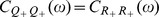 . According to the
Schur representation of the population dynamics (9)/(10), the Fourier transform
of the sum mode of this modified system is given by
. According to the
Schur representation of the population dynamics (9)/(10), the Fourier transform
of the sum mode of this modified system is given by
| (15) |
With  given in (54) and
 , we obtain the
power ratio
, we obtain the
power ratio
| (16) |
Its zero-frequency component  is shown in Fig. 4 B (gray
dotted curve). For strong coupling, the power ratio decays as
is shown in Fig. 4 B (gray
dotted curve). For strong coupling, the power ratio decays as  (gray dashed line in Fig. 4 B). Thus, the (relative) power in the
recurrent system is reduced by strengthening the negative self-feedback loop,
i.e. by increasing
(gray dashed line in Fig. 4 B). Thus, the (relative) power in the
recurrent system is reduced by strengthening the negative self-feedback loop,
i.e. by increasing  .
.
So far, we have presented results for the subpopulation averaged firing rates
 and
and
 and the sum mode
 . The spectrum of
the compound rate
. The spectrum of
the compound rate  , i.e. the activity
averaged across the entire population, reads
, i.e. the activity
averaged across the entire population, reads
 |
(17) |
In the feedforward scenario depicted in Fig. 5 C, the spectrum of the compound rate
 (with
(with
 ) is given by
| (18) |
For strong coupling, the corresponding low-frequency power ratio 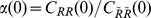 (black solid curve in Fig. 4 B) exhibits qualitatively the same
decrease
(black solid curve in Fig. 4 B) exhibits qualitatively the same
decrease  as the sum
mode.
as the sum
mode.
To summarize the results of this subsection: the population dynamics of a
recurrent network with mixed excitatory and inhibitory coupling can be mapped to
a two-dimensional system describing the dynamics of the sum and the difference
of the excitatory and inhibitory subpopulation activities. This equivalent
representation uncovers that, in inhibition dominated networks ( ), the sum activity is subject to negative self-feedback.
Thus, the dynamics of the sum activity in excitatory-inhibitory networks is
qualitatively similar to the population dynamics of purely inhibitory networks
(see “
Results
: Suppression of population-activity
fluctuations by negative feedback”). Indeed, the comparison of
the compound power-spectra of the intact recurrent network and networks where
the feedback channels are replaced by feedforward input reveals that the
(effective) negative feedback in excitatory-inhibitory networks leads to an
efficient suppression of population-rate fluctuations.
), the sum activity is subject to negative self-feedback.
Thus, the dynamics of the sum activity in excitatory-inhibitory networks is
qualitatively similar to the population dynamics of purely inhibitory networks
(see “
Results
: Suppression of population-activity
fluctuations by negative feedback”). Indeed, the comparison of
the compound power-spectra of the intact recurrent network and networks where
the feedback channels are replaced by feedforward input reveals that the
(effective) negative feedback in excitatory-inhibitory networks leads to an
efficient suppression of population-rate fluctuations.
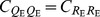
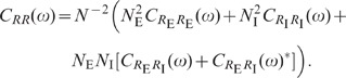
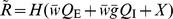
Population averaged correlations in cortical networks
The results presented in the previous subsections describe the fluctuations of
the compound activity. Pairwise correlations 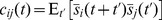 between the (centralized) spike trains
  are outside the scope of such a description. In this
subsection, we consider the same excitatory-inhibitory network as in
“
Results
: Population-activity fluctuations in
excitatory-inhibitory networks” and present a theory for the
population averaged spike-train cross-correlations. In general, this is a hard
problem. To understand the structure of cross-correlations, it is however
sufficient to derive a relationship between the cross- and auto-covariances in
the network, because the latter can, to good approximation, be understood in
mean-field theory. The integral of the auto-covariance function of spiking LIF
neurons can be calculated by Fokker-Planck formalism [12], [31], [51]. To determine the
relation between the cross-covariance and the auto-covariance, we replace the
spiking dynamics by a reduced linear model with covariances obeying, to linear
order, the same relation. We present the full derivation in
“
Methods
: Linearized network model”.
There, we first derive an approximate linear relation between the auto- and
cross-covariance functions
are outside the scope of such a description. In this
subsection, we consider the same excitatory-inhibitory network as in
“
Results
: Population-activity fluctuations in
excitatory-inhibitory networks” and present a theory for the
population averaged spike-train cross-correlations. In general, this is a hard
problem. To understand the structure of cross-correlations, it is however
sufficient to derive a relationship between the cross- and auto-covariances in
the network, because the latter can, to good approximation, be understood in
mean-field theory. The integral of the auto-covariance function of spiking LIF
neurons can be calculated by Fokker-Planck formalism [12], [31], [51]. To determine the
relation between the cross-covariance and the auto-covariance, we replace the
spiking dynamics by a reduced linear model with covariances obeying, to linear
order, the same relation. We present the full derivation in
“
Methods
: Linearized network model”.
There, we first derive an approximate linear relation between the auto- and
cross-covariance functions  and
and  , respectively, of
the LIF network. A direct solution of this equation is difficult. In the second
step, we therefore show that there exists a linear stochastic system with
activity
, respectively, of
the LIF network. A direct solution of this equation is difficult. In the second
step, we therefore show that there exists a linear stochastic system with
activity  and correlations
 and
and
 fulfilling the
same equation as the original LIF model. This reduced model can be solved in the
frequency domain by standard Fourier methods. Its solution allows us, by
construction, to determine the relation between the integral cross-covariances
fulfilling the
same equation as the original LIF model. This reduced model can be solved in the
frequency domain by standard Fourier methods. Its solution allows us, by
construction, to determine the relation between the integral cross-covariances
 and the integral
auto-covariances
and the integral
auto-covariances  up to linear
order.
up to linear
order.
As we are interested in the covariances averaged over many pairs of neurons, we
average the resulting set of  linear self-consistency equations (56) for the covariance matrix in the
frequency domain
linear self-consistency equations (56) for the covariance matrix in the
frequency domain  over statistically
identical pairs of neurons and many realizations of the random connectivity (see
“
Methods
: Population averaged correlations in the
linear EI network”). This yields a four-dimensional linear
system (76) describing the population averaged variances
over statistically
identical pairs of neurons and many realizations of the random connectivity (see
“
Methods
: Population averaged correlations in the
linear EI network”). This yields a four-dimensional linear
system (76) describing the population averaged variances  and
and  of the excitatory and inhibitory subpopulations, and the covariances
 and
and
 for unconnected
excitatory-excitatory and inhibitory-inhibitory neuron pairs, respectively (note
that we use the terms “variance” and “covariance” to
describe the integral of the auto- and cross-correlation
function, respectively; in many other studies, they refer to the zero-lag
correlation functions instead). The dependence of the variances and covariances
on the coupling strength
for unconnected
excitatory-excitatory and inhibitory-inhibitory neuron pairs, respectively (note
that we use the terms “variance” and “covariance” to
describe the integral of the auto- and cross-correlation
function, respectively; in many other studies, they refer to the zero-lag
correlation functions instead). The dependence of the variances and covariances
on the coupling strength  , obtained by
numerically solving (76), is shown in Fig. 6. We observe that the variances
, obtained by
numerically solving (76), is shown in Fig. 6. We observe that the variances
 and
and
 of excitatory and
inhibitory neurons are barely distinguishable (Fig. 6 A). With the approximation
of excitatory and
inhibitory neurons are barely distinguishable (Fig. 6 A). With the approximation
 , explicit
expressions can be obtained for the covariances (thick dashed curves Fig. 6 E):
, explicit
expressions can be obtained for the covariances (thick dashed curves Fig. 6 E):
Figure 6. Dependence of population averaged correlations and population-rate
fluctuations on the effective coupling  in a
linearized homogeneous network with excitatory-inhibitory
coupling.
in a
linearized homogeneous network with excitatory-inhibitory
coupling.

A: Spike-train variances  (black)
and
(black)
and  (gray) of
excitatory and inhibitory neurons. B: Spike-train
covariances
(gray) of
excitatory and inhibitory neurons. B: Spike-train
covariances  (black
solid),
(black
solid),  (dark gray
solid) and
(dark gray
solid) and  (light
gray solid) for excitatory-excitatory, excitatory-inhibitory and
inhibitory-inhibitory neuron pairs in the recurrent network,
respectively, and shared-input contribution
(light
gray solid) for excitatory-excitatory, excitatory-inhibitory and
inhibitory-inhibitory neuron pairs in the recurrent network,
respectively, and shared-input contribution  (black
dotted curve; ‘feedforward case’). C:
Decomposition of the total input covariance
(black
dotted curve; ‘feedforward case’). C:
Decomposition of the total input covariance  (light
gray) into shared-input covariance
(light
gray) into shared-input covariance  (black)
and weighted spike-train covariance
(black)
and weighted spike-train covariance  (dark
gray). Covariances in A, B and C are given in units of the noise
variance
(dark
gray). Covariances in A, B and C are given in units of the noise
variance  .
D: Input-correlation coefficient
.
D: Input-correlation coefficient  in the
recurrent network (black solid curve). In the feedforward case, the
input-correlation coefficient is identical to the network connectivity
in the
recurrent network (black solid curve). In the feedforward case, the
input-correlation coefficient is identical to the network connectivity
 (horizontal dotted line). E: Spike-train correlation
coefficients
(horizontal dotted line). E: Spike-train correlation
coefficients  (black),
 (dark
gray) and
(dark
gray) and  (solid
light gray curve) for excitatory-excitatory, excitatory-inhibitory and
inhibitory-inhibitory neuron pairs, respectively. Thick dashed curves
represent approximate solutions assuming
(solid
light gray curve) for excitatory-excitatory, excitatory-inhibitory and
inhibitory-inhibitory neuron pairs, respectively. Thick dashed curves
represent approximate solutions assuming  .
F: Low-frequency (LF) power ratios
.
F: Low-frequency (LF) power ratios  (black),
 (dark
gray),
(dark
gray),  (solid
light gray) for the population rate
(solid
light gray) for the population rate  and the
excitatory and inhibitory subpopulation rates
and the
excitatory and inhibitory subpopulation rates  and
and
 ,
respectively. The LF power ratio represents the ratio between the LF
spectra in the recurrent network and for the case where the feedback
channels are replaced by feedforward input with
,
respectively. The LF power ratio represents the ratio between the LF
spectra in the recurrent network and for the case where the feedback
channels are replaced by feedforward input with  (cf. Fig. 5 C). Thick
dashed curves in F show power ratios obtained by assuming that the
auto-correlations are identical in the feedback and the feedforward
scenario (see main text). Vertical dotted lines mark the stability limit
of the linear model (see “
Methods
: Linearized network
model”). A–F:
(cf. Fig. 5 C). Thick
dashed curves in F show power ratios obtained by assuming that the
auto-correlations are identical in the feedback and the feedforward
scenario (see main text). Vertical dotted lines mark the stability limit
of the linear model (see “
Methods
: Linearized network
model”). A–F:  ,
,
 ,
,
 ,
,
 ,
,
 ,
,
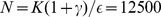 .
.
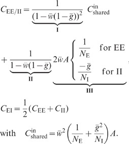 |
(19) |
The deviations from the full solutions (thin solid curves in Fig. 6 E), i.e. for  , are small. In the reduced model, both the external
input and the spiking of individual neurons contribute to an effective noise. As
the fluctuations in the reduced model depend linearly on the amplitude
, are small. In the reduced model, both the external
input and the spiking of individual neurons contribute to an effective noise. As
the fluctuations in the reduced model depend linearly on the amplitude
 of this noise, the
variances
of this noise, the
variances  and covariances
 (
( ) can be expressed in units of the noise variance
 . Consequently, the
correlation coefficients
. Consequently, the
correlation coefficients  are independent of
 (see Fig. 6).
The analytical form (19) of the result shows that the correlations are smaller
than expected given the amount of shared input a pair of neurons receives: The
quantity  in the first line
is the contribution of shared input to the covariance. For strong coupling
in the first line
is the contribution of shared input to the covariance. For strong coupling
 , the prefactor
 causes a
suppression of this contribution. Its structure is typical for a feedback
system, similar to the solution (3) of the one-population or the solution (52)
of the two-population model. The term
causes a
suppression of this contribution. Its structure is typical for a feedback
system, similar to the solution (3) of the one-population or the solution (52)
of the two-population model. The term  in the denominator represents the negative feedback of the compound rate. The
prefactor
in the denominator represents the negative feedback of the compound rate. The
prefactor  in the second line
of (19) is again due to the feedback and suppresses the contribution of the
factor
in the second line
of (19) is again due to the feedback and suppresses the contribution of the
factor  , which represents
the effect of direct connections between neurons.
, which represents
the effect of direct connections between neurons.
Our results are consistent with a previous study of the decorrelation mechanism:
In [17], the
authors considered how correlations scale with the size  of the network where the synaptic weights are chosen as
 . As a result, the
covariance
. As a result, the
covariance  in (19) caused by
shared input is independent of the network size, while the feedback
in (19) caused by
shared input is independent of the network size, while the feedback
 scales—to
leading order—as
scales—to
leading order—as  (see (45)).
Consequently, the first line in (19) scales as
(see (45)).
Consequently, the first line in (19) scales as  . The same scaling holds for the second line in (19),
explaining the decay of correlations as
. The same scaling holds for the second line in (19),
explaining the decay of correlations as  found in [17].
The first line in (19) is identical for any pair of neurons. The second line is
positive for a pair of excitatory neurons and negative for a pair of inhibitory
neurons. In other words, excitatory neurons are more correlated than inhibitory
ones. Together with the third line in (19), this reveals a characteristic
correlation structure: 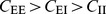 (Fig. 6 B,E). For strong
coupling
(Fig. 6 B,E). For strong
coupling  , the difference
between the excitatory and inhibitory covariance is
, the difference
between the excitatory and inhibitory covariance is 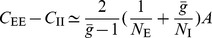 . The difference decreases as the level
  of inhibition is increased, i.e. the further the network
is in the inhibition dominated regime, away from the critical point
of inhibition is increased, i.e. the further the network
is in the inhibition dominated regime, away from the critical point
 .
.
To understand the suppression of shared-input correlations in recurrent
excitatory-inhibitory networks, consider the correlation between the local
inputs  of a pair of
neurons
of a pair of
neurons  ,
,  . The input-correlation coefficient
  can be expressed in terms of the averaged spike-train
covariances:
can be expressed in terms of the averaged spike-train
covariances:
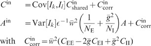 |
(20) |
(see “
Methods
: Population averaged correlations in the
linear EI network”: The input covariance  equals the average quantity
  given in (67), the input variance
  is given by (63) as
  ). The term
  represents the contribution due to the spike-train variances of the shared
presynaptic neurons (see (19)). This contribution is always positive (provided
the network architecture is consistent with Dale's law; see [15]). In a
purely feedforward scenario with uncorrelated presynaptic sources,
represents the contribution due to the spike-train variances of the shared
presynaptic neurons (see (19)). This contribution is always positive (provided
the network architecture is consistent with Dale's law; see [15]). In a
purely feedforward scenario with uncorrelated presynaptic sources,
 is the only
contribution to the input covariance of postsynaptic neurons. The resulting
response correlation for this feedforward case is much larger than in the
feedback system (Fig. 6 B,
black dotted curve). The correlation coefficient between inputs to a pair of
neurons in the feedforward case is identical to the network connectivity
is the only
contribution to the input covariance of postsynaptic neurons. The resulting
response correlation for this feedforward case is much larger than in the
feedback system (Fig. 6 B,
black dotted curve). The correlation coefficient between inputs to a pair of
neurons in the feedforward case is identical to the network connectivity
 (horizontal dotted
curve in Fig. 6 D; see [15]). In an
inhibition dominated recurrent network, spike-train correlations between pairs
of different source neurons contribute the additional term
(horizontal dotted
curve in Fig. 6 D; see [15]). In an
inhibition dominated recurrent network, spike-train correlations between pairs
of different source neurons contribute the additional term  , which is negative and of similar absolute value as the
shared-input contribution
, which is negative and of similar absolute value as the
shared-input contribution  . Thus, the two
terms
. Thus, the two
terms  and
and
 partly cancel each
other (see Fig. 6 C). In
consequence, the resulting input correlation coefficient
partly cancel each
other (see Fig. 6 C). In
consequence, the resulting input correlation coefficient  is smaller than
  (see Fig. 6 D; here:
 ).
).
The correlations in a purely inhibitory network can be obtained from (19) by
replacing  , taking into
account the negative sign of
, taking into
account the negative sign of  in
in  and setting
 and
and
 :
:
| (21) |
For finite coupling strength  ,
this expression is negative. The contributions of shared input and spike-train
correlations to the input correlation are given by
,
this expression is negative. The contributions of shared input and spike-train
correlations to the input correlation are given by 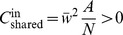 and
and  ,
respectively (see (19) and (20)). Using (21), we can directly verify that
,
respectively (see (19) and (20)). Using (21), we can directly verify that
 , because pairwise
correlations
, because pairwise
correlations  are negative,
leading to a partial cancellation
are negative,
leading to a partial cancellation 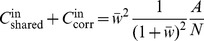 :
the right hand side is smaller in magnitude by a factor of
:
the right hand side is smaller in magnitude by a factor of  compared to each individual contribution. Hence, as in
the network with excitation and inhibition, shared-input correlations are partly
canceled by the contribution due to presynaptic pairwise spike-train
correlations. In the feedforward scenario with zero presynaptic spike-train
correlations, in contrast, the response correlations are determined by shared
input alone and are therefore increased. The suppression of shared-input
correlations in the feedback case is what we call ‘decorrelation’ in
the current work. In purely inhibitory networks, this decorrelation is caused by
weakly negative pairwise correlations (21). For sufficiently strong negative
feedback, correlations are smaller in absolute value as compared to the
feedforward case. The absolute value of these anti-correlations is bounded by
compared to each individual contribution. Hence, as in
the network with excitation and inhibition, shared-input correlations are partly
canceled by the contribution due to presynaptic pairwise spike-train
correlations. In the feedforward scenario with zero presynaptic spike-train
correlations, in contrast, the response correlations are determined by shared
input alone and are therefore increased. The suppression of shared-input
correlations in the feedback case is what we call ‘decorrelation’ in
the current work. In purely inhibitory networks, this decorrelation is caused by
weakly negative pairwise correlations (21). For sufficiently strong negative
feedback, correlations are smaller in absolute value as compared to the
feedforward case. The absolute value of these anti-correlations is bounded by
 .
.
The similarity in the results obtained for purely inhibitory networks and excitatory-inhibitory networks demonstrates that the suppression of pairwise correlations and population-activity fluctuations is a generic phenomenon in systems with negative feedback. It does not rely on an internal balance between excitation and inhibition.
As discussed in “
Results
: Suppression of population-rate
fluctuations in LIF networks”, the suppression of correlations
in the recurrent network is accompanied by a reduction of population-activity
fluctuations. With the population averaged correlations (19), the power (1) of
the population activity  reads
reads
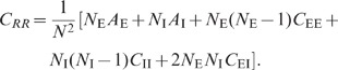 |
(22) |
In “
Results
: Population-activity fluctuations in
excitatory-inhibitory networks”, we showed that the
population-activity fluctuations are amplified if the local input in the
recurrent system is replaced by feedforward input from independent excitatory
and inhibitory populations (see Fig. 5 C). This manipulation corresponds to a neglect of
correlations  between excitatory
and inhibitory neurons. All remaining correlations (
between excitatory
and inhibitory neurons. All remaining correlations ( ,
,  ,
,  ,
,  ) are preserved.
With the resulting response auto- and cross-correlations
) are preserved.
With the resulting response auto- and cross-correlations  and
and  given by (84), the power (1) of the population activity becomes
| (23) |
For large effective coupling  ,
the power ratio
,
the power ratio  decays as
 (black curve in
Fig. 6 F). Note that the
power ratio
(black curve in
Fig. 6 F). Note that the
power ratio  derived here is
indistinguishable from the one we obtained in the framework of the population
model in “
Results
: Population-activity fluctuations in
excitatory-inhibitory networks” (black solid curve in Fig. 4 B). Although the
derivation of the macroscopic model in “
Results
: Population-activity fluctuations
in excitatory-inhibitory networks” is different from the one
leading to the population averaged correlations described here, the two models
are consistent: They describe one and the same system and lead to identical
power ratios.
derived here is
indistinguishable from the one we obtained in the framework of the population
model in “
Results
: Population-activity fluctuations in
excitatory-inhibitory networks” (black solid curve in Fig. 4 B). Although the
derivation of the macroscopic model in “
Results
: Population-activity fluctuations
in excitatory-inhibitory networks” is different from the one
leading to the population averaged correlations described here, the two models
are consistent: They describe one and the same system and lead to identical
power ratios.
The fluctuation suppression is not only observed at the level of the entire
network, i.e. for the population activity  ,
but also for each individual subpopulation
,
but also for each individual subpopulation  and
and  ,
i.e. for the subpopulation averaged activities
,
i.e. for the subpopulation averaged activities  and
and  .
The derivation of the corresponding power ratios
.
The derivation of the corresponding power ratios  and
and  is analog to the one described above. As a result of the correlation structure
 in the feedback
system (see Fig. 6 B), the
power of the inhibitory population activity is smaller than the power of the
excitatory population activity. In consequence,
in the feedback
system (see Fig. 6 B), the
power of the inhibitory population activity is smaller than the power of the
excitatory population activity. In consequence,  (gray curves in Fig. 6 F).
In (22) and (23), the auto-correlations are scaled by  , while the cross-correlations enter with a prefactor of
order unity. For large
, while the cross-correlations enter with a prefactor of
order unity. For large  , one may therefore
expect that the suppression of population-activity fluctuations is essentially
mediated by pairwise correlations. In the recurrent system, however, the
cross-correlations
, one may therefore
expect that the suppression of population-activity fluctuations is essentially
mediated by pairwise correlations. In the recurrent system, however, the
cross-correlations  (
( ) are of order
  (see Fig. 6 and (19)). It is
therefore a priori not clear whether the fluctuation suppression is indeed
dominated by pairwise correlations. In our framework, one can explicitly show
that the auto-correlation is irrelevant: Replacing the auto-correlation
(see Fig. 6 and (19)). It is
therefore a priori not clear whether the fluctuation suppression is indeed
dominated by pairwise correlations. In our framework, one can explicitly show
that the auto-correlation is irrelevant: Replacing the auto-correlation
 in (23) by the
average auto-correlation
in (23) by the
average auto-correlation 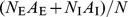 of the intact
feedback system has no visible effect on the resulting power ratio (dashed
curves in Fig. 6 F). The
difference in the spectra of the population activities
of the intact
feedback system has no visible effect on the resulting power ratio (dashed
curves in Fig. 6 F). The
difference in the spectra of the population activities  and
and  is therefore essentially caused by the cross-correlations.
The absolute population-activity fluctuations in purely inhibitory and in
excitatory-inhibitory networks show a qualitatively different dependence on the
synaptic coupling  , in agreement with
the previous sections. In networks with excitation and inhibition, the
correlation coefficient increases with increasing synaptic coupling (see Fig. 6 E). Hence, the
population-activity fluctuations grow with increasing coupling strength. In
purely inhibitory networks, in contrast, the pairwise spike-train correlation
decreases monotonously with increasing magnitude of the coupling strength
, in agreement with
the previous sections. In networks with excitation and inhibition, the
correlation coefficient increases with increasing synaptic coupling (see Fig. 6 E). Hence, the
population-activity fluctuations grow with increasing coupling strength. In
purely inhibitory networks, in contrast, the pairwise spike-train correlation
decreases monotonously with increasing magnitude of the coupling strength
 , see (21). In
consequence, the population-activity fluctuations decrease. The underlying
reason is that, in the inhibitory network, the power of the population activity
is directly proportional to the covariance of the input currents, which is
actively suppressed, as shown above. For excitatory-inhibitory networks, these
two quantities are not proportional (compare (20) and (1)) due to the different
synaptic weights appearing in the input covariance.
, see (21). In
consequence, the population-activity fluctuations decrease. The underlying
reason is that, in the inhibitory network, the power of the population activity
is directly proportional to the covariance of the input currents, which is
actively suppressed, as shown above. For excitatory-inhibitory networks, these
two quantities are not proportional (compare (20) and (1)) due to the different
synaptic weights appearing in the input covariance.
To compare our theory to simulations of spiking LIF networks, we need to
determine the effect of a synaptic input on the response activity of the neuron
model. To this end, we employ the Fokker-Planck theory of the LIF model (see
“
Methods
: Response kernel of the LIF
model”). In this context, the steady state of the recurrent
network is characterized by the mean  and the standard deviation
  of the total synaptic input. Both
  and
and  depend on the
steady-state firing rate in the network. The steady-state firing rate can be
determined in a self-consistent manner [12] as the fixed point of the
firing rate approximation (42). The approximation predicts the firing rate to
sufficient accuracy of about
depend on the
steady-state firing rate in the network. The steady-state firing rate can be
determined in a self-consistent manner [12] as the fixed point of the
firing rate approximation (42). The approximation predicts the firing rate to
sufficient accuracy of about  (see Fig. 7 A). We then
obtain an analytical expression of the low-frequency transfer which relates the
fluctuation
(see Fig. 7 A). We then
obtain an analytical expression of the low-frequency transfer which relates the
fluctuation 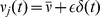 of a synaptic
input to neuron
of a synaptic
input to neuron  to the fluctuation
of neuron
to the fluctuation
of neuron  's response
firing rate to linear order, so that
's response
firing rate to linear order, so that 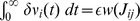 .
This relates the postsynaptic potential
.
This relates the postsynaptic potential  in the LIF model to the effective linear coupling
  in our linear theory. The functional relation
 can be derived in
analytical form by linearization of (42) about the steady-state working point.
Note that
can be derived in
analytical form by linearization of (42) about the steady-state working point.
Note that  depends on
 and
and
 and, hence, on the
steady-state firing rate in the network. The derivation outlined in
“
Methods
: Response kernel of the LIF
model” constitutes an extension of earlier work [21], [33] to
quadratic order in
and, hence, on the
steady-state firing rate in the network. The derivation outlined in
“
Methods
: Response kernel of the LIF
model” constitutes an extension of earlier work [21], [33] to
quadratic order in  . The results agree
well with those obtained by direct simulation for a large range of synaptic
amplitudes (see Fig. 8).
. The results agree
well with those obtained by direct simulation for a large range of synaptic
amplitudes (see Fig. 8).
Figure 7. Comparison between predictions of the linear theory (thick gray curves) and direct simulation of the LIF-network model (symbols and thin lines).

Dependence of the spike-train and population-rate statistics on the
synaptic weight  (PSP
amplitude) in a recurrent excitatory-inhibitory network (‘feedback
system’, ‘FB’) and in a population of unconnected
neurons receiving randomized feedforward input (‘feedforward
system’, ‘FF’) from neurons in the recurrent network.
Average presynaptic firing rates and shared-input structure are
identical in the two systems. In the FF case, the average correlations
between presynaptic spike-trains are homogenized (i.e.
(PSP
amplitude) in a recurrent excitatory-inhibitory network (‘feedback
system’, ‘FB’) and in a population of unconnected
neurons receiving randomized feedforward input (‘feedforward
system’, ‘FF’) from neurons in the recurrent network.
Average presynaptic firing rates and shared-input structure are
identical in the two systems. In the FF case, the average correlations
between presynaptic spike-trains are homogenized (i.e. 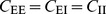 ) as a
result of the random reassignment of presynaptic neuron types. The
mapping of the LIF dynamics to the linear reduced dynamics
(“
Methods
: Response kernel of the LIF
model”) relates the PSP amplitude
) as a
result of the random reassignment of presynaptic neuron types. The
mapping of the LIF dynamics to the linear reduced dynamics
(“
Methods
: Response kernel of the LIF
model”) relates the PSP amplitude  to the
effective coupling strength
to the
effective coupling strength  by (45), as shown in Fig. 8 B. A: Average
firing rates
by (45), as shown in Fig. 8 B. A: Average
firing rates  in the FB
(black up-triangles: excitatory neurons; gray down-triangles: inhibitory
neurons) and in the FF system (open circles). Analytical prediction (??)
(gray curve). B: Spike-train correlation coefficients
in the FB
(black up-triangles: excitatory neurons; gray down-triangles: inhibitory
neurons) and in the FF system (open circles). Analytical prediction (??)
(gray curve). B: Spike-train correlation coefficients
 (black
up-triangles),
(black
up-triangles),  (gray
squares) and
(gray
squares) and  (gray
down-triangles) for excitatory-excitatory, excitatory-inhibitory, and
inhibitory-inhibitory neuron pairs, respectively, in the FB system.
Analytical prediction (19) (gray curves). Spike-train correlation
coefficient
(gray
down-triangles) for excitatory-excitatory, excitatory-inhibitory, and
inhibitory-inhibitory neuron pairs, respectively, in the FB system.
Analytical prediction (19) (gray curves). Spike-train correlation
coefficient  (open
circles) in the FF system with homogenized presynaptic spike-train
correlations. Analytical prediction (86) (underlying gray curve).
C: Shared-input (
(open
circles) in the FF system with homogenized presynaptic spike-train
correlations. Analytical prediction (86) (underlying gray curve).
C: Shared-input ( ; black up-triangles) and spike-correlation
contribution
; black up-triangles) and spike-correlation
contribution  (FB: gray
down-triangles; FF: open circles) to the input correlation
(FB: gray
down-triangles; FF: open circles) to the input correlation
 (normalized by
  ).
Analytical predictions (20). D: Low-frequency (LF) power
ratio of the compound activity. Vertical dotted lines in A–D mark
the stability limit of the linear model (see “
Methods
:
Linearized network model”).
).
Analytical predictions (20). D: Low-frequency (LF) power
ratio of the compound activity. Vertical dotted lines in A–D mark
the stability limit of the linear model (see “
Methods
:
Linearized network model”).  ,
,
 ,
,
 ,
,
 . Size of
postsynaptic population in the FF case:
. Size of
postsynaptic population in the FF case:  .
Simulation time:
.
Simulation time:  .
.
Figure 8. Linear response and relation between synaptic weight  and
effective coupling strength
and
effective coupling strength  .
.

A: Firing-rate deflection  of a LIF
neuron caused by an incoming spike event of postsynaptic amplitude
of a LIF
neuron caused by an incoming spike event of postsynaptic amplitude
 .
B: Integral
.
B: Integral 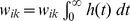 of the firing rate deflection shown in A as a
function of the postsynaptic amplitude
of the firing rate deflection shown in A as a
function of the postsynaptic amplitude  (simulation: black dots; analytical approximation (45) : gray curve).
The neuron receives constant synaptic background input with
(simulation: black dots; analytical approximation (45) : gray curve).
The neuron receives constant synaptic background input with
 ,
,
 , and rates
 ,
,
 resulting
in a first and second moment (42)
resulting
in a first and second moment (42)  and
and  . Simulation results are obtained by averaging
over
. Simulation results are obtained by averaging
over  trials of
 duration
each with
duration
each with  input
impulses on average. For further parameters of the neuron model, see
Table 1 and
Table 2.
input
impulses on average. For further parameters of the neuron model, see
Table 1 and
Table 2.
Fig. 7 B compares the
population averaged correlation coefficients  obtained from the linear reduced model, see (19), and
simulations of LIF networks. Note that the absolute value of the noise amplitude
obtained from the linear reduced model, see (19), and
simulations of LIF networks. Note that the absolute value of the noise amplitude
 in the reduced
model does not influence the correlation coefficient
in the reduced
model does not influence the correlation coefficient  , as both quantities
  and
and  depend linearly on
  . Theory and
simulation agree well for synaptic weights up to
. Theory and
simulation agree well for synaptic weights up to  . For larger synaptic amplitudes, the approximation of
the effective linear transfer for a single neuron obtained from the
Fokker-Planck theory deviates from its actual value (see Fig. 8 B). Fig. 7 C shows that the cancellation of the
input covariance in the LIF network is well explained by the theory.
. For larger synaptic amplitudes, the approximation of
the effective linear transfer for a single neuron obtained from the
Fokker-Planck theory deviates from its actual value (see Fig. 8 B). Fig. 7 C shows that the cancellation of the
input covariance in the LIF network is well explained by the theory.
Previous work [17] suggested that positive correlations between
excitatory and inhibitory inputs lead to a negative component in the input
correlation which, in turn, suppresses shared-input correlations. The mere
existence of positive correlations between excitatory and inhibitory inputs is
however not sufficient. To explain the effect, it is necessary to take the
particular correlation structure  into account. To illustrate this, consider the case where the correlation
structure is destroyed by replacing all pairwise correlations in the input
spike-train ensemble by the overall population average
into account. To illustrate this, consider the case where the correlation
structure is destroyed by replacing all pairwise correlations in the input
spike-train ensemble by the overall population average  (homogenization of correlations). The resulting response
correlations (upper gray curve in Fig. 7 B) are derived in “
Methods
: Population averaged correlations
in the linear EI network”, eq. (86). In simulations of LIF
networks, we study the effect of homogenized spike-train correlations by first
recording the activity of the intact recurrent network, randomly reassigning the
neuron type (
(homogenization of correlations). The resulting response
correlations (upper gray curve in Fig. 7 B) are derived in “
Methods
: Population averaged correlations
in the linear EI network”, eq. (86). In simulations of LIF
networks, we study the effect of homogenized spike-train correlations by first
recording the activity of the intact recurrent network, randomly reassigning the
neuron type ( or
or  ) to each recorded spike train, and feeding this activity
into a second population of neurons. Compared to the intact recurrent network,
the response correlations are significantly larger (Fig. 7 B). The contribution of homogenized
spike-train correlations to the input covariance
) to each recorded spike train, and feeding this activity
into a second population of neurons. Compared to the intact recurrent network,
the response correlations are significantly larger (Fig. 7 B). The contribution of homogenized
spike-train correlations to the input covariance  (see (20)) is given by
 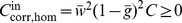 . For positive spike-train correlations
  , this contribution is greater or equal zero (zero for
 ). Hence, it cannot
compensate the (positive) shared-input contribution
). Hence, it cannot
compensate the (positive) shared-input contribution  (see Fig. 7
C). In consequence, input correlations, output correlations and, in
turn, population-rate fluctuations (Fig. 7 D) cannot be suppressed by homogeneous positive correlations
in the input spike-train ensemble. Canceling of shared-input correlations
requires either negative spike-train correlations (as in purely inhibitory
networks) or a heterogeneity in correlations across different pairs of neurons
(e.g.
(see Fig. 7
C). In consequence, input correlations, output correlations and, in
turn, population-rate fluctuations (Fig. 7 D) cannot be suppressed by homogeneous positive correlations
in the input spike-train ensemble. Canceling of shared-input correlations
requires either negative spike-train correlations (as in purely inhibitory
networks) or a heterogeneity in correlations across different pairs of neurons
(e.g.  ).
).
Effect of feedback manipulations
In the previous subsections, we quantified the suppression of population-rate fluctuations in recurrent networks by comparing the activity in the intact recurrent system (feedback scenario) to the case where the feedback is replaced by feedforward input with some predefined statistics (feedforward scenario). We particularly studied the effect of neglecting the auto-statistics of the compound feedback, (the structure of) correlations within the feedback ensemble and/or correlations between the feedback and the external input. In all cases, we observed a significant amplification of population-activity fluctuations in the feedforward scenario. In this subsection, we further investigate the role of different types of feedback manipulations by means of simulations of LIF networks with excitatory-inhibitory coupling. To this end, we record the spiking activity of the recurrent network (feedback case), apply different types of manipulations to this activity (described in detail below) and feed this modified activity into a second population of identical (unconnected) neurons (feedforward case). As before, the connectivity structure (in-degrees, shared-input structure, synaptic weights) is exactly identical in the feedback and the feedforward case.
In “
Methods
: Linearized network model”,
we show that the low-frequency fluctuations of the population rate
 of the spiking
model are captured by the reduced model
of the spiking
model are captured by the reduced model  presented in the previous subsections. To verify that the theory based on
excitatory and inhibitory population rates is indeed sufficient to explain the
decorrelation mechanism, we first consider the case where the sender identities
of the presynaptic spike train are randomly shuffled. Fig. 9 A shows the power-spectrum of the
population activity recorded in the original network (FB) as well as the spectra
obtained after shuffling spike-train identities within the excitatory and
inhibitory subpopulations separately (Shuff2D), or across the entire network
(Shuff1D). As shuffling of neuron identities does not change the population
rates, all three compound spectra are identical. Fig. 9 B shows the response power-spectra of
the neuron population receiving the shuffled spike trains. Shuffling within the
subpopulations (Shuff2D) preserves the population-specific fluctuations and
average correlations. The effect on the response fluctuations is negligible
(compare black and light gray curves in Fig. 9 B). In particular, the power of
low-frequency fluctuations remains unchanged (Fig. 9 C). This result confirms that
population models which take excitatory and inhibitory activity separately into
account are sufficient to explain the observations. Shuffling of spike-train
identities across subpopulations (Shuff1D), in contrast, causes an increase in
the population fluctuations by about one order of magnitude (Fig. 9 B,C; dark gray). This
outcome is in agreement with the result obtained by homogenizing pairwise
correlations (see Fig. 7)
and demonstrates that the excitatory and inhibitory subpopulation rates have to
be conserved to explain the observed fluctuation suppression.
presented in the previous subsections. To verify that the theory based on
excitatory and inhibitory population rates is indeed sufficient to explain the
decorrelation mechanism, we first consider the case where the sender identities
of the presynaptic spike train are randomly shuffled. Fig. 9 A shows the power-spectrum of the
population activity recorded in the original network (FB) as well as the spectra
obtained after shuffling spike-train identities within the excitatory and
inhibitory subpopulations separately (Shuff2D), or across the entire network
(Shuff1D). As shuffling of neuron identities does not change the population
rates, all three compound spectra are identical. Fig. 9 B shows the response power-spectra of
the neuron population receiving the shuffled spike trains. Shuffling within the
subpopulations (Shuff2D) preserves the population-specific fluctuations and
average correlations. The effect on the response fluctuations is negligible
(compare black and light gray curves in Fig. 9 B). In particular, the power of
low-frequency fluctuations remains unchanged (Fig. 9 C). This result confirms that
population models which take excitatory and inhibitory activity separately into
account are sufficient to explain the observations. Shuffling of spike-train
identities across subpopulations (Shuff1D), in contrast, causes an increase in
the population fluctuations by about one order of magnitude (Fig. 9 B,C; dark gray). This
outcome is in agreement with the result obtained by homogenizing pairwise
correlations (see Fig. 7)
and demonstrates that the excitatory and inhibitory subpopulation rates have to
be conserved to explain the observed fluctuation suppression.
Figure 9. Amplification of population-rate fluctuations by different types of feedback manipulations in a random network of excitatory and inhibitory LIF neurons (simulation results).

Top row (A–C): Unperturbed feedback (FB;
black), shuffling of spike-train senders across entire network (Shuff1D;
dark gray) and within each subpopulation (E,I) separately (Shuff2D;
light gray). Bottom row (D–F):
Unperturbed feedback (FB; black), replacement of spike trains by
realizations of inhomogeneous (PoissI; dark gray) and homogeneous
Poisson processes (PoissH; light gray). In the PoissI (PoissH) case, the
(time averaged) subpopulation rates are approximately preserved.
A, D: Compound power-spectra
 of input
spike-train ensembles. B, E: Power-spectra
of input
spike-train ensembles. B, E: Power-spectra
 of
population-response rates. C, F: Low-frequency
(LF;
of
population-response rates. C, F: Low-frequency
(LF;  –
– ) power ratio
  (increase
in LF power relative to the unperturbed case [FB]; logarithmic
scaling). Note that in A, the compound-input spectra (FB, Shuff1D,
Shuff2D) are identical. In D, the input spectra for the intact recurrent
network (FB) and the inhomogeneous-Poisson case (PoissI) are barely
distinguishable. See Table 1 and Table 2 for details on the network model and parameters.
Simulation time
(increase
in LF power relative to the unperturbed case [FB]; logarithmic
scaling). Note that in A, the compound-input spectra (FB, Shuff1D,
Shuff2D) are identical. In D, the input spectra for the intact recurrent
network (FB) and the inhomogeneous-Poisson case (PoissI) are barely
distinguishable. See Table 1 and Table 2 for details on the network model and parameters.
Simulation time  .
Single-trial spectra smoothed by moving average (frame size
.
Single-trial spectra smoothed by moving average (frame size
 ).
).
The shuffling experiments and the results of the linear model in the previous subsections suggest that the precise temporal structure of the population averaged activities within homogeneous subpopulations is essential for the suppression of population-rate fluctuations. Preserving the exact structure of individual spike trains is not required. This is confirmed by simulation experiments where new sender identities were randomly reassigned for each individual presynaptic spike (rather than for each spike train; data not shown). This operation destroys the structure of individual spike trains but preserves the compound activities. The results are similar to those reported here.
So far, it is unclear how sensitive the fluctuation-suppression mechanism is to
perturbations of the temporal structure of the population rates. To address this
question, we replaced the excitatory and inhibitory spike trains in the feedback
ensemble by independent realizations of inhomogeneous Poisson processes (PoissI)
with intensities given by the measured excitatory and inhibitory population
rates  and
and
 of the recurrent
network, respectively. Note that the compound rates of a single realization of
this new spike-train ensemble are similar but not identical to the original
population rates
of the recurrent
network, respectively. Note that the compound rates of a single realization of
this new spike-train ensemble are similar but not identical to the original
population rates  ,
,  (in each time window
  , the resulting spike count is a random number drawn from
a Poisson distribution with mean and variance proportional to
, the resulting spike count is a random number drawn from
a Poisson distribution with mean and variance proportional to  and
and  ,
respectively). Although the compound spectrum of the resulting local input is
barely distinguishable from the compound spectrum of the intact recurrent system
(Fig. 9 D; black and
dark gray curves), the response spectra are very different: replacing the
feedback ensemble by inhomogeneous Poisson processes leads to a substantial
amplification of low-frequency fluctuations (Fig. 9 E; compare black and dark gray
curves). The effect is as strong as if the temporal structure of the population
rates was completely ignored, i.e. if the feedback channels were replaced by
realizations of homogeneous Poisson processes with constant rates (PoissH; light
gray curves in Fig. 9 D,E).
This result indicates that the precise temporal structure of the population
rates is essential and that even small deviations can significantly weaken the
fluctuation-suppression mechanism. The results of the Poisson experiments can be
understood by considering the effect of the additional noise caused by the
stochastic realization of individual spikes. Considering the auto-correlation, a
Poisson spike-train ensemble with rate profile
,
respectively). Although the compound spectrum of the resulting local input is
barely distinguishable from the compound spectrum of the intact recurrent system
(Fig. 9 D; black and
dark gray curves), the response spectra are very different: replacing the
feedback ensemble by inhomogeneous Poisson processes leads to a substantial
amplification of low-frequency fluctuations (Fig. 9 E; compare black and dark gray
curves). The effect is as strong as if the temporal structure of the population
rates was completely ignored, i.e. if the feedback channels were replaced by
realizations of homogeneous Poisson processes with constant rates (PoissH; light
gray curves in Fig. 9 D,E).
This result indicates that the precise temporal structure of the population
rates is essential and that even small deviations can significantly weaken the
fluctuation-suppression mechanism. The results of the Poisson experiments can be
understood by considering the effect of the additional noise caused by the
stochastic realization of individual spikes. Considering the auto-correlation, a
Poisson spike-train ensemble with rate profile  is equivalent to a sum of the rate profile and a noise
term resulting from the stochastic (Poissonian) realization of spikes,
is equivalent to a sum of the rate profile and a noise
term resulting from the stochastic (Poissonian) realization of spikes,
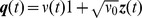 . Here,
 denotes a Gaussian
white noise with auto-correlation
denotes a Gaussian
white noise with auto-correlation 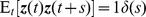 and
and  the mean firing
rate. The response fluctuations of the population driven by the rate modulated
Poisson activity are, to linear approximation, given by
the mean firing
rate. The response fluctuations of the population driven by the rate modulated
Poisson activity are, to linear approximation, given by  . Inserting
  ,
we obtain an additional noise term
,
we obtain an additional noise term  in the spectrum
  which explains the
increase in power compared to the spectrum
which explains the
increase in power compared to the spectrum  of the recurrent network. As a generalization of the
Poisson model, one may replace the noise amplitude
of the recurrent network. As a generalization of the
Poisson model, one may replace the noise amplitude  by some arbitrary prefactor
  . In simulation experiments, we observed a gradual
amplification of the population-rate fluctuations with increasing noise
amplitude
. In simulation experiments, we observed a gradual
amplification of the population-rate fluctuations with increasing noise
amplitude  (data not
shown).
(data not
shown).
Discussion
We have shown that negative feedback in recurrent neural networks actively suppresses low-frequency fluctuations of the population activity and pairwise correlations. This mechanism allows neurons to fire more independently than expected given the amount of shared presynaptic input. We demonstrated that manipulations of the feedback statistics, e.g. replacing feedback by uncorrelated feedforward input, can lead to a significant amplification of response correlations and population-rate fluctuations.
The suppression of correlations and population-rate fluctuations by feedback can be
observed in networks with both purely inhibitory and mixed excitatory-inhibitory
coupling. In purely inhibitory networks, the effect can be understood by studying
the role of the effective negative feedback experienced by the compound activity. In
networks of excitatory and inhibitory neurons, a change of coordinates, technically
a Schur decomposition, exposes the underlying feedback structure: the sum of the
excitatory and inhibitory activity couples negatively to itself if the network is in
an inhibition dominated regime (which is required for its stability; see, e.g.,
[12). This negative feedback suppresses fluctuations in a similar way as in
purely inhibitory networks. The fluctuation suppression becomes more efficient the
further the network is brought into the inhibition dominated regime, away from the
critical point of equal recurrent excitation and inhibition ( ). Having identified negative feedback as the underlying
cause of small fluctuations and correlations, we can rule out previous explanations
based on a balance between (correlated) excitation and inhibition [17]. We presented a
self-consistent theory for the average pairwise spike-train correlations which
illuminates that the suppression of population-rate fluctuations and the suppression
of pairwise correlations are two expressions of the same effect: as the single
spike-train auto-covariance is the same in the feedforward and the feedback case,
the suppression of population-rate fluctuations implies smaller correlations. Our
theory enables us to identify the cancellation of input correlations as a hallmark
of small spike-train correlations.
). Having identified negative feedback as the underlying
cause of small fluctuations and correlations, we can rule out previous explanations
based on a balance between (correlated) excitation and inhibition [17]. We presented a
self-consistent theory for the average pairwise spike-train correlations which
illuminates that the suppression of population-rate fluctuations and the suppression
of pairwise correlations are two expressions of the same effect: as the single
spike-train auto-covariance is the same in the feedforward and the feedback case,
the suppression of population-rate fluctuations implies smaller correlations. Our
theory enables us to identify the cancellation of input correlations as a hallmark
of small spike-train correlations.
In previous studies, shared presynaptic input has often been considered a main source
of correlation in recurrent networks (e.g. [15], [52]). Recently [17], suspected that
correlations between excitatory and inhibitory neurons and the fast tracking of
external input by the excitatory and the inhibitory population are responsible for
an active decorrelation. We have demonstrated here that the mere fact that
excitatory and inhibitory neurons are correlated is not sufficient to suppress
shared-input correlations. Rather, we find that the spike-train correlation
structure in networks of excitatory and inhibitory networks arranges such that their
overall contribution to the covariance between the summed inputs to a pair of
neurons becomes negative, canceling partly the effect of shared inputs. This
cancellation becomes more precise the stronger the negative compound feedback
 is. In homogeneous
networks where excitatory and inhibitory neurons receive statistically identical
input, the particular structure of correlations is
is. In homogeneous
networks where excitatory and inhibitory neurons receive statistically identical
input, the particular structure of correlations is  . It can further be shown that this structure of correlations
is preserved in the limit of large networks
. It can further be shown that this structure of correlations
is preserved in the limit of large networks  (
( ). For non-homogeneous
synaptic connectivity, if the synaptic amplitudes depend on the type of the target
neuron (i.e.
). For non-homogeneous
synaptic connectivity, if the synaptic amplitudes depend on the type of the target
neuron (i.e.  or
or  ), the structure of correlations may be different. Still, the
correlation structure arranges such that shared input correlation is effectively
suppressed. Formally, this can be seen from a self-consistency equation similar to
our equation (80).
), the structure of correlations may be different. Still, the
correlation structure arranges such that shared input correlation is effectively
suppressed. Formally, this can be seen from a self-consistency equation similar to
our equation (80).
The study by [17]
has shown that correlations are suppressed in the limit of infinitely large networks
of binary neurons receiving randomly drawn inputs from a common external population.
Its argument rests on the insight that the population-activity fluctuations in a
recurrent balanced network follow the fluctuations of the external common
population. An elegant scaling consideration for infinitely large networks
 with vanishing
synaptic efficacy
with vanishing
synaptic efficacy  shows that this fast
tracking becomes perfect in the limit. This allows to determine the zero-lag
pairwise correlations caused by the external input. The analysis methods and the
recurrent networks presented here differ in several respects from these previous
results: We study networks of a finite number of spiking model neurons. The neurons
receive uncorrelated external input, so that correlations are due to the local
recurrent connectivity among neurons, not due to tracking of the common external
input [17].
Moreover, we consider homogeneous connectivity where synaptic weights depend only on
the type of the presynaptic neuron (as, e.g., in [12]), resulting in a correlation
structure
shows that this fast
tracking becomes perfect in the limit. This allows to determine the zero-lag
pairwise correlations caused by the external input. The analysis methods and the
recurrent networks presented here differ in several respects from these previous
results: We study networks of a finite number of spiking model neurons. The neurons
receive uncorrelated external input, so that correlations are due to the local
recurrent connectivity among neurons, not due to tracking of the common external
input [17].
Moreover, we consider homogeneous connectivity where synaptic weights depend only on
the type of the presynaptic neuron (as, e.g., in [12]), resulting in a correlation
structure  . For such
connectivity, networks of binary neurons with uncorrelated external input exhibit
qualitatively the same correlation structure as reported here (results not
shown).
. For such
connectivity, networks of binary neurons with uncorrelated external input exhibit
qualitatively the same correlation structure as reported here (results not
shown).
In purely inhibitory networks, the decorrelation occurs in an analog manner as in
excitatory-inhibitory networks. As only a single population of neurons is available
here, population averaged spike-train correlations  are negative. This negative contribution compensates the
positive contribution of shared input.
are negative. This negative contribution compensates the
positive contribution of shared input.
The structure of integrated spike-train covariances in networks constitutes an
experimentally testable prediction. Note, however, that the prediction (19) obtained
in the current work rests on two simplifying assumptions: identical internal
dynamics of excitatory and inhibitory neurons and homogeneous connectivity (i.e.
 ,
,  ; see “
Results
: Population-activity fluctuations in
excitatory-inhibitory networks”). For such networks, the structure
of correlations is given by
; see “
Results
: Population-activity fluctuations in
excitatory-inhibitory networks”). For such networks, the structure
of correlations is given by  . Further, the relation
between subthreshold membrane-potential fluctuations and spike responses is the same
for both neuron types. Consequently, the above correlation structure can be observed
not only at the level of spike trains but also for membrane potentials, provided the
assumptions hold true. A recent experimental study [53] reports neuron-type specific
cross-correlation functions in the barrel cortex of behaving mice, both for spike
trains and membrane potentials. It is however difficult to assess the integral
correlations from the published data. A direct test of our predictions requires
either a reanalysis of the data or a theory predicting the entire correlation
functions. The raw (unnormalized) II and EI spike-train correlations in [53] are much more
pronounced than the EE correlations (Fig. 6 in [53]). This seems to be in contradiction to our results. Note,
however, that the firing rates of excitatory and inhibitory neurons are very
different in [53].
In our study, in contrast, the average firing rates of excitatory and inhibitory
neurons are identical as a consequence of the assumed network homogeneity. Future
theoretical work is needed to generalize our model to networks with heterogeneous
firing rates and non-homogeneous connectivity. Recent results on the dependence of
the correlation structure on the connectivity may prove useful in this endeavor
[54]–[56].
. Further, the relation
between subthreshold membrane-potential fluctuations and spike responses is the same
for both neuron types. Consequently, the above correlation structure can be observed
not only at the level of spike trains but also for membrane potentials, provided the
assumptions hold true. A recent experimental study [53] reports neuron-type specific
cross-correlation functions in the barrel cortex of behaving mice, both for spike
trains and membrane potentials. It is however difficult to assess the integral
correlations from the published data. A direct test of our predictions requires
either a reanalysis of the data or a theory predicting the entire correlation
functions. The raw (unnormalized) II and EI spike-train correlations in [53] are much more
pronounced than the EE correlations (Fig. 6 in [53]). This seems to be in contradiction to our results. Note,
however, that the firing rates of excitatory and inhibitory neurons are very
different in [53].
In our study, in contrast, the average firing rates of excitatory and inhibitory
neurons are identical as a consequence of the assumed network homogeneity. Future
theoretical work is needed to generalize our model to networks with heterogeneous
firing rates and non-homogeneous connectivity. Recent results on the dependence of
the correlation structure on the connectivity may prove useful in this endeavor
[54]–[56].
Correlations in spike-train ensembles play a crucial role for the en- and decoding of information. A set of uncorrelated spike trains provides a rich dynamical basis which allows readout neurons to generate a variety of responses by tuning the strength and filter properties of their synapses [1]
In the presence of correlations, the number of possible readout signals is limited.
Moreover, spike-train correlations impair the precision of such readout signals in
the presence of noise. Consider, for example, a linear combination 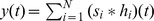 of
of  presynaptic spike
trains with arbitrary (linear) filter kernels
presynaptic spike
trains with arbitrary (linear) filter kernels  (e.g.
synaptic filters). In a realistic scenario, the individual spike trains
(e.g.
synaptic filters). In a realistic scenario, the individual spike trains
 typically vary across
trials [3], [57]. To understand
how robust the resulting readout signal
typically vary across
trials [3], [57]. To understand
how robust the resulting readout signal  is
against this spike-train variability, let's consider the variability of its
Fourier transform
is
against this spike-train variability, let's consider the variability of its
Fourier transform  . Assuming homogeneous
spike-train statistics,
. Assuming homogeneous
spike-train statistics,
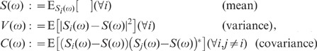 |
(24) |
the (squared) signal-to-noise ratio of the readout signal  is given by
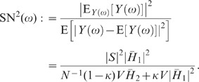 |
(25) |
Here,  denotes the average
across the ensemble of spike-train realizations,
denotes the average
across the ensemble of spike-train realizations, 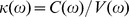 the spike-train coherence, and the coefficients
 and
and  the 1st- and 2nd-order filter statistics. For uncorrelated
spike trains, i.e.
the 1st- and 2nd-order filter statistics. For uncorrelated
spike trains, i.e.  , and
, and  , the signal-to-noise ratio
  grows unbounded with the population size
  . Thus, even for noisy spike trains (
 ), the compound signal
  can
be highly reliable if the population size
can
be highly reliable if the population size  is
sufficiently large. In the presence of correlations,
is
sufficiently large. In the presence of correlations,  , however,
  converges towards a constant value
  as
as
 grows. Even for large
populations, the readout signal remains prone to noise. These findings constitute a
generalization of the results reported for population-rate coding, i.e. sums of
unweighted spike counts (see, e.g., [2], [3]). The above arguments illustrate that the same reasoning
applies to coding schemes which are based on the spatio-temporal structure of spike
patterns.
grows. Even for large
populations, the readout signal remains prone to noise. These findings constitute a
generalization of the results reported for population-rate coding, i.e. sums of
unweighted spike counts (see, e.g., [2], [3]). The above arguments illustrate that the same reasoning
applies to coding schemes which are based on the spatio-temporal structure of spike
patterns.
In a previous study [9], we demonstrated that active decorrelation in recurrent networks is a necessary prerequisite for a controlled propagation of synchronous volleys of spikes in embedded feedforward subnetworks (‘synfire chains’; Fig. 10): A synfire chain receiving background input from a finite population of independent Poisson sources amplifies the resulting shared-input correlations, thereby leading to spontaneous synchronization within the chain (Fig. 10 B). A distinction between these spurious synchronous events and those triggered by an external stimulus is impossible. The synfire chain loses its asynchronous ground state [58]. A synfire chain receiving background inputs from a recurrent network, in contrast, is much more robust. Here, shared-input correlations are actively suppressed by the recurrent-network dynamics. Synchronous events can be triggered by external stimuli in a controlled manner (Fig. 10 A). Apart from the spontaneous synchronization illustrated in Fig. 10, decorrelation by inhibition might solve another problem arising in embedded synfire structures: In the presence of feedback connections between the synfire chain and the embedding background network, synchronous spike volleys can excite (high-frequency) oscillatory modes in the background network which, in turn, interfere with the synfire dynamics and prevent a robust propagation of synchronous activity within the chain (‘synfire explosion’; see [59], [60]). The decorrelation mechanism we refer to in our work is efficient only at low frequencies. It cannot prevent the build-up of these oscillations. [61] demonstrated that the ‘synfire explosion’ can be suppressed by adding inhibitory neurons to each synfire layer (‘shadow inhibition’) which diffusely project to neurons in the embedding network, thereby weakening the impact of synfire activity on the embedding network.
Figure 10. Recurrent network dynamics stabilizes dynamics of embedded synfire chains.

Spiking activity in a synfire chain ( layers, layer width
  ) receiving
background input from an excitatory-inhibitory network (A, cf.
Fig. 1 C) or from a
finite pool of excitatory and inhibitory Poisson processes (B,
cf. Fig. 1 D). Average
input firing rates, in-degrees and amount of shared input are identical in
both cases. Neurons of the first synfire layer (neuron ids
) receiving
background input from an excitatory-inhibitory network (A, cf.
Fig. 1 C) or from a
finite pool of excitatory and inhibitory Poisson processes (B,
cf. Fig. 1 D). Average
input firing rates, in-degrees and amount of shared input are identical in
both cases. Neurons of the first synfire layer (neuron ids  ) are
stimulated by current pulses at times
) are
stimulated by current pulses at times  and
and  . Each neuron in layer
  receives
inputs from all
receives
inputs from all  neurons in the
preceding layer
neurons in the
preceding layer  (synaptic
weights
(synaptic
weights  , spike
transmission delays
, spike
transmission delays  ), and
 and
and
 excitatory and
inhibitory background inputs, respectively, randomly drawn from the
presynaptic populations. Neurons in the first layer
excitatory and
inhibitory background inputs, respectively, randomly drawn from the
presynaptic populations. Neurons in the first layer  receive
 and
and
 excitatory and
inhibitory background inputs, respectively. Note that there is no feedback
from the synfire chain to the embedding network. See Table 2 for network parameters.
excitatory and
inhibitory background inputs, respectively. Note that there is no feedback
from the synfire chain to the embedding network. See Table 2 for network parameters.
In the present work we focus on the integral of the correlation function, nurtured by
our interest in the low-frequency fluctuations. An analog treatment can however
easily be performed for the zero-lag correlations. In contrast to infinite networks
with sparse connectivity ( ,
,  ), in the case of finite networks, pairs of neurons must be
distinguished according to whether they are synaptically connected or not in order
to arrive at a self-consistent theory for the averaged correlations. Providing
explicit expressions for correlations between connected and unconnected neurons, the
current work provides the tools to relate experimentally observed spiking
correlations to the underlying synaptic connectivity.
), in the case of finite networks, pairs of neurons must be
distinguished according to whether they are synaptically connected or not in order
to arrive at a self-consistent theory for the averaged correlations. Providing
explicit expressions for correlations between connected and unconnected neurons, the
current work provides the tools to relate experimentally observed spiking
correlations to the underlying synaptic connectivity.
The quantification of pairwise correlations is a necessary prerequisite to understand
how correlation sensitive synaptic plasticity rules, like spike-timing dependent
plasticity [62],
interact with the recurrent network dynamics [63]. Existing theories quantifying
correlations employ stochastic neuron models and are limited to purely excitatory
networks [63]–[65]. Here, we provide an analytical equivalence relation
between a reduced linear model and spiking integrate-and-fire neurons describing
fluctuations correctly up to linear order. A formally similar approach has been
employed earlier to study delayed cumulative inhibition in spiking networks [66]. We show that
the correlations observed in recurrent networks in the asynchronous irregular regime
are quantitatively captured for realistic synaptic coupling with postsynaptic
potentials of up to about  . The success of this
approach can be explained by the linearization of the neural threshold units by the
afferent noise experienced in the asynchronous regime. For linear neural dynamics,
the second-order description of fluctuations is closed [67]. We exploit this finding by
applying perturbation theory to the Fokker-Planck description of the
integrate-and-fire neuron to obtain the linear input-output transfer at low
frequencies [33],
thereby determining the effective coupling in our linear model.
. The success of this
approach can be explained by the linearization of the neural threshold units by the
afferent noise experienced in the asynchronous regime. For linear neural dynamics,
the second-order description of fluctuations is closed [67]. We exploit this finding by
applying perturbation theory to the Fokker-Planck description of the
integrate-and-fire neuron to obtain the linear input-output transfer at low
frequencies [33],
thereby determining the effective coupling in our linear model.
The scope of the theory presented in the current work is limited mainly by three
assumptions. The first is the use of a linear theory which exhibits an instability
as soon as a single eigenvalue of the effective connectivity matrix assumes a
positive real part. This ultimately happens when increasing the synaptic coupling
strength, because the eigenvalues of the random connectivity matrix are located in a
circle centered in the left half of the complex plain with a radius given by the
square root of the variance of the matrix elements [68], [69]. Nonlinearities, like those
imposed by strictly positive firing rates, prevent such unbounded growth (or decay)
by saturation. For nonlinear rate models with sigmoidal transfer functions it has
been shown that the activity of recurrent random networks of such units makes a
transition to chaos at the point where the linearized dynamics would loose stability
[70].
However, this point of transition is sharp only in the limit of infinitely large
networks. From the population averaged firing rate and the pairwise correlations
averaged over pairs of neurons considered in Fig. 7 we cannot conclude whether or not a
transition to chaos occurs in the spiking network. In simulations and in the
linearized reduced model, we could however observe that the distribution of pairwise
correlations broadens when approaching the point of instability. Future work needs
to examine this question in detail, e.g. by considering measures related to the
Lyapunov exponent. Recently developed semi-analytical theories accounting for
nonlinear neural features [71] may be helpful to answer this question. The second
limiting factor of the current theory is the use of a perturbative approach to
quantify the response of the integrate-and-fire model. Although the steady-state
firing rate of the network is found as the fixed point of the nonlinear
self-consistency equation, the response to a synaptic fluctuation is determined up
to linear order in the amplitude of the afferent rate fluctuation, which is only
valid for sufficiently small fluctuations. For larger input fluctuations, nonlinear
contributions to the neural response can become more important [33]. Also for strong synaptic
coupling, deviations from our theory are to be expected. Thirdly, the employment of
Fokker-Planck theory to determine the steady-state firing rate and the response to
incoming fluctuations assumes uncorrelated presynaptic firing with Poisson
statistics and synaptic amplitudes which are vanishingly small compared to the
distance between reset and threshold. For larger synaptic amplitudes, the
Fokker-Planck theory becomes approximate and deviations are expected [33], [34], [72], [73]. This can be
observed in Fig. 7 A, showing a
deviation between the self-consistent firing rate and the analytical prediction at
about  . In this work, we
obtained a sufficiently precise self-consistent approximation of the correlation
coefficient
. In this work, we
obtained a sufficiently precise self-consistent approximation of the correlation
coefficient  by relating the random
recurrent network of spiking neurons in the asynchronous irregular state to a
reduced linear model which obeys the same relation between
by relating the random
recurrent network of spiking neurons in the asynchronous irregular state to a
reduced linear model which obeys the same relation between  and
and  up to linear order.
This reduced linear model, however, does not predict the absolute values of the
variance
up to linear order.
This reduced linear model, however, does not predict the absolute values of the
variance  and covariance
 . The variance
 of the LIF model, for
example, is dominated by nonlinear effects, such as the reset mechanism after each
action potential. Previous work [12], [31] has shown that the single spike-train statistics can be
approximated in the diffusion approximation if the recurrent firing rate in the
network is determined by mean-field theory. One may therefore extend our approach
and determine the integral auto-correlation function as
of the LIF model, for
example, is dominated by nonlinear effects, such as the reset mechanism after each
action potential. Previous work [12], [31] has shown that the single spike-train statistics can be
approximated in the diffusion approximation if the recurrent firing rate in the
network is determined by mean-field theory. One may therefore extend our approach
and determine the integral auto-correlation function as  with the Fano factor
  (see
[51]). For
a renewal process and long observation times, the Fano factor is given by
(see
[51]). For
a renewal process and long observation times, the Fano factor is given by
 [74], [75]. The
coefficient of variation
[74], [75]. The
coefficient of variation  can be obtained from
the diffusion approximation of the membrane-potential dynamics (App. A.1 in
[12). The covariance
can be obtained from
the diffusion approximation of the membrane-potential dynamics (App. A.1 in
[12). The covariance  can then be determined
by (19). Another possibility is the use of a refractory-density approach [76], [77].
can then be determined
by (19). Another possibility is the use of a refractory-density approach [76], [77].
The spike-train correlation as a function of the time lag is an experimentally accessible measure. Future theoretical work should therefore also focus on the temporal structure of correlations in recurrent networks, going beyond zero-lag correlations [15], [17] and the integral measures studied in the current work. This would allow to compare the theoretical predictions to direct experimental observations in a more detailed manner. Moreover, the relative spike timing between pairs of neurons is a decisive property for Hebbian learning [78] in recurrent networks, as implemented by spike timing-dependent plasticity [62], and suspected to play a role for synapse formation and elimination [79].
The simulation experiments performed in this work revealed that the suppression of correlations is vulnerable to certain types of manipulations of the feedback loop. One particular biological source of additional variability in the feedback loop is probabilistic vesicle release at synapses [80]. In feedforward networks, such unreliable synaptic transmission has been shown to decrease the transmission of correlations by pairs of neurons [22]. Stochastic synaptic release is very similar to the replacement of the population activity in the feedback branch by a rate modulated Poisson processes that conserves the population rate. In these simulations we observed an increase of correlations due to the additional noise caused by the stochastic Poisson realization. Future work should investigate more carefully which of the two opposing effects of probabilistic release on correlations dominates in recurrent networks.
The results of our study do not only shed light on the decorrelation of spiking
activity in recurrent neural networks. They also demonstrate that a standard
modeling approach in theoretical neuroscience is problematic: When studying the
dynamics of a local neural network (e.g. a “cortical column”), it is a
common strategy to replace external inputs to this neural population  by spike-train ensembles with some predefined statistics,
e.g. by stationary Poisson processes. Most neural systems, however, exhibit a high
degree of recurrence. Nonlocal input to the population
by spike-train ensembles with some predefined statistics,
e.g. by stationary Poisson processes. Most neural systems, however, exhibit a high
degree of recurrence. Nonlocal input to the population  , i.e. input from other brain areas, therefore has to be
expected to be shaped by the activity within
, i.e. input from other brain areas, therefore has to be
expected to be shaped by the activity within  . The
omission of these feedback loops can lead to qualitatively wrong predictions of the
population statistics. The analytical results for the correlation structure of
recurrent networks presented in this study provide the means to a more realistic
specification of such external activity.
. The
omission of these feedback loops can lead to qualitatively wrong predictions of the
population statistics. The analytical results for the correlation structure of
recurrent networks presented in this study provide the means to a more realistic
specification of such external activity.
Methods
LIF network model
In the present study, we consider two types of sparsely connected random networks: networks with purely inhibitory coupling (“I networks”) and networks with both excitatory and inhibitory interactions (“EI networks”). To illustrate the main findings of this study and to test the predictions of the linear model described in “ Methods : Linearized network model”, both architectures were implemented as networks of leaky integrate-and-fire (LIF) neurons. The model details and parameters are reported in Table 1 and Table 2, respectively. All network simulations were carried out with NEST (www.nest-initiative.org, [81]).
Table 1. LIF network: Model overview.
| A Model summary | |
| Populations | one (inhibitory network) or two (excitatory-inhibitory network) |
| Connectivity | random, fixed in-degrees |
| Neuron | leaky integrate-and-fire (LIF) |
| Synapse | current based, delta-shaped postsyn. currents with constant amplitudes |
| Input | uncorrelated Gaussian white noise currents |
Table 2. LIF network: Parameters (default values).
| A Connectivity | ||
| Name | Value | Description |

|
 (inhibitory network) (inhibitory network) |
in-degree |
 (E-I network) (E-I network) |
excitatory in-degree | |

|

|
network connectivity |

|
 (E-I network) (E-I network) |
relative size of inhibitory subpopulation |
Linearized network model
In this section we show how the dynamics of the spiking network can be reduced to an effective linear model with fluctuations fulfilling, by construction, the same relationship as the original system up to linear order. We first outline the conceptual steps of this reduction, and then provide the formal derivation.
We make use of the observation that the effect of a single synaptic impulse on
the output activity of a neuron is typically small. Writing the response spike
train of a neuron as a functional of the history of all incoming impulses
therefore allows us to perform a linearization with respect to each of the
afferent spike trains. Formally, this corresponds to a Volterra expansion up to
linear order, the generalization of a Taylor series to functionals. In
“
Methods
: Response kernel of the LIF
model”, we perform this linearization explicitly for the
example of the LIF model. This determines how the linear response kernel depends
on the parameters of the LIF model. The linear dependence on the input leads to
an approximate convolution equation (31) linearly connecting the auto- and the
cross-correlation functions in the network. As this equation is complicated to
solve directly, we introduce a reduced linear model (35) obeying the same
convolution equation. The reduced linear model can be solved by standard Fourier
methods and yields an explicit form for the covariance matrix in the frequency
domain (37). The diagonal and off-diagonal elements of the  dimensional covariance matrix
  in (56) correspond to the power-spectra of individual
neurons and the cross-spectra of individual neuron pairs, respectively. As, in
this linear approximation, both the auto- and the cross-covariances are
proportional to the variance of the driving noise, the resulting correlation
coefficients are independent of the noise amplitude (see
“
Methods
: Population averaged correlations in the
linear EI network”). As shown in “
Results
: Suppression of
population-activity fluctuations by negative feedback” and
“
Results
: Population-activity fluctuations in
excitatory-inhibitory networks”, the suppression of
fluctuations in recurrent networks is most pronounced at low frequencies. It is
therefore sufficient to restrict the discussion to the zero-frequency limit
in (56) correspond to the power-spectra of individual
neurons and the cross-spectra of individual neuron pairs, respectively. As, in
this linear approximation, both the auto- and the cross-covariances are
proportional to the variance of the driving noise, the resulting correlation
coefficients are independent of the noise amplitude (see
“
Methods
: Population averaged correlations in the
linear EI network”). As shown in “
Results
: Suppression of
population-activity fluctuations by negative feedback” and
“
Results
: Population-activity fluctuations in
excitatory-inhibitory networks”, the suppression of
fluctuations in recurrent networks is most pronounced at low frequencies. It is
therefore sufficient to restrict the discussion to the zero-frequency limit
 . Note that the
zero-frequency variances and covariances correspond to the integrals of the
auto- and cross-correlation functions in the time domain. In this limit, we may
combine the two different sources of fluctuations caused by the spiking of the
neurons and by external input to the network into a single source of white noise
with variance
. Note that the
zero-frequency variances and covariances correspond to the integrals of the
auto- and cross-correlation functions in the time domain. In this limit, we may
combine the two different sources of fluctuations caused by the spiking of the
neurons and by external input to the network into a single source of white noise
with variance  (see (39)).
In general, the spiking activity  of neuron
  at time
 is determined by
the entire history
is determined by
the entire history  of the activity of
all neurons
of the activity of
all neurons  in the network up
to time
in the network up
to time  . Formally, this
dependence can be expressed by a functional
. Formally, this
dependence can be expressed by a functional
| (26) |
The subscript  in
in  indicates that
  (causality). In the following, we use the abbreviation
  . The effect of a single synaptic input on the state of a
neuron is typically small. We therefore approximate the influence of an incoming
spike train on the activity of the target neuron up to linear order. The
sensitivity of neuron
. The effect of a single synaptic input on the state of a
neuron is typically small. We therefore approximate the influence of an incoming
spike train on the activity of the target neuron up to linear order. The
sensitivity of neuron  's activity to
the input from neuron
's activity to
the input from neuron  can be expressed
by the functional derivative of
can be expressed
by the functional derivative of  with respect to input spike train
  :
:
| (27) |
It represents the response of the functional to a single  -shaped perturbation in input channel
  at time
  ,
normalized by the perturbation amplitude
,
normalized by the perturbation amplitude  .
In (27),
.
In (27),  denotes the unity
vector with elements
denotes the unity
vector with elements  and
and
 for all
 . By introducing
the vector
. By introducing
the vector  of spike trains
with the
of spike trains
with the  -th component set
to zero,
-th component set
to zero,  can be
approximated by
can be
approximated by
| (28) |
Eq. (28) is a Volterra expansion up to linear order, the formal extension of a
Taylor expansion of a function of  variables to a functional, truncated after the linear term. With the linearized
dynamics (28), the pairwise spike-train cross-correlation function between two
neurons
variables to a functional, truncated after the linear term. With the linearized
dynamics (28), the pairwise spike-train cross-correlation function between two
neurons  and
and
 is given by
 |
(29) |
Note that (29) is valid only for positive time lags  , because for
  a
possible causal influence of
a
possible causal influence of  on
on  is not expressed
by the functional. Here,
is not expressed
by the functional. Here,  denotes the
average across the ensemble of realizations of spike trains in the stationary
state of the network (e.g. the ensemble resulting from different initial
conditions), and
denotes the
average across the ensemble of realizations of spike trains in the stationary
state of the network (e.g. the ensemble resulting from different initial
conditions), and  the centralized
(zero mean) spike train. In the last line in (29), the average
the centralized
(zero mean) spike train. In the last line in (29), the average  is split into the average
  across all realizations of spike trains excluding
 and the average
 across all
realizations of
across all
realizations of  . Note that the
latter does not affect the functional derivative because it is, by construction,
independent of the actual realization of
. Note that the
latter does not affect the functional derivative because it is, by construction,
independent of the actual realization of  .
A consistent approximation up to linear order is equivalent to the assumption
that for all
.
A consistent approximation up to linear order is equivalent to the assumption
that for all  the linear
dependence of the functional on
the linear
dependence of the functional on  is completely contained in the respective derivative with respect to
 (28). Dependencies
beyond linear order include higher-order derivatives and are neglected in this
approximation. This is equivalent to neglecting the dependence of
(28). Dependencies
beyond linear order include higher-order derivatives and are neglected in this
approximation. This is equivalent to neglecting the dependence of
 on
on  for any
  .
Hence, we can average the inner term over
.
Hence, we can average the inner term over  and
and  separately. In the
stationary state, this correlation can only depend on
separately. In the
stationary state, this correlation can only depend on  and equals the auto- or the cross-correlation
function:
and equals the auto- or the cross-correlation
function:
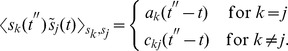 |
The pairwise spike-train correlation function is therefore given by
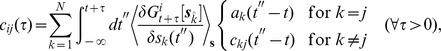 |
where we used the fact that  for any functional
  that does not
depend on
that does not
depend on  . The average of
the functional derivative has the intuitive meaning of a response kernel with
respect to a
. The average of
the functional derivative has the intuitive meaning of a response kernel with
respect to a  -shaped
perturbation of input
-shaped
perturbation of input  at time
 . Averaged over the
realizations of the stationary network activity this response can only depend on
the relative time
. Averaged over the
realizations of the stationary network activity this response can only depend on
the relative time  . In a homogeneous
random network, the input statistics (number of synaptic inputs and synaptic
weights) and the parameters of the internal dynamics are identical for each
cell, so that the temporal shape
. In a homogeneous
random network, the input statistics (number of synaptic inputs and synaptic
weights) and the parameters of the internal dynamics are identical for each
cell, so that the temporal shape  of the response kernel can be assumed to be the same for all neurons. The
synaptic coupling strength from neuron
of the response kernel can be assumed to be the same for all neurons. The
synaptic coupling strength from neuron  to neuron
  determines the
prefactor
determines the
prefactor  :
:
| (30) |
In this notation, the linear equation connecting the auto-correlations
 and the
cross-correlations
and the
cross-correlations  takes the form
| (31) |
Eq. (31) can be solved numerically or by means of Wiener-Hopf theory taking the
symmetry  into account [82].
Our aim is to find a simpler model which is equivalent to the LIF dynamics in the
sense that it fulfills the same equation (31). Let's  denote the vector of dynamic variables of this reduced
model. Analog to the original model, we define the cross-correlation for
denote the vector of dynamic variables of this reduced
model. Analog to the original model, we define the cross-correlation for
 and
and
 as
as
 |
(32) |
The simplest functional  consistent with
equation (31) is linear in
consistent with
equation (31) is linear in  .
Since we require equivalence only with respect to the ensemble averaged
quantities, i.e.
.
Since we require equivalence only with respect to the ensemble averaged
quantities, i.e.  , the reduced
activity and therefore
, the reduced
activity and therefore  can contain a
stochastic element which would disappear after averaging. The linear
functional
can contain a
stochastic element which would disappear after averaging. The linear
functional
| (33) |
with a pairwise uncorrelated, centralized white noise  (
( ) fulfills the
requirement, since for
) fulfills the
requirement, since for  and
and

 |
This equation has the same form as (31), so both models, within the linear
approximation, exhibit an identical relationship between the auto- and
cross-covariances. The physical meaning of the noise  is the variance caused by the spiking of the neurons.
The auto-correlation function of a spike train of rate
is the variance caused by the spiking of the neurons.
The auto-correlation function of a spike train of rate  has a
has a  -peak of weight
  .
The reduced model (33) exhibits such a
.
The reduced model (33) exhibits such a  -peak if we set
  .
A related approach has been pursued before (see Sec. 3.5 in [31]) to
determine the auto-correlation of the population averaged firing rate. This
similarity will be discussed in detail below.
.
A related approach has been pursued before (see Sec. 3.5 in [31]) to
determine the auto-correlation of the population averaged firing rate. This
similarity will be discussed in detail below.
So far, we considered a network without external drive, i.e. all spike trains
 originated from
within the network. If the network is driven by external input, each neuron
receives, in addition, synaptic input
originated from
within the network. If the network is driven by external input, each neuron
receives, in addition, synaptic input  from neurons outside the network. We assume uncorrelated external drive
 . In the reduced
model, this input constitutes a separate source of noise:
. In the reduced
model, this input constitutes a separate source of noise:
| (34) |
Here,  denotes the
convolution and
denotes the
convolution and  the response
kernel with respect to an external input. For simplicity, let's assume that
the shape of these kernels is identical for all pairs of pre- and postsynaptic
sources, i.e.
the response
kernel with respect to an external input. For simplicity, let's assume that
the shape of these kernels is identical for all pairs of pre- and postsynaptic
sources, i.e.  . If we further
absorb the synaptic amplitude of the external drive in the strength of the noise
. If we further
absorb the synaptic amplitude of the external drive in the strength of the noise
 , the linearized
dynamics (34) can be written in matrix notation
, the linearized
dynamics (34) can be written in matrix notation
| (35) |
with  . The reduced model
(35) can be solved directly by means of Fourier transform:
. The reduced model
(35) can be solved directly by means of Fourier transform:
| (36) |
The full covariance matrix follows by averaging over the sources of noise
 and
and
 as
as
 |
(37) |
The diagonal elements of  represent the
auto-covariances, the off-diagonal elements the cross-covariances. Both are
proportional to the driving noise
represent the
auto-covariances, the off-diagonal elements the cross-covariances. Both are
proportional to the driving noise  .
This is consistent with (31) which is a linear relationship between the cross-
and auto-covariances.
.
This is consistent with (31) which is a linear relationship between the cross-
and auto-covariances.
For networks which can be decomposed into homogeneous subpopulations, the
 dimensional system
(35) can be further simplified by population averaging. Consider, for example, a
homogeneous random network with purely inhibitory coupling. Assume that the
neurons are randomly connected with probability
dimensional system
(35) can be further simplified by population averaging. Consider, for example, a
homogeneous random network with purely inhibitory coupling. Assume that the
neurons are randomly connected with probability  and coupling strength
  . The average number of in/outputs per neuron
(in/out-degree) is thus given by
. The average number of in/outputs per neuron
(in/out-degree) is thus given by  .
By introducing the population averaged external input
.
By introducing the population averaged external input  , the averaged spiking noise
  , and the effective coupling strength
  , the dynamics of the population averaged activity
becomes
, the dynamics of the population averaged activity
becomes
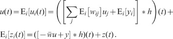 |
(38) |
Here we assumed that  is independent of
the presynaptic neuron
is independent of
the presynaptic neuron  and can be
replaced by
and can be
replaced by  . Note that this
replacement is exact for networks with homogeneous out-degree, i.e. if the
number of outgoing connections is identical for each neuron
. Note that this
replacement is exact for networks with homogeneous out-degree, i.e. if the
number of outgoing connections is identical for each neuron  . For large random networks with binomially distributed
out-degrees (e.g. Erdös-Rényi networks or random networks with
constant in-degree), (38) serves as an approximation.
. For large random networks with binomially distributed
out-degrees (e.g. Erdös-Rényi networks or random networks with
constant in-degree), (38) serves as an approximation.
To relate our approach to the treatment of finite-size fluctuations in [31], consider
the population-averaged dynamics (38) of a single population with mean firing
rate  . We set
 for all single
neuron noises
for all single
neuron noises  in order for the
reduced model's auto-covariances to reproduce the
in order for the
reduced model's auto-covariances to reproduce the  -peak of the spiking dynamics. In the population averaged
dynamics, this leads to the variance of the noise
-peak of the spiking dynamics. In the population averaged
dynamics, this leads to the variance of the noise  given by
 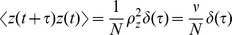 .
This agrees with the variance of the population rate in [31]. Therefore, the dynamics of
the population averaged quantity
.
This agrees with the variance of the population rate in [31]. Therefore, the dynamics of
the population averaged quantity  in (38) agrees with the earlier definition of a population averaged firing rate
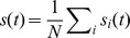 for the spiking
network [31].
for the spiking
network [31].
In equation (38), two distinct sources of noise appear: The noise due to external
uncorrelated activity  and the noise
 which is required
to obtain the
which is required
to obtain the  -peak of the
auto-correlation functions of the reduced model. The qualitative results of
“
Results
: Suppression of population-activity
fluctuations by negative feedback” and
“
Results
: Population-activity fluctuations in
excitatory-inhibitory networks”, however can be understood with
an even simpler model. As we are mainly concerned with the low-frequency
fluctuations, we only need a model with the same limit
-peak of the
auto-correlation functions of the reduced model. The qualitative results of
“
Results
: Suppression of population-activity
fluctuations by negative feedback” and
“
Results
: Population-activity fluctuations in
excitatory-inhibitory networks”, however can be understood with
an even simpler model. As we are mainly concerned with the low-frequency
fluctuations, we only need a model with the same limit  . As we normalized the kernel so that
  we can combine both sources of noise and require
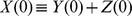 in (36) in the
zero frequency limit. Hence, in “
Results
: Suppression of
population-activity fluctuations by negative feedback” and
“
Results
: Population-activity fluctuations in
excitatory-inhibitory networks”, we consider the model
in (36) in the
zero frequency limit. Hence, in “
Results
: Suppression of
population-activity fluctuations by negative feedback” and
“
Results
: Population-activity fluctuations in
excitatory-inhibitory networks”, we consider the model
| (39) |
with a pairwise uncorrelated centralized white noise  to explain the suppression of fluctuations at low
frequencies.
to explain the suppression of fluctuations at low
frequencies.
As a second example, consider a random network composed of an excitatory and an
inhibitory subpopulation  and
and
 with population
sizes
with population
sizes  and
and
 , respectively.
Assume that each neuron receives excitatory and inhibitory inputs from
, respectively.
Assume that each neuron receives excitatory and inhibitory inputs from
 and
and
 with coupling
strengths
with coupling
strengths  and
and
 , respectively, and
probability
, respectively, and
probability  , such that the
average excitatory and inhibitory in/out-degrees are given by
, such that the
average excitatory and inhibitory in/out-degrees are given by  and
and  ,
respectively. The dynamics of the subpopulation averaged activities
,
respectively. The dynamics of the subpopulation averaged activities
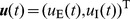 is given by (35)
with subpopulation averaged noise
is given by (35)
with subpopulation averaged noise 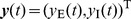 and
and 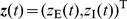 and effective
coupling
and effective
coupling
| (40) |
Here,  denotes the
effective coupling strength,
denotes the
effective coupling strength,  the effective balance parameter and
 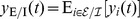 and
and 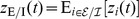 the
(sub)population averaged external and spiking sources of noise, respectively.
Again, the reduction of the
the
(sub)population averaged external and spiking sources of noise, respectively.
Again, the reduction of the  -dimensional linear dynamics to the two-dimensional dynamics
(40) is exact if the out-degrees are constant within each subpopulation. As
before, both sources of noise can be combined into a single source of noise, if
we are only interested in the low-frequency behavior of the model, leading to
the dynamics (39) with the effective coupling (40).
-dimensional linear dynamics to the two-dimensional dynamics
(40) is exact if the out-degrees are constant within each subpopulation. As
before, both sources of noise can be combined into a single source of noise, if
we are only interested in the low-frequency behavior of the model, leading to
the dynamics (39) with the effective coupling (40).
The linear theory is only valid in the domain of its stability, which is
determined by the eigenvalue spectrum of the effective coupling matrix
 . For random
coupling matrices, the eigenvalues are located within a circle with a radius
equal to the square root of the variance of the matrix entries [69]
. For random
coupling matrices, the eigenvalues are located within a circle with a radius
equal to the square root of the variance of the matrix entries [69]
 . Writing the
effective dynamics for the exponential kernel as a differential equation
. Writing the
effective dynamics for the exponential kernel as a differential equation
 , the eigenvalues
of the right hand side matrix
, the eigenvalues
of the right hand side matrix  are confined to a circle centered at
  in the complex plain with radius
  .
Given
.
Given  , eigenvalues might
exist which have a positive real part, leading to unstable dynamics. This
condition is indicated by the vertical dotted lines in Fig. 6 A–F and Fig. 7 B–D near
, eigenvalues might
exist which have a positive real part, leading to unstable dynamics. This
condition is indicated by the vertical dotted lines in Fig. 6 A–F and Fig. 7 B–D near  . Beyond this line, the linear model predicts an
explosive growth of fluctuations. In the LIF-network model, an unbounded growth
is avoided by the nonlinearities of the single-neuron dynamics.
. Beyond this line, the linear model predicts an
explosive growth of fluctuations. In the LIF-network model, an unbounded growth
is avoided by the nonlinearities of the single-neuron dynamics.
Response kernel of the LIF model
We now perform the formal linearization (30) for a network of  LIF neurons
  .
A similar approach has been employed in previous studies to understand the
population dynamics in these networks [12], [31]. We consider the input
.
A similar approach has been employed in previous studies to understand the
population dynamics in these networks [12], [31]. We consider the input
 received by neuron
 from the local
network, where
from the local
network, where  denotes the spike
train of the neuron
denotes the spike
train of the neuron  projecting to
neuron
projecting to
neuron  with synaptic
weight
with synaptic
weight  . Given the time
dependent firing rate
. Given the time
dependent firing rate  of each afferent,
and assuming small correlations and small synaptic weights, the total input to
neuron
of each afferent,
and assuming small correlations and small synaptic weights, the total input to
neuron  can be replaced by
a Gaussian white noise with mean
can be replaced by
a Gaussian white noise with mean  and variance
  ,
,
 |
(41) |
where  sums over all
synaptic inputs.
sums over all
synaptic inputs.  denotes the
amplitude of the postsynaptic potential evoked by synapse
denotes the
amplitude of the postsynaptic potential evoked by synapse  .
.  is the membrane
time constant of the model. In the stationary state, the firing rate of each
afferent is well described by the constant time average
is the membrane
time constant of the model. In the stationary state, the firing rate of each
afferent is well described by the constant time average  . The working point at which we perform the linearization
of the neural response (30) is then given by analog equations as (41), resulting
in a constant mean
. The working point at which we perform the linearization
of the neural response (30) is then given by analog equations as (41), resulting
in a constant mean  and variance
 . If the amplitude
of each postsynaptic potential is small compared to the distance of the membrane
potential to threshold, the dynamics of the LIF model can be approximated by a
diffusion process, employing Fokker-Planck theory [83]. The stationary firing rate
of the neuron is then given by [12], [31], [84]
. If the amplitude
of each postsynaptic potential is small compared to the distance of the membrane
potential to threshold, the dynamics of the LIF model can be approximated by a
diffusion process, employing Fokker-Planck theory [83]. The stationary firing rate
of the neuron is then given by [12], [31], [84]
 |
(42) |
with the reset voltage  , the threshold
voltage
, the threshold
voltage  and the refractory
time
and the refractory
time  . In homogeneous
random networks, the stationary rate (Fig. 7 A) is the same for all neurons. It is
determined in a self-consistent manner [12] as the fixed point of (42).
The stationary mean
. In homogeneous
random networks, the stationary rate (Fig. 7 A) is the same for all neurons. It is
determined in a self-consistent manner [12] as the fixed point of (42).
The stationary mean  and variance
 are determined by
the stationary rate. To determine the kernel (30) we need to consider how a
are determined by
the stationary rate. To determine the kernel (30) we need to consider how a
 -shaped deflection
in the input to this neuron at time point
-shaped deflection
in the input to this neuron at time point  affects its output up to linear order in the amplitude of the fluctuation. In
the stationary state, we may set
affects its output up to linear order in the amplitude of the fluctuation. In
the stationary state, we may set  .
It is therefore sufficient to focus on the effect of a single fluctuation
.
It is therefore sufficient to focus on the effect of a single fluctuation
| (43) |
We therefore ask how the density of spikes per time  of neuron
  ,
averaged over different realizations of the remaining inputs to neuron
,
averaged over different realizations of the remaining inputs to neuron
 , changes in
response to the fluctuation (43) of the presynaptic neuron
, changes in
response to the fluctuation (43) of the presynaptic neuron  in the limit of vanishing amplitude
  . This kernel
  (30) is identical to the impulse response of the neuron and can directly be
measured in simulation by trial averaging over many responses to the given
(30) is identical to the impulse response of the neuron and can directly be
measured in simulation by trial averaging over many responses to the given
 -deflection (43) in
the input (see Fig. 8 A).
For the theory of low-frequency fluctuations, we only need the integral of the
kernel, also known as the DC susceptibility,
-deflection (43) in
the input (see Fig. 8 A).
For the theory of low-frequency fluctuations, we only need the integral of the
kernel, also known as the DC susceptibility,
 |
(44) |
The second equality follows from the equivalence of the integral of the impulse
response and the step response in linear approximation [21], [33]. Following from
[41], both mean and variance are perturbed as  and
and  in response to a step
  in the afferent
rate
in the afferent
rate  . Moreover, we used
the chain rule
. Moreover, we used
the chain rule  . The variation of
the afferent firing rate hence co-modulates the mean and the variance and both
modulations need to be taken into account to derive the neural response [31]. Although
the finite amplitude of postsynaptic potentials has an effect on the response
properties [33], [34], the integral response is rather insensitive to the
granularity of the noise [33]. We therefore employ the diffusion approximation to
linearize the dynamics of the LIF neuron around its working point characterized
by the mean
. The variation of
the afferent firing rate hence co-modulates the mean and the variance and both
modulations need to be taken into account to derive the neural response [31]. Although
the finite amplitude of postsynaptic potentials has an effect on the response
properties [33], [34], the integral response is rather insensitive to the
granularity of the noise [33]. We therefore employ the diffusion approximation to
linearize the dynamics of the LIF neuron around its working point characterized
by the mean  and the variance
 of the total
synaptic input. In (44), we evaluate the partial derivatives of
of the total
synaptic input. In (44), we evaluate the partial derivatives of  with respect to
  and
and  using (42). First,
observe that by chain rule
using (42). First,
observe that by chain rule  .
We then again make use of the chain rule
.
We then again make use of the chain rule  .
Analog expressions hold for the derivative with respect to
.
Analog expressions hold for the derivative with respect to  . The first derivative yields
  , the one with respect to
  follows analogously, but with a negative sign. We
further observe that
follows analogously, but with a negative sign. We
further observe that  and
and
 with
with
 . Taken together,
we obtain the explicit result for (44)
. Taken together,
we obtain the explicit result for (44)
| (45) |
Note that the modulation of  results in a contribution to
  that is linear in
  , whereas the
modulation of
, whereas the
modulation of  causes a quadratic
dependence on
causes a quadratic
dependence on  . This expression
therefore presents an extension to the integral response presented in [21], [85]. Fig. 8 B shows the comparison
of the analytical expression (45) and direct simulation. The agreement is good
over a large range of synaptic amplitudes
. This expression
therefore presents an extension to the integral response presented in [21], [85]. Fig. 8 B shows the comparison
of the analytical expression (45) and direct simulation. The agreement is good
over a large range of synaptic amplitudes  in the case of constant background noise caused by small synaptic amplitudes
(here
in the case of constant background noise caused by small synaptic amplitudes
(here  for excitation and
 for inhibition).
For background noise caused by stronger impulses, the deviations are expected to
grow [33].
for inhibition).
For background noise caused by stronger impulses, the deviations are expected to
grow [33].
Population-activity spectra in the linear model: feedback vs. feedforward scenario
The recurrent linear neural dynamics defined in the previous section is
conveniently solved in the Fourier domain. The driving external Gaussian white
noise  is mapped to the
response
is mapped to the
response  by means of the
transfer matrix
by means of the
transfer matrix  . According to
(39), it is given by
. According to
(39), it is given by  . The covariance
matrix in the frequency domain, the spectral matrix, thus reads
. The covariance
matrix in the frequency domain, the spectral matrix, thus reads
| (46) |
where we used  and the
expectation operator
and the
expectation operator  represents an
average over noise realizations. To identify the effect of recurrence on the
network dynamics, we replace the local feedback input by a feedforward input
represents an
average over noise realizations. To identify the effect of recurrence on the
network dynamics, we replace the local feedback input by a feedforward input
 with spectral
matrix
with spectral
matrix  . The resulting
response firing rate is given by
. The resulting
response firing rate is given by  .
Assuming that the feedforward input
.
Assuming that the feedforward input  is uncorrelated to the external noise source
  (
( ) yields a
response spectrum
) yields a
response spectrum
| (47) |
Population-activity spectrum of the linear inhibitory network
In the Fourier domain, the solution of the mean-field dynamics (38) of the
inhibitory network is  . The
power-spectrum
. The
power-spectrum  hence becomes
| (48) |
using the spectrum of the noise  .
.
We compare this power-spectrum to the case where the feedback loop is opened,
i.e. where the recurrent input is replaced by feedforward input with unchanged
auto-statistics  , but which is
uncorrelated to the external input
, but which is
uncorrelated to the external input  .
The resulting power-spectrum is given by (47) as
.
The resulting power-spectrum is given by (47) as  .
.
Population-activity spectra of the linear excitatory-inhibitory network
In a homogeneous random network of excitatory and inhibitory neurons, the population averaged activity (40) can be solved in the Schur basis (9) introduced in “ Results : Population-activity fluctuations in excitatory-inhibitory networks”
 |
(49) |
with  and
and
 . The power of the
population rate therefore is
. The power of the
population rate therefore is
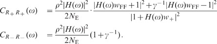 |
(50) |
The fluctuations of the excitatory and the inhibitory population follow as
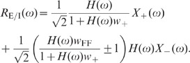 |
(51) |
So the power-spectra are
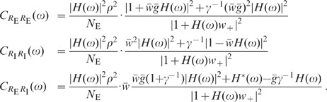 |
(52) |
Replacing the recurrent input of the sum activity  by activity
  with the same auto-statistics, but which is uncorrelated to the remaining input
into
with the same auto-statistics, but which is uncorrelated to the remaining input
into  (Fig. 5 D′) results in
the fluctuations
(Fig. 5 D′) results in
the fluctuations
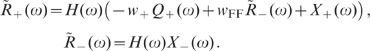 |
(53) |
The power-spectrum of the sum activity therefore becomes
 |
(54) |
If, alternatively, the excitatory and the inhibitory feedback terms
 and
and
 are replaced by
uncorrelated feedforward input
are replaced by
uncorrelated feedforward input  and
and  with
power-spectra
with
power-spectra  and
and
 (Fig. 5 C,D), the spectrum of
the sum activity reads
(Fig. 5 C,D), the spectrum of
the sum activity reads
 |
(55) |
The limit (14) for inhibition dominated networks with  can be obtained from this and the former expressions by
taking
can be obtained from this and the former expressions by
taking  and assuming
strong coupling
and assuming
strong coupling  .
.
Population averaged correlations in the linear EI network
In this subsection, we derive a self-consistency equation for the covariances in
a recurrent network. We start from (37) (we drop the superscript  of
of  for brevity) multiply by
  from left and its
transpose from right to obtain
from left and its
transpose from right to obtain
 |
(56) |
We assume a recurrent network of  excitatory and
  inhibitory
neurons, in which each neuron receives
inhibitory
neurons, in which each neuron receives  excitatory inputs of weight
  and
and  inhibitory inputs
of weight
inhibitory inputs
of weight  drawn randomly
from the presynaptic pool of neurons. To obtain a theory for the variances and
covariances at zero frequency (with
drawn randomly
from the presynaptic pool of neurons. To obtain a theory for the variances and
covariances at zero frequency (with  )
we may abbreviate
)
we may abbreviate  by
by
 . For a population
averaged theory, we need to replace in (56) the variances
. For a population
averaged theory, we need to replace in (56) the variances  of an individual neuron by the population average and
replace the covariance
of an individual neuron by the population average and
replace the covariance  for a given pair
of neurons
for a given pair
of neurons  by the average
over pairs that are statistically equivalent to
by the average
over pairs that are statistically equivalent to  . For a pair
  of neurons we will show that the set of equivalent pairs depends on the current
realization of the connectivity since unconnected pairs are not equivalent to
connected ones. Therefore it is necessary to first average the covariance matrix
over statistically equivalent neuron pairs given a fixed connectivity and to
subsequently average over all possible realizations of the connectivity. The
latter will be denoted as
of neurons we will show that the set of equivalent pairs depends on the current
realization of the connectivity since unconnected pairs are not equivalent to
connected ones. Therefore it is necessary to first average the covariance matrix
over statistically equivalent neuron pairs given a fixed connectivity and to
subsequently average over all possible realizations of the connectivity. The
latter will be denoted as  .
For compactness of the notation, first we perform the averaging for the general
case, where neuron
.
For compactness of the notation, first we perform the averaging for the general
case, where neuron  belongs to
population
belongs to
population  and neuron
 to population
 . We denote by
 ,
,  the sets of neuron indices belonging to populations
 and
and
 , respectively.
Subsequently replacing
, respectively.
Subsequently replacing  and
and
 by all possible
combinations
by all possible
combinations  , we obtain the
averaged self-consistency equations for the network. We denote the number of
incoming connections to a neuron of type
, we obtain the
averaged self-consistency equations for the network. We denote the number of
incoming connections to a neuron of type  from the population of neurons of type
  as
as  and the strength
of a synaptic coupling as
and the strength
of a synaptic coupling as  .
Rewriting the self-consistency equation (56) explicitly with indices yields
.
Rewriting the self-consistency equation (56) explicitly with indices yields
| (57) |
The last equation shows that for a connected pair  of neurons (
 or
or  ) either of the
first two sums contains a contribution
) either of the
first two sums contains a contribution  or
or  proportional to
the variance of the projecting neuron. We therefore need to perform the
averaging separately for connected and for unconnected pairs of neurons. We use
the notation
proportional to
the variance of the projecting neuron. We therefore need to perform the
averaging separately for connected and for unconnected pairs of neurons. We use
the notation
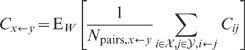 |
(58) |
for the average covariance over pairs of neurons of types  with a connection from neuron
  to neuron
  ,
where
,
where  is the number
neuron pairs connected in this way. An arrow to the right,
is the number
neuron pairs connected in this way. An arrow to the right,  , denotes a connection from neuron
  to neuron
  .
Note that we use the same letter
.
Note that we use the same letter  for the population averaged covariances and for the covariances of individual
pairs. The distinction can be made by the indices:
for the population averaged covariances and for the covariances of individual
pairs. The distinction can be made by the indices:  throughout indexes a single neuron,
  identifies one of the populations
  . We denote the covariance averaged over unconnected
pairs as
. We denote the covariance averaged over unconnected
pairs as
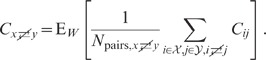 |
(59) |
We further use
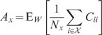 |
(60) |
for the integrated variance averaged over all neurons of type  . Connected and the unconnected averaged covariances
differ by the term proportional to the variance of the projecting neuron, as
mentioned above
. Connected and the unconnected averaged covariances
differ by the term proportional to the variance of the projecting neuron, as
mentioned above
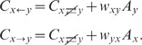 |
(61) |
As a consequence, we can express all quantities in terms of the averaged variance
(60) and the covariance averaged over unconnected pairs (59). We now proceed to
average the integrated variance over population  . Since there are no self-connections in the network, we
do not need to distinguish two cases here. Replacing
. Since there are no self-connections in the network, we
do not need to distinguish two cases here. Replacing  on the right hand side of (60), the first term of (57)
contributes
on the right hand side of (60), the first term of (57)
contributes
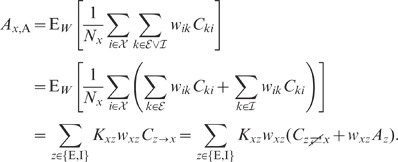 |
(62) |
From the second to the third step we used that the sum over  (
( ) yields non-zero
contributions only if neuron
) yields non-zero
contributions only if neuron  (
( ) connects to
neuron
) connects to
neuron  . This happens in
 (
( ) cases with the coupling weight
  (
( ). Therefore the
covariance averaged over connected pairs appears on the right hand side. In the
last line we used the relation (61) to express the connected covariance in terms
of the variance and the covariance over unconnected pairs. The second term in
(60) is identical because of the symmetry
). Therefore the
covariance averaged over connected pairs appears on the right hand side. In the
last line we used the relation (61) to express the connected covariance in terms
of the variance and the covariance over unconnected pairs. The second term in
(60) is identical because of the symmetry  . Up to here, the structure of the network only entered
in terms of the in-degree of the neurons. The contribution of the third term
follows from a similar calculation
. Up to here, the structure of the network only entered
in terms of the in-degree of the neurons. The contribution of the third term
follows from a similar calculation
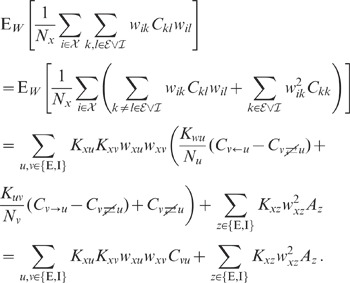 |
(63) |
From the second to the third step we assumed that among the  pairs of neurons
  projecting to neuron
  , the fraction
 has a connection
 . These pairs
contribute with the connected covariance. The connections in opposite direction
contribute the other term of similar structure. We ignore multiple and
reciprocal connections here, assuming the connection probability is low. We
introduce the shorthand
. These pairs
contribute with the connected covariance. The connections in opposite direction
contribute the other term of similar structure. We ignore multiple and
reciprocal connections here, assuming the connection probability is low. We
introduce the shorthand  for the
covariance averaged over all neuron pairs including connected and unconnected
pairs
for the
covariance averaged over all neuron pairs including connected and unconnected
pairs
| (64) |
This is the covariance which is observed on average when picking a pair of
neurons of type  and
and
 randomly. In this
step, beyond the in-degree, the structure of the network entered through the
expected number of connections between two populations. Taken all three terms
together, we arrive at
randomly. In this
step, beyond the in-degree, the structure of the network entered through the
expected number of connections between two populations. Taken all three terms
together, we arrive at
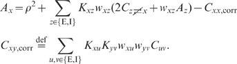 |
(65) |
The averaged covariances follow by similar calculations. Here we only need to
calculate the average over unconnected pairs  given by (59), because the connected covariance follows
from (61). The first sum in (57) contributes
given by (59), because the connected covariance follows
from (61). The first sum in (57) contributes
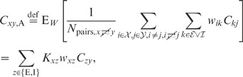 |
(66) |
where due to the absence of a direct connection between  and
and  ,
the term linear in the coupling and proportional to the variance is absent. From
the symmetry
,
the term linear in the coupling and proportional to the variance is absent. From
the symmetry  it follows that
the second term corresponds to an exchange of
it follows that
the second term corresponds to an exchange of  and
and  in the last expression. The third sum in (57) follows from an analog calculation
as before
in the last expression. The third sum in (57) follows from an analog calculation
as before
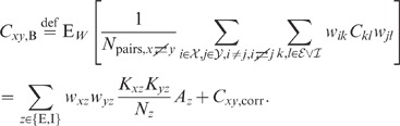 |
(67) |
In summary, the contributions from (66) and (67) together result in the self-consistency equation for the covariance
| (68) |
We now simplify the expressions by assuming that the in-degree of a neuron and
the incoming synaptic amplitudes do not depend on the type of the neuron, i.e.
that excitatory and inhibitory neurons receive statistically the same input.
Formally this means that we need to replace  by
by  ,
the number of incoming connections from population
,
the number of incoming connections from population  and
and  by
by  , the coupling
strength of a projection from a neuron of type
, the coupling
strength of a projection from a neuron of type  . The covariance
  then has two distinct contributions,
  that depends on the type of neurons
  ,
and
,
and  that does not. In
particular
that does not. In
particular  and
and
 do not depend on
 and we omit their
subscripts in the following. The variances fulfill
and we omit their
subscripts in the following. The variances fulfill
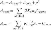 |
(69) |
the covariances satisfy
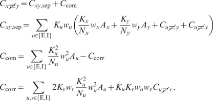 |
(70) |
The disjoint part  determines the
difference between the covariances for pairs of neurons of different type. Using
the parameters
determines the
difference between the covariances for pairs of neurons of different type. Using
the parameters  ,
,  ,
,  ,
,  , the explicit form is
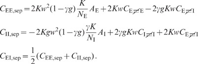 |
(71) |
Therefore, also the covariances in the network obey the relation
| (72) |
i.e. the mixed covariance can be eliminated and is given by the arithmetic mean
of the covariances between neurons of same type. In matrix representation with
the vector 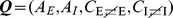 , the
self-consistency equation is
, the
self-consistency equation is
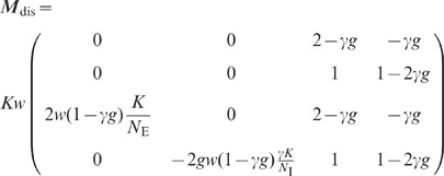 |
(73) |
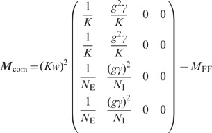 |
(74) |
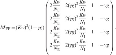 |
(75) |
The self consistent covariance can then be obtained by solving the system of linear equations
| (76) |
The numerical solution shows that the variances for excitatory and inhibitory
neurons are approximately the same, as depicted in Fig. 6 A. In the following we therefore
assume  and then solve
(76) for the covariances. With the abbreviation
and then solve
(76) for the covariances. With the abbreviation 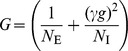 , the third and fourth line yields the equation for the
covariances
, the third and fourth line yields the equation for the
covariances
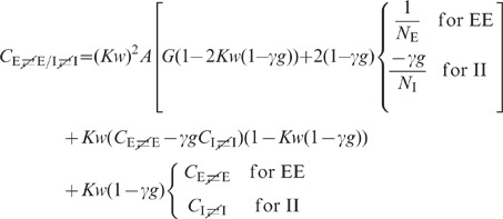 |
(77) |
The structure of the equation suggests to introduce the linear combination
 which
satisfies
which
satisfies
 |
(78) |
We solve (77) for  and
and
 and insert (78)
for
and insert (78)
for  to obtain the
covariances as
to obtain the
covariances as
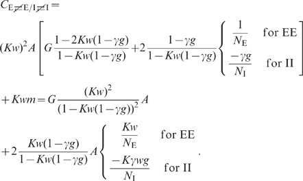 |
(79) |
The covariance  between
unconnected neurons can be related to the covariance between the incoming
currents this pair of neurons receives. Expressing the self-consistency (68) in
terms of the covariances averaged over connected and unconnected pairs (64)
uncovers the connection
between
unconnected neurons can be related to the covariance between the incoming
currents this pair of neurons receives. Expressing the self-consistency (68) in
terms of the covariances averaged over connected and unconnected pairs (64)
uncovers the connection
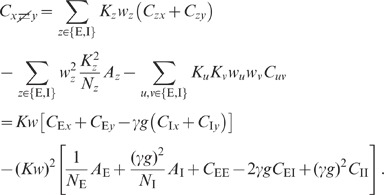 |
(80) |
This self-consistency equation yields the argument, why the shared-input
correlation  (19) cancels the
contribution
(19) cancels the
contribution  (20) due to
spike-train correlations in the covariance to the input currents (see Fig. 6 C,D). Rewriting (80) in
terms of these quantities results in
(20) due to
spike-train correlations in the covariance to the input currents (see Fig. 6 C,D). Rewriting (80) in
terms of these quantities results in
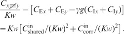 |
(81) |
If a self-consistent solution with small correlation  exists, the right hand side of (81) must be of the same
order of magnitude. The right hand side of this equation has a prefactor
exists, the right hand side of (81) must be of the same
order of magnitude. The right hand side of this equation has a prefactor
 which typically
is
which typically
is  (for the
parameters in Fig. 6,
(for the
parameters in Fig. 6,
 becomes larger
than
becomes larger
than  for
for
 ). The first term
in the bracket is proportional to the contribution of shared input, the second
term is due to correlations among pairs of different neurons. Each of these
terms is of order
). The first term
in the bracket is proportional to the contribution of shared input, the second
term is due to correlations among pairs of different neurons. Each of these
terms is of order  . Due to the
prefactor
. Due to the
prefactor  , however, the sum
of the two terms needs to be of order
, however, the sum
of the two terms needs to be of order  to fulfill the equation. Hence, the terms must have different signs to cause the
mutual cancellation.
to fulfill the equation. Hence, the terms must have different signs to cause the
mutual cancellation.
To illustrate how the correlation structure is affected by feedback, let us now consider the case where the feedback activity is perturbed (“feedforward scenario”). We start from (47) and, again, only consider the fluctuations at zero frequency,
| (82) |
First, we consider a manipulation that preserves the single-neuron statistics
 ,
,  and the pairwise correlations
  ,
,  within each
subpopulation, but neglects correlations
within each
subpopulation, but neglects correlations  between excitatory and inhibitory neurons. Formally, this corresponds to the
block diagonal correlation matrix
between excitatory and inhibitory neurons. Formally, this corresponds to the
block diagonal correlation matrix
| (83) |
Here, we have replaced the individual entries of the correlation matrix by the
corresponding subpopulation averaged correlations. The calculation of the
response auto- and cross-correlation  and
and  is similar as for
the expressions (63) and (67), with the difference that terms containing
is similar as for
the expressions (63) and (67), with the difference that terms containing
 are absent:
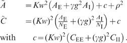 |
(84) |
As an alternative type of feedback manipulation, we assume that all correlations
are equal, irrespective of the neuron type. To this end, we replace all spike
correlations by the population average  .
Thus, the covariance matrix reads
.
Thus, the covariance matrix reads
| (85) |
The calculation follows the one leading to the expressions (63) and (67) and results in
 |
(86) |
Acknowledgments
We thank the three reviewers for their constructive comments.
Funding Statement
We acknowledge partial support by the Research Council of Norway (eVITA [eNEURO], Notur), the Helmholtz Alliance on Systems Biology, the Next-Generation Supercomputer Project of MEXT, Japan, EU Grant 15879 (FACETS), EU Grant 269921 (BrainScaleS), DIP F1.2, and BMBF Grant 01GQ0420 to BCCN Freiburg. The funders had no role in study design, data collection and analysis, decision to publish, or preparation of the manuscript.
References
- 1. Tripp B, Eliasmith C (2007) Neural populations can induce reliable postsynaptic currents without observable spike rate changes or precise spike timing. Cereb Cortex 17: 1830–1840. [DOI] [PubMed] [Google Scholar]
- 2. Zohary E, Shadlen MN, Newsome WT (1994) Correlated neuronal discharge rate and its implications for psychophysical performance. Nature 370: 140–143. [DOI] [PubMed] [Google Scholar]
- 3. Shadlen MN, Newsome WT (1998) The variable discharge of cortical neurons: Implications for connectivity, computation, and information coding. J Neurosci 18: 3870–3896. [DOI] [PMC free article] [PubMed] [Google Scholar]
- 4. Salinas E, Sejnowski TJ (2001) Correlated neuronal activity and the ow of neural information. Nat Rev Neurosci 2: 539–550. [DOI] [PMC free article] [PubMed] [Google Scholar]
- 5.von der Malsburg C (1981) The correlation theory of brain function. Internal report 81-2, Department of Neurobiology, Max-Planck-Institute for Biophysical Chemistry, Göttingen, Germany.
- 6. Bienenstock E (1995) A model of neocortex. Network: Comput Neural Sys 6: 179–224. [Google Scholar]
- 7.Abeles M (1991) Corticonics: Neural Circuits of the Cerebral Cortex. Cambridge: Cambridge University Press, 1st edition.
- 8. Diesmann M, Gewaltig MO, Aertsen A (1999) Stable propagation of synchronous spiking in cortical neural networks. Nature 402: 529–533. [DOI] [PubMed] [Google Scholar]
- 9. Tetzlaff T, Morrison A, Geisel T, Diesmann M (2004) Consequences of realistic network size on the stability of embedded synfire chains. Neurocomputing 58–60: 117–121. [Google Scholar]
- 10. Ecker AS, Berens P, Keliris GA, Bethge M, Logothetis NK (2010) Decorrelated neuronal firing in cortical microcircuits. Science 327: 584–587. [DOI] [PubMed] [Google Scholar]
- 11. van Vreeswijk C, Sompolinsky H (1996) Chaos in neuronal networks with balanced excitatory and inhibitory activity. Science 274: 1724–1726. [DOI] [PubMed] [Google Scholar]
- 12. Brunel N (2000) Dynamics of sparsely connected networks of excitatory and inhibitory spiking neurons. J Comput Neurosci 8: 183–208. [DOI] [PubMed] [Google Scholar]
- 13. Gerstner W (2000) Population dynamics of spiking neurons: fast transients, asynchronous states, and locking. Neural Comput 12: 43–89. [DOI] [PubMed] [Google Scholar]
- 14. Tetzlaff T, Rotter S, Stark E, Abeles M, Aertsen A, et al. (2008) Dependence of neuronal correlations on filter characteristics and marginal spike-train statistics. Neural Comput 20: 2133–2184. [DOI] [PubMed] [Google Scholar]
- 15. Kriener B, Tetzlaff T, Aertsen A, Diesmann M, Rotter S (2008) Correlations and population dynamics in cortical networks. Neural Comput 20: 2185–2226. [DOI] [PubMed] [Google Scholar]
- 16. Hertz J (2010) Cross-correlations in high-conductance states of a model cortical network. Neural Comput 22: 427–447. [DOI] [PubMed] [Google Scholar]
- 17. Renart A, De La Rocha J, Bartho P, Hollender L, Parga N, et al. (2010) The asynchronous state in cortical cicuits. Science 327: 587–590. [DOI] [PMC free article] [PubMed] [Google Scholar]
- 18. Stroeve S, Gielen S (2001) Correlation between uncoupled conductance-based integrate-and-fire neurons due to common and synchronous presynaptic firing. Neural Comput 13: 2005–2029. [DOI] [PubMed] [Google Scholar]
- 19. Tetzlaff T, Buschermöhle M, Geisel T, Diesmann M (2003) The spread of rate and correlation in stationary cortical networks. Neurocomputing 52–54: 949–954. [Google Scholar]
- 20. Moreno-Bote R, Parga N (2006) Auto- and crosscorrelograms for the spike response of leaky integrate-and-fire neurons with slow synapses. Phys Rev Lett 96: 028101. [DOI] [PubMed] [Google Scholar]
- 21. De la Rocha J, Doiron B, Shea-Brown E, Kresimir J, Reyes A (2007) Correlation between neural spike trains increases with firing rate. Nature 448: 802–807. [DOI] [PubMed] [Google Scholar]
- 22. Rosenbaum R, Josic K (2011) Mechanisms that modulate the transfer of spiking correlations. Neural Comput 23: 1261–1305. [DOI] [PubMed] [Google Scholar]
- 23. Battaglia D, Brunel N, Hansel D (2007) Temporal decorrelation of collective oscillations in neural networks with local inhibition and long-range excitation. Phys Rev Lett 99: 238106. [DOI] [PubMed] [Google Scholar]
- 24. Monteforte M, Wolf F (2010) Dynamical entropy production in spiking neuron networks in the balanced state. Phys Rev Lett 105 doi: 268104. [DOI] [PubMed] [Google Scholar]
- 25. Jahnke S, Memmesheimer RM, Timme M (2009) How chaotic is the balanced state? Front Comput Neurosci 3: 1–15. [DOI] [PMC free article] [PubMed] [Google Scholar]
- 26. Legenstein R, Maass W (2007) Edge of chaos and prediction of computational performance for neural circuit models. Neural Netw 20: 323–334. [DOI] [PubMed] [Google Scholar]
- 27. Jahnke S, Memmesheimer R, Timme M (2008) Stable irregular dynamics in complex neural networks. Phys Rev Lett 100: 048102. [DOI] [PubMed] [Google Scholar]
- 28. Toyoizumi T, Abbott LF (2010) Beyond the edge: Amplification and temporal integration by recurrent networks in the chaotic regime. Front Neurosci doi: 10.3389/conf.fnins.2010.03.00155. [DOI] [PMC free article] [PubMed] [Google Scholar]
- 29. Zillmer R, Livi R, Politi A, Torcini A (2006) Desynchronization in diluted neural networks. Phys Rev E 74: 036203. [DOI] [PubMed] [Google Scholar]
- 30. Ginzburg I, Sompolinsky H (1994) Theory of correlations in stochastic neural networks. Phys Rev E 50: 3171–3191. [DOI] [PubMed] [Google Scholar]
- 31. Brunel N, Hakim V (1999) Fast global oscillations in networks of integrate-and-_re neurons with low firing rates. Neural Comput 11: 1621–1671. [DOI] [PubMed] [Google Scholar]
- 32. Harris KD, Thiele A (2011) Cortical state and attention. Nat Rev Neurosci 12: 509–523. [DOI] [PMC free article] [PubMed] [Google Scholar]
- 33. Helias M, Deger M, Rotter S, Diesmann M (2010) Instantaneous non-linear processing by pulsecoupled threshold units. PLoS Comput Biol 6: e1000929. [DOI] [PMC free article] [PubMed] [Google Scholar]
- 34. Richardson MJE, Swarbrick R (2010) Firing-rate response of a neuron receiving excitatory and inhibitory synaptic shot noise. Phys Rev Lett 105: 178102. [DOI] [PubMed] [Google Scholar]
- 35. Fourcaud-Trocmé N, Hansel D, van Vreeswijk C (2003) Brunel (2003) How spike generation mechanisms determine the neuronal response to uctuating inputs. J Neurosci 23: 11628–11640. [DOI] [PMC free article] [PubMed] [Google Scholar]
- 36. Naundorf B, Geisel T, Wolf F (2005) Action potential onset dynamics and the response speed of neuronal populations. J Comput Neurosci 18: 297–309. [DOI] [PubMed] [Google Scholar]
- 37. Brunel N, Chance FS, Fourcaud N, Abbott LF (2001) Effects of synaptic noise and filtering on the frequency response of spiking neurons. Phys Rev Lett 86: 2186–2189. [DOI] [PubMed] [Google Scholar]
- 38. Nordlie E, Tetzlaff T, Einevoll GT (2010) Rate dynamics of leaky integrate-and-fire neurons with strong synapses. Front Comput Neurosci 4: 149. [DOI] [PMC free article] [PubMed] [Google Scholar]
- 39. Pressley J, Troyer TW (2009) Complementary responses to mean and variance modulations in the perfect integrate-and-fire model. Biol Cybern 101: 63–70. [DOI] [PubMed] [Google Scholar]
- 40. Knight BW (1972) The relationship between the firing rate of a single neuron and the level of activity in a population of neurons. J Gen Physiol 59: 767–778. [DOI] [PMC free article] [PubMed] [Google Scholar]
- 41. Köndgen H, Geisler C, Fusi S, Wang XJ, Lüscher HR, et al. (2008) The dynamical response properties of neocortical neurons to temporally modulated noisy inputs in vitro. Cereb Cortex 18: 2086–2097. [DOI] [PMC free article] [PubMed] [Google Scholar]
- 42. Boucsein C, Tetzlaff T, Meier R, Aertsen A, Naundorf B (2009) Dynamical response properties of neocortical neuron ensembles: multiplicative versus additive noise. J Neurosci 29: 1006–1010. [DOI] [PMC free article] [PubMed] [Google Scholar]
- 43. Blomquist P, Devor A, Indahl UG, Ulbert I, Einevoll GT, et al. (2009) Estimation of thalamocortical and intracortical network models from joint thalamic single-electrode and cortical laminarelectrode recordings in the rat barrel system. PLoS Comput Biol 5: e1000328. [DOI] [PMC free article] [PubMed] [Google Scholar]
- 44. Knight BW (1972) Dynamics of encoding in a population of neurons. J Gen Physiol 59: 734–766. [DOI] [PMC free article] [PubMed] [Google Scholar]
- 45. Lindner B, Schimansky-Geier L (2001) Transmission of noise coded versus additive signals through a neuronal ensemble. Phys Rev Lett 86: 2934–2937. [DOI] [PubMed] [Google Scholar]
- 46. Fourcaud N, Brunel N (2002) Dynamics of the firing probability of noisy integrate-and-fire neurons. Neural Comput 14: 2057–2110. [DOI] [PubMed] [Google Scholar]
- 47.Oppenheim A, Wilsky A (1996) Systems and signals. Upper Saddle River, NJ: Prentice Hall.
- 48. Troyer TW, Krukowski AE, Miller KD (2002) LGN input to simple cells and contrast-invariant orientation tuning: An analysis. J Neurophysiol 87: 2741–2752. [DOI] [PubMed] [Google Scholar]
- 49. Zhaoping L, Lewis A, Scarpetta S (2004) Mathematical analysis and simulations of the neural circuit for locomotion in lampreys. Phys Rev Lett 92: 198106. [DOI] [PubMed] [Google Scholar]
- 50. Murphy BK, Miller KD (2009) Balanced amplification: A new mechanism of selective amplification of neural activity patterns. Neuron 61: 635–648. [DOI] [PMC free article] [PubMed] [Google Scholar]
- 51. Moreno-Bote R, Renart A, Parga N (2008) Theory of input spike auto- and cross-correlations and their effect on the response of spiking neurons. Neural Comput 20: 1651–1705. [DOI] [PubMed] [Google Scholar]
- 52. Shadlen MN, Newsome WT (2001) Neural basis of a perceptual decision in the parietal cortex (area LIP) of the rhesus monkey. J Neurophysiol 86: 1916–1936. [DOI] [PubMed] [Google Scholar]
- 53. Gentet L, Avermann M, Matyas F, Staiger JF, Petersen CC (2010) Membrane potential dynamics of GABAergic neurons in the barrel cortex of behaving mice. Neuron 65: 422–435. [DOI] [PubMed] [Google Scholar]
- 54. Pernice V, Staude B, Cardanobile S, Rotter S (2011) How structure determines correlations in neuronal networks. PLoS Comput Biol 7: e1002059. [DOI] [PMC free article] [PubMed] [Google Scholar]
- 55. Pernice V, Staude B, Cardanobile S, Rotter S (2012) Recurrent interactions in spiking networks with arbitrary topology. Phys Rev E 85: 031916. [DOI] [PubMed] [Google Scholar]
- 56. Trousdale J, Hu Y, Shea-Brown E, Josic K (2012) Impact of network structure and cellular response on spike time correlations. PLoS Comput Biol 8: e1002408. [DOI] [PMC free article] [PubMed] [Google Scholar]
- 57. Softky WR, Koch C (1993) The highly irregular firing of cortical cells is inconsistent with temporal integration of random EPSPs. J Neurosci 13: 334–350. [DOI] [PMC free article] [PubMed] [Google Scholar]
- 58. Tetzlaff T, Geisel T, Diesmann M (2002) The ground state of cortical feed-forward networks. Neurocomputing 44–46: 673–678. [Google Scholar]
- 59. Mehring C, Hehl U, Kubo M, Diesmann M, Aertsen A (2003) Activity dynamics and propagation of synchronous spiking in locally connected random networks. Biol Cybern 88: 395–408. [DOI] [PubMed] [Google Scholar]
- 60. Aviel Y, Mehring C, Abeles M, Horn D (2003) On embedding synfire chains in a balanced network. Neural Comput 15: 1321–1340. [DOI] [PubMed] [Google Scholar]
- 61. Aviel Y, Horn D, Abeles M (2005) Memory capacity of balanced networks. Neural Comput 17: 691–713. [DOI] [PubMed] [Google Scholar]
- 62. Bi G, Poo M (1998) Synaptic modifications in cultured hippocampal neurons: Dependence on spike timing, synaptic strength, and postsynaptic cell type. J Neurosci 18: 10464–10472. [DOI] [PMC free article] [PubMed] [Google Scholar]
- 63. Gilson M, Burkitt AN, Grayden DB, Thomas DA, van Hemmen JL (2009) Emergence of network structure due to spike-timing-dependent plasticity in recurrent neuronal networks. I. Input selectivity - strengthening correlated input pathways. Biol Cybern 101: 81–102. [DOI] [PubMed] [Google Scholar]
- 64. Burkitt AN, Gilson M, van Hemmen J (2007) Spike-timing-dependent plasticity for neurons with recurrent connections. Biol Cybern 96: 533–546. [DOI] [PubMed] [Google Scholar]
- 65. Pfister JP, Tass PA (2010) Stdp in oscillatory recurrent networks: theoretical conditions for desynchronization and applications to deep brain stimulation. Front Comput Neurosci 454 doi: 10.3389/fncom.2010.00022. [DOI] [PMC free article] [PubMed] [Google Scholar]
- 66. Lindner B, Doiron B, Longtin A (2005) Theory of oscillatory firing induced by spatially correlated noise and delayed inhibitory feedback. Phys Rev E 72: 061919. [DOI] [PubMed] [Google Scholar]
- 67. Buice MA, Cowan JD, Chow CC (2009) Systematic uctuation expansion for neural network activity equations. Neural Comput 22: 377–426. [DOI] [PMC free article] [PubMed] [Google Scholar]
- 68. Sommers H, Crisanti A, Sompolinsky H, Stein Y (1988) Spectrum of large random asymmetric matrices. Phys Rev Lett 60: 1895–1898. [DOI] [PubMed] [Google Scholar]
- 69. Rajan K, Abbott L (2006) Eigenvalue spectra of random matrices for neural networks. Phys Rev Lett 97: 188104. [DOI] [PubMed] [Google Scholar]
- 70. Sompolinsky, Crisanti, Sommers (1988) Chaos in random neural networks. Phys Rev Lett 61: 259–262. [DOI] [PubMed] [Google Scholar]
- 71. Toyoizumi T, Rad KR, Paninski L (2009) Mean-field approximations for coupled populations of generalized linear model spiking neurons with markov refractoriness. Neural Comput 21: 1203–1243. [DOI] [PubMed] [Google Scholar]
- 72. Sirovich L, Omurtag A, Knight BW (2000) Dynamics of neuronal populations: The equilibrium solution. SIAM J Appl Math 60: 2009–2028. [Google Scholar]
- 73. Jacobsen M, Jensen AT (2007) Exit times for a class of piecewise exponential markov processes with two-sided jumps. Stoch Proc Appl 117: 1330–1356. [Google Scholar]
- 74.Cox DR (1962) Renewal Theory. Science Paperbacks. London: Chapman and Hall.
- 75. Nawrot MP, Boucsein C, Rodriguez Molina V, Riehle A, Aertsen A, et al. (2008) Measurement of variability dynamics in cortical spike trains. J Neurosci Methods 169: 374–390. [DOI] [PubMed] [Google Scholar]
- 76. Chizhov AV, Graham LJ (2008) Efficient evaluation of neuron populations receiving colored-noise current based on a refractory density method. Phys Rev E 77: 011910. [DOI] [PubMed] [Google Scholar]
- 77. Meyer C, van Vreeswijk C (2002) Temporal correlations in stochastic networks of spiking neurons. Neural Comput 14: 369–404. [DOI] [PubMed] [Google Scholar]
- 78.Hebb DO (1949) The organization of behavior: A neuropsychological theory. New York: John Wiley & Sons.
- 79. Helias M, Rotter S, Gewaltig M, Diesmann M (2008) Structural plasticity controlled by calcium based correlation detection. Front Comput Neurosci 2 doi:10.3389/neuro.10.007.2008. [DOI] [PMC free article] [PubMed] [Google Scholar]
- 80. Loebel A, Silberberg G, Helbig D, Markram H, Tsodyks M, et al. (2009) Multiquantal release underlies the distribution of synaptic efficacies in the neocortex. Front Comput Neurosci 3: 27. [DOI] [PMC free article] [PubMed] [Google Scholar]
- 81. Gewaltig MO, Diesmann M (2007) NEST (NEural Simulation Tool). Scholarpedia 2: 1430. [Google Scholar]
- 82. Hawkes A (1971) Point spectra of some mutually exciting point process. J R Statist Soc Ser B 33: 438–443. [Google Scholar]
- 83.Risken H (1996) The Fokker-Planck Equation. Berlin: Springer Verlag.
- 84. Siegert AJ (1951) On the first passage time probability problem. Phys Rev 81: 617–623. [Google Scholar]
- 85. Helias M, Deger M, Diesmann M, Rotter S (2010) Equilibrium and response properties of the integrate-and-fire neuron in discrete time. Front Comput Neurosci 3 doi:10.3389/neuro.10.029.2009. [DOI] [PMC free article] [PubMed] [Google Scholar]
- 86.Tuckwell HC (1988) Introduction to Theoretical Neurobiology, volume 1. Cambridge: Cambridge University Press.
- 87. Rotter S, Diesmann M (1999) Exact digital simulation of time-invariant linear systems with applications to neuronal modeling. Biol Cybern 81: 381–402. [DOI] [PubMed] [Google Scholar]