MetaVelvet: an extension of Velvet assembler to de novo metagenome assembly from short sequence reads

Abstract

An important step in ‘metagenomics’ analysis is the assembly of multiple genomes from mixed sequence reads of multiple species in a microbial community. Most conventional pipelines use a single-genome assembler with carefully optimized parameters. A limitation of a single-genome assembler for de novo metagenome assembly is that sequences of highly abundant species are likely misidentified as repeats in a single genome, resulting in a number of small fragmented scaffolds. We extended a single-genome assembler for short reads, known as ‘Velvet’, to metagenome assembly, which we called ‘MetaVelvet’, for mixed short reads of multiple species. Our fundamental concept was to first decompose a de Bruijn graph constructed from mixed short reads into individual sub-graphs, and second, to build scaffolds based on each decomposed de Bruijn sub-graph as an isolate species genome. We made use of two features, the coverage (abundance) difference and graph connectivity, for the decomposition of the de Bruijn graph. For simulated datasets, MetaVelvet succeeded in generating significantly higher N50 scores than any single-genome assemblers. MetaVelvet also reconstructed relatively low-coverage genome sequences as scaffolds. On real datasets of human gut microbial read data, MetaVelvet produced longer scaffolds and increased the number of predicted genes.

INTRODUCTION

The pioneering work in metagenomics analysis was done by Venter et al. (1) for the Sargasso Sea environmental genome analysis. The bulk extraction of diverse microbial genomes from the environment without prior laboratory cultivation is one of the most fascinating features of metagenomics. There have been several analyses of various kinds of environmental genomes, such as (2). Recent progress in next-generation sequencing technology offers more opportunities for metagenome analyses and permits deep sequencing (especially the Illumina Genome Analyzer) for highly diverse microbial populations. However, while a number of metagenomes have been sequenced using next-generation sequencers and deposited into public genome databases, only a few studies have reported their assembly results (3,4). This is mainly because of the short length of sequence reads from next-generation sequencers. Furthermore, there is also a fundamental difficulty of metagenomics analysis compared with isolated genome analysis. In a microbial community, the number of strains is initially unknown, and their relative abundance is also unknown and potentially skewed (5).

There are currently a few ‘de novo’ assemblers specifically devoted to metagenome assembly from mixed sequence reads of multiple species (6,7). In contrast, there are two alternative approaches to ‘de novo’ analysis for mixtures of sequence reads from environmental genomes: (i) applying a single-genome assembler to metagenome sequence reads (3,4,8,9) and (ii) binning (clustering) a set of sequence reads into different clusters (10,11,12). However, single-genome assemblers were not designed to assemble multiple genomes from a mixture of sequence reads with nonuniform sequence coverages. On the other hand, the unsupervised binning of sequence reads also has the limitation of clustering the input reads based only on k-mer frequencies in the ‘short’ reads without assembly. A third approach (not de novo) is comparative genome analysis mapping reads or aligning contigs to reference genomes (5,13,14). Unfortunately, the comparative approach cannot cover any microbial species whose reference genomes or closely related genomes have not been assembled.

In spite of such difficulties, our primary goal was ‘to reconstruct the whole genomes of multiple species in a microbial community, particularly from very short sequence reads generated by a next-generation sequencer’. To accomplish such de novo metagenome assembly, we extended a single-genome assembly program (assembler), named ‘Velvet’, using a de Bruijn graph (15,16), to a metagenome assembly program for mixed short reads of multiple species. A de Bruijn graph is a data structure for genome assembly programs that compactly represents an overlap between short reads. The de Bruijn graph-based assembly program identifies the overlaps between reads using a de Bruijn graph and merges the reads to reconstruct longer sequences. Note that the de Bruijn graph representation was first used for sequencing by hybridization by (17).

Our fundamental strategy for metagenome assembly was to consider that a de Bruijn graph constructed from mixed sequence reads of multiple species is equivalent to the mixture of multiple de Bruijn subgraphs, each of which is constructed from sequence reads of individual species and to decompose the mixed de Bruijn graph into individual subgraphs and build scaffolds based on each decomposed subgraph (Figure 1).

Figure 1.

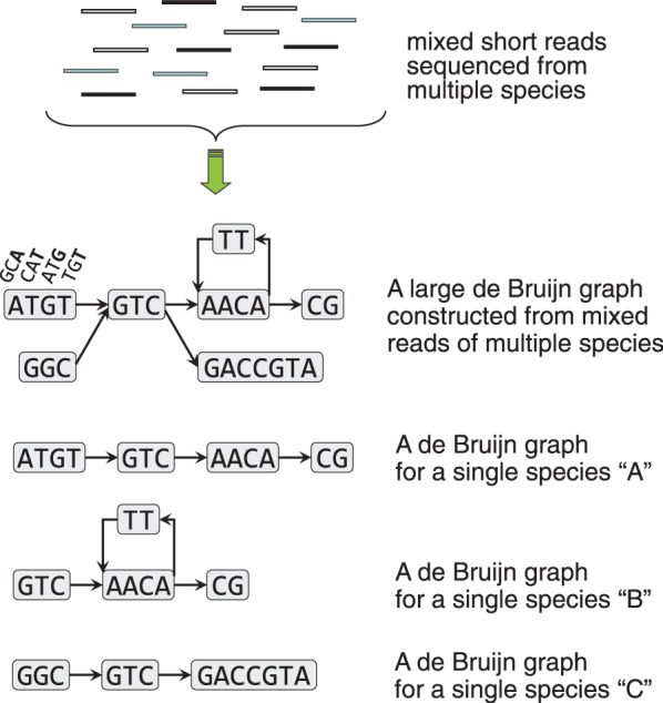
The MetaVelvet strategy to decompose a mixed de Bruijn graph.

From the ‘monotonic increasing’ property of de Bruijn graph construction, it is obvious that the de Bruijn graph, denoted dBg(X₁ + X₂ + ··· X_m), constructed from the mixture, denoted X₁ + X₂ + ··· X_m, of sequence reads of multiple species contains each de Bruijn graph dBg(X_i) constructed from sequence reads X_i of individual species (1 ≤ i ≤ m) as subgraphs. Therefore, it clearly holds that

and the strategy of decomposing the de Bruijn graph is proven to be reasonable.

In the decomposition step of the de Bruijn graph of multiple species, the coverage (abundance) difference and graph connectivity are used to distinguish a subgraph composed of a single species from the other subgraphs, where the ‘coverage’ is defined to be k-mer frequency in the input sequence reads. When two subgraphs, say dBg(X₁) and dBg(X₂), contained in the main de Bruijn graph have distinguishable read coverages, we disconnect the two subgraphs based on the coverage difference, such that metagenome assembly problem would be reduced to a set of easier problems of single-genome assemblies based on the decomposed subgraphs dBg(X₁) and dBg(X₂). For the graph disconnection task, an algorithm to identify shared nodes was developed, called the ‘chimeric node’, between two subgraphs dBg(X₁) and dBg(X₂). On the other hand, when two species are sufficiently evolutionarily distant, two genomes cannot share any k-mers, and therefore the main de Bruijn graph constructed from mixed reads of two species must be already separated and consist of two separated subgraphs.

For simulated datasets, the MetaVelvet metagenome assembler succeeded in generating higher N50 scores than any comparable assemblers and produced high-quality scaffolds, as well as separate genome assemblies from isolated species sequence reads, where the N50 score is a standard statistical measure that evaluates the assembly quality and indicates the scaffold length such that 50% of the assembled sequences lie in scaffolds of this size or larger. The scaffolds with longer N50 scores especially benefit the identification of protein-coding genes. In fact, the number of predicted complete protein-coding genes from MetaVelvet scaffolds is significantly larger than that produced by any of the other assemblers. Furthermore, MetaVelvet could reconstruct relatively low-coverage genome sequences as scaffolds. On real datasets of human gut microbial short read data sequenced as part of the MetaHIT project (3), our MetaVelvet produced longer scaffolds, and significantly increased the number of predicted genes. The source code of MetaVelvet is freely available at http://metavelvet.dna.bio.keio.ac.jp under the GNU General Public License and is distributed as a bundle with ‘Velvet’.

MATERIALS AND METHODS

Information obtained from the DNA sequencer is a set of sequence fragments, called reads, rather than the entire genomic DNA sequence. Therefore, genome assembly is required to reconstruct the original genome sequence from sequence reads. Although each read is short, it is possible to reconstruct longer sequences, called contigs, by identifying an overlap between reads and merging the reads. Genome assembly is generally performed in the following steps:

1. The input is a set of the nucleotide sequences of DNA fragments.

2. The overlap between every pair of sequences is calculated by pairwise alignment.

3. A pair of sequences with significant overlap is merged to obtain a longer sequence.

4. The above Steps 2 and 3 are repeated.

If a large amount of reads sufficient to ‘cover’ the genome are given to the assembly program, overlaps exist between the reads and the contigs are obtained by merging the reads. The term ‘coverage’ for a position in a contig is defined as the number of reads that overlap at that position. The ‘coverage’ of a ‘contig’ is defined to be the average of coverages for all positions in the contig.

First, we briefly review the de Bruijn graph-based assembly method for single genomes and the Velvet assembler upon which our method is based. Second, we describe our extension of Velvet to metagenome assembly.

De Bruijn graph-based assembly

The previous conventional assembly method is based on the so-called ‘overlap graph’, where each read is assigned to a node and an edge connects two nodes if the corresponding reads overlap. The assembly problem is reduced to finding a path visiting every node exactly once in the overlap graph, that is, a Hamiltonian path problem. However, the Hamiltonian path problem is nondeterministic polynomial time-complete (NP-complete). Furthermore, the overlap-graph-based assembly method cannot work effectively when applied to very short reads generated from a next-generation sequencer, because there are so many short overlaps between short reads and most of these overlaps are false. Therefore, several de novo assembly methods based on de Bruijn graphs have been proposed for short reads generated from next-generation sequencers (15,18,19,20). A de Bruijn graph is a data structure that compactly represents an overlap between short reads. A notable difference between a de Bruijn graph and an overlap graph is that each k-mer (word of length k) instead of a read is assigned to a node, and thus, the size of a de Bruijn graph becomes independent of the size of the input of reads. The detailed definition of de Bruijn graph is shown below.

Given a set of sequence reads, the de Bruijn graph-based assemblers first break each read according to a predefined k-mer length. It is clear that two adjacent k-mers in the read overlap at k − 1 nucleotides. Second, a directed graph (de Bruijn graph) is constructed from the given sequence reads as follows: each overlapping (k − 1)-mer is encoded into a node in the directed graph so that each k-mer is represented by a directed edge in the graph. Each k-mer is encoded into a directed edge that connects a node labeled the first (k − 1)-mer of the k-mer and a node labeled the second (k − 1)-mer. On the constructed de Bruijn graph, each read is mapped to a path traversing the graph. Therefore, the assembly (reconstruction) of the target genome from the de Bruijn graph can be reduced to finding a Eulerian path (Figure 2).

Figure 2.

Illustration of de Bruijn graph-based assembly.

Brief outline of Velvet and its de Bruijn graph representation

In Velvet, the de Bruijn graph is implemented slightly differently, such that each node represents a series of overlapping k-mers where adjacent k-mers overlap by k − 1 nucleotides. Each node is labeled by the sequence of the last nucleotides of the k-mers (Figure 1). Furthermore, each node is attached to a twin node that represents the reverse series of reverse complement k-mers for reads from opposite strands.

For each input read, the ordered set of overlapping k-mers is defined. Next, the ordered set is cut whenever an overlap with another read begins or ends. For each uninterrupted ordered subset of original k-mers, a node is created. Two nodes can be connected by a directed edge. If two nodes are connected, the last k-mer of an origin node overlaps by k − 1 nucleotides with the first of its destination node. New directed edges are created by tracing the read through the constructed graph.

Second, Velvet executes three functions, ‘simplification’ for node merging, and ‘removing tips’ and ‘removing bubbles’ for error removal. Simplification merges two nodes where one node has only one outgoing edge and the other has only one incoming edge. A ‘tip’, which is defined as a chain of nodes disconnected on one end, is removed. A ‘bubble’, which is defined as two redundant paths that start and end at the same nodes and contain similar sequences, is merged. Those tips and bubbles are created by sequencing errors or biological variants, such as single nuleotide polymorphisms (SNPs). Then, the ‘coverage of a node’ is defined as the coverage of the contig assigned to the node.

Finally, two functions, ‘Pebble’ and ‘Rock Band’, are called for constructing the scaffold and for repeat resolution using paired-end information and long read information. In these functions, Velvet distinguishes the unique nodes from the repeat nodes based on node coverage. A repeat node represents a sequence that occurs several times in the genome. Simply put, a repeat node is at a crossing point between two paths with multiple incoming and outgoing edges. Note that in multiple genome assembly, the nodes at a crossing point between two paths are not necessarily repeats. Such nodes are sometimes shared between the genomes of two closely related species and represent orthologous sequences, conserved sequences (such as rRNA sequences) and horizontal transfer sequences.

Extension to metagenome assembly

The MetaVelvet assembler consists of four major steps: [1] Construction of a de Bruijn graph from the input reads. [2] Detection of multiple peaks on k-mer frequency distribution. [3] Decomposition of the constructed de Bruijn graph into individual subgraphs. [4] Assembly of contigs and scaffolds based on the decomposed subgraphs. The flowchart of MetaVelvet is shown in Figure 3.

Figure 3.

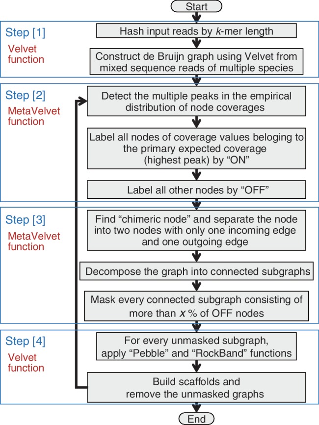
Flowchart of the main procedure of MetaVelvet.

In Step [1], for a given set of mixed sequence reads generated from multiple species, MetaVelvet constructs the main de Bruijn graph using Velvet functions. In Step [2], MetaVelvet calculates the histogram of k-mer frequencies and detects multiple peaks on the histogram, each of which would correspond to the genome of one species in a microbial community. The expected frequencies of k-mer occurrences were shown to follow a Poisson distribution in a single-genome assembly (21) and the expected k-mer frequencies in metagenome assembly were shown to follow a mixture of Poisson distributions (12). Hence, MetaVelvet approximates the empirical histogram of k-mer frequencies by a mixture of Poisson distributions and detects multiple peaks in the Poisson mixture. Furthermore, MetaVelvet classifies every node into one peak of the Poisson mixture. In Step [3], MetaVelvet distinguishes a subgraph composed of nodes belonging to a same peak from the other subgraphs in the main de Bruijn graph. MetaVelvet identifies shared nodes (chimeric nodes) between two subgraphs and disconnects two subgraphs by separating the shared nodes. In step [4], MetaVelvet builds contigs and scaffolds based on the decomposed subgraphs using Velvet functions.

The essential part of Step [3] is to design and develop an algorithm to identify and separate ‘chimeric nodes’ in the main de Bruijn graph. If two species contain a common or similar subsequence in their genomes, the main de Bruijn graph contains a node assigned to the subsequence with two incoming edges and two outgoing edges, one of which comes from one species and the other comes from the other species. On the other hand, if the genome of one species contains a repeat subsequence (that is, a subsequence with multiple occurrences in the genome), the de Bruijn graph also contains a node assigned to the repeat subsequence with two incoming edges and two outgoing edges. All other nodes in the main de Bruijn graph must have only one incoming edge and one outgoing edge. To distinguish the chimeric node from the repeat node, the method uses coverage difference. Although the origin nodes of two incoming edges for the repeat node have the same k-mer frequencies, the origin nodes of two incoming edges for the chimeric node belong to two different species and hence have different k-mer frequencies. The formal definition of ‘chimeric node’ is given as a crossing node satisfying the following three conditions: (i) (necessary condition) the number of incoming edges is 2 and the number of outgoing edges is 2; (ii) (sufficient condition) the origin nodes of two incoming edges (a and b) belong to two different peaks and the destination nodes of outgoing edges (c and d) also belong to the same two peaks as the origin nodes and (iii) (sufficient condition) the chimeric node has a confluent node coverage of the two origin nodes. More precisely, the node coverage of the candidate chimeric node should be between (a.cov + b.cov + c.cov + d.cov)/2 × (1 − y) and (a.cov + b.cov + c.cov + d.cov)/2 × (1 + y), where a.cov represents the node coverage of a node a and y is a parameter in MetaVelvet called ‘allowable coverage difference’. An example of the determination of a chimeric node is given in Figure 4.

Figure 4.

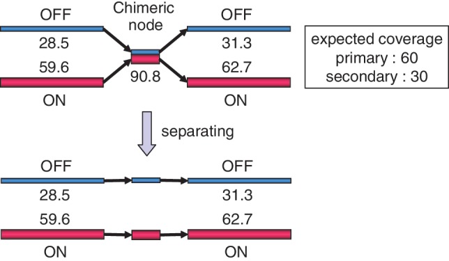
An example of a chimeric node and its resolution by separating the node. The node is chimeric because [(28.5 + 59.6) + (31.3 + 62.7)]/2 ≃ 90.8.

Once a candidate for chimeric node is identified, the candidate node is checked for ‘consistency’ with paired-end information. If a significant amount of paired-end reads connect an origin node of an incoming edge of the chimeric node with a destination node labeled differently from the origin node (that is, the paired-end reads connect an origin node labeled ON and a destination node labeled OFF or vice versa, as shown in Figure 4), the candidate node is discarded.

The detailed procedure of MetaVelvet is as follows:

• [1]
  Construction of the de Bruijn graph:

  • 1.
    For a given set of sequence reads generated from mixed species, construct a de Bruijn graph by calling Velvet first stage functions.
• [2]
  Detection of multiple peaks on k-mer frequencies:

  • 2.
    Calculate the empirical distribution of ‘length-weighted frequencies’ of node coverages, where a node coverage is assigned to each node by Velvet on the construction of the de Bruijn graph (Figure 5).
  • 3.
    Approximate the empirical distribution by a mixture of Poisson distributions and detect multiple peaks in the Poisson mixture. Then, the highest peak of expected coverage is chosen as the ‘primary expected coverage’, and the next highest is chosen as the ‘secondary expected coverage’.
  • 4.
    Classify every node into one distribution of the Poisson mixture by calculating its posterior probability for the node coverage value.
• [3]
  Decomposition of the de Bruijn graph:

  • 5.
    (Decomposition by connectivity) Decompose the initial de Bruijn graph into connected subgraphs.
  • 6.
    (Decomposition by coverage value) If the coverage of a node belongs to the primary expected coverage, the node is classified as a ‘primary node’. Subsequently, the primary nodes are labeled as ‘ON’ and the other nodes are labeled as ‘OFF’. Then, a chimeric node is detected as having two incoming edges whose origin nodes are labeled ON and OFF, and two outgoing edges whose destination nodes are labeled ON and OFF, and having a coverage value mostly equal (within 5% difference by default) to the average between the sum of the coverage values of the two origin nodes and the sum of the two destination nodes. Second, check the consistency of the ON and OFF labeling for the two origin nodes and two destination nodes using paired-end information. If the consistency is satisfied, resolve every chimeric node by separating the node into two nodes with only one incoming edge and one outgoing edge, whose origin and destination nodes have the same label, as shown in Figure 4. After separating the chimeric nodes, further decompose the resulting graph into connected subgraphs.
  • 7.
    If a connected subgraph consists of more than x% (a predefined parameter, the default is set to 100%) of nodes labeled ‘ON’, the subgraph is unmasked. All other subgraphs are masked.
• [4]
  Assembly of contigs and scaffolds:

  • 8.
    Apply the Velvet functions to the unmasked subgraphs to build contigs and then apply Pebble and Rock Band functions to build scaffolds.
  • 9.
    Remove the unmasked subgraphs and recursively apply Step 2–8 to the remaining de Bruijn graph until no node remains.

It might be thought that in Substep 3 above, a chimeric node could have the highest expected coverage. However, the contigs of chimeric nodes are very short compared with the unique nodes; therefore, the length-weighted frequencies of coverage values for the chimeric nodes do not form any significant peaks.

Figure 5.

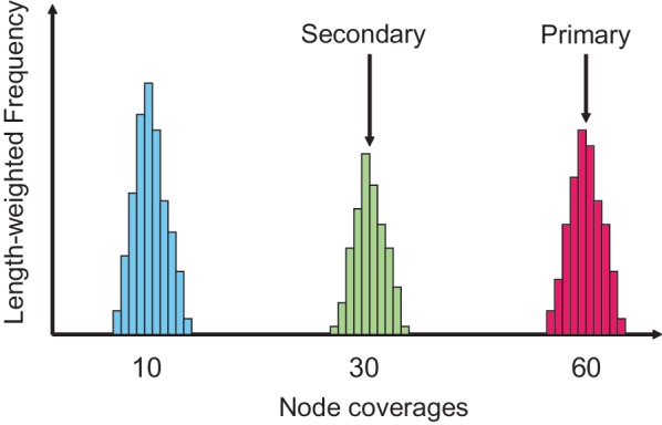
Detection of multiple peaks in the histogram of coverage values of the nodes.

EXPERIMENTAL RESULTS

The performance of the MetaVelvet assembler was tested on simulated datasets and on real metagenome datasets obtained from human gut microbiome. The method was compared with the naive use of two single-genome assemblers, Velvet (15) and SOAPdenovo (22), and the recently proposed metagenome assembler Meta-IDBA (6). Furthermore, for the simulated datasets, we compared our results with those of a single-genome assembly from pure sequence reads of each single-isolate genome. We compared the following standard statistical measures to evaluate the performance of the assemblers for short read assembly and metagenome assembly: the number of scaffolds, the total length of scaffolds and N50, where N50 indicates the scaffold length such that 50% of the de novo assembled sequences lie in scaffolds of this size or larger. The precise definition of N50 is as follows. Let |A| denote the length of a sequence (contig, scaffold or genome) A. Let S₁, S₂, … , S_n denote the list of scaffolds in descending order of length as output by an assembler. Let L denote the total length of all scaffolds, that is, . Then, N50 is defined by the following equation:

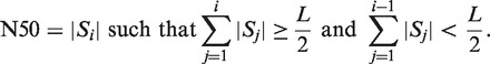(1)

Furthermore, from the assembled scaffolds, protein-coding genes (that is, open reading frames (ORFs)) were predicted using the MetaGene (23) software, and the number of predicted genes was compared.

For the simulated datasets, the following genome cover rate was calculated per species: the ‘cover rate’ of genome A is defined by the ratio of the sum of all scaffold lengths that are best aligned to genome A divided by the length of genome A. More precisely, the cover rate is defined by the following equation:

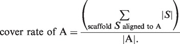Furthermore, we counted the total length of chimeric scaffolds. We determined whether a scaffold was chimeric by the following procedure. First, we calculated the best hit alignments between a scaffold and the set of input reference genomes using BLAST. Second, if a scaffold has more than two subsequences that are aligned to different genomes, and those subsequences are longer than 1% of the scaffold length, the scaffold was determined as chimeric.

Performances on simulated datasets

We used the ‘DWGSIM package’ in the DNAA package (available at http://sourceforge.net/projects/dnaa/) to artificially generate metagenome sequence reads. The read length was set at 80 bp, ‘very short’. The average and standard deviation of insert size for paired-end reads were set at 500 and 50 bp, respectively. Sequencing error rate was set at 1%. For species abundance settings, we applied the ‘log-normal distribution’, because the log-normal distribution has been generally used to model microbial abundance distributions (24). Thus, the simulated metagenomic datasets were generated to yield a k-mer coverage histogram following log-normal distribution.

To test the performances on various taxonomic levels of diversity, we constructed four datasets with different taxonomic levels of diversity, that is, ‘order level’, ‘family level’, ‘genus level’, and ‘species level’. In general, at lower taxonomic levels, the genomes of two different species become more similar and share more k-mer subsequences. Therefore, the separation of the input sequence reads and the decomposition of the de Bruijn graph become harder and the metagenome assembly problem from mixed sequence reads of multiple species becomes harder at lower taxonomic levels. We selected the four datasets to range from distant taxonomic level (that is, order level) to closer taxonomic level (species level). For each dataset, 20 species genomes were selected, and short read datasets were generated from the 20 genomes. (The lists of the 20 selected genomes for each taxonomic level are provided in Supplementary Tables S1–S4.)

Artificially generated short reads were assembled by two short read single-genome assemblers, Velvet (15) and SOAPdenovo (22), and two metagenome assemblers, Meta-IDBA (6), MetaVelvet, with default parameters except for SOAPdenovo, which used the ‘-M 3’ option, a parameter considered suitable for metagenomics assembly (3). The versions of these software packages used were Velvet 1.1.06, SOAPdenovo 1.05, Meta-IDBA 0.19 and MetaVelvet 1.3.1. Since Meta-IDBA does not have the scaffolding function, contigs instead of scaffolds were used to evaluate Meta-IDBA.

Order-level metagenomic dataset

Six orders from the ‘Alphaproteobacteria’ class and 14 orders from the ‘Gammaproteobacteria’ class were selected. Short read datasets were generated from the selected reference genomes belonging to the 20 orders, including Escherichia coli, Vibrio cholerae and Pseudomonas putida.

Family-level metagenomic dataset

Nine families from the Rhizobiales order, seven families from the Alteromonadales order and four families from the Bacillales order were selected. Short read datasets were generated from the selected reference genomes belonging to the 20 families including Bacillus subtilis and Listeria monocytogenes.

Genus-level metagenomic dataset

Twenty genera from the Enterobacteriaceae family were selected. Short read datasets were generated from the selected reference genomes belonging the 20 genera including E. coli, Salmonella bongori and Yersinia pestis.

Species-level metagenomic dataset

Eighteen species from the Bacillus genus and two species from the Bacillales genus were selected. Short read datasets were generated from the selected reference genomes belonging to the 20 species including Bacillus subtilis, Bacillus cereus and Bacillus anthracis.

Experimental results

Statistics of the assembly results are summarized in Table 1. Scaffolds of lengths < 1000 bp were discarded. The percentage of chimeric scaffold length is shown compared with the total scaffold length. Every individual single genome was assembled by Velvet from each single species dataset, and those results are shown as ‘Separate assembly’ in Table 1.

Table 1.

Performance comparison of assembly software packages

Metagenome dataset	Separate assembly	MetaGenomic assembly
	Velvet	MetaVelvet	Velvet	SOAPdenovo	Meta-IDBA
Order level (total genome size = 71 929 175 bp; 93 423 332 reads)
Num. scaffolds	685	813	924	5 998	2 678
Total scaffold length	71 009 045	71 053 228	48 450 203	70 296 665	70 312 381
N50 size (bp)	288 838	268 350	142 471	43 796	55 575
Chimeric scaffold length (%)	0.00	0.00	0.46	0.00	0.00
Cover rate (%)	98.38	98.25	67.48	95.67	96.98
Number of predicted genes	66 268	66 241	43 729	60 319	62 833
Required CPU time (s)	4 994	8 685	7 076	11 564	7 375
Required memory (GB)	7.04	56.61	54.07	62.42	15.15
Family level (total genome size = 84 552 832 bp; 113 680 114 reads)
Num. scaffolds	784	1 019	2 889	9 039	4 421
Total scaffold length	83 275 357	83 322 440	65 789 192	81 739 588	81 990 799
N50 size (bp)	313 454	257 853	76 239	27 510	39 961
Chimeric scaffold length (%)	0.00	0.45	0.02	0.03	0.00
Cover rate (%)	98.12	97.81	77.60	94.09	96.03
Number of predicted genes	77 634	77 655	58 744	68 832	72 746
Required CPU time (s)	9585	11 409	9 813	14 803	12 664
Required memory (GB)	13.15	72.06	68.98	62.48	23.11
Genus level (total genome size = 88 595 850 bp; 103 990 387 reads)
Num. scaffolds	1288	2 325	3 633	10 282	10 643
Total scaffold length	86 489 808	84 342 495	53 450 902	79 334 848	74 808 521
N50 size (bp)	279 359	239 061	74 182	16 194	12 773
Chimeric scaffold length (%)	0.00	1.56	0.00	0.08	0.00
Cover rate (%)	98.17	97.13	73.31	91.73	90.93
Number of predicted genes	80 812	79 301	46 688	67 267	61 135
Required CPU time (s)	7275	10 395	8 712	12 889	15 071
Required memory (GB)	11.12	63.22	60.43	62.45	16.75
Species level (total genome size = 85 450 435 bp; 98 817 303 reads)
Num. scaffolds	818	3 447	2 403	9 317	6 657
Total scaffold length	83 865 679	80 628 784	40 619 181	70 762 160	64 880 992
N50 size (bp)	339 109	152 531	100 819	14 471	26 571
Chimeric scaffold length (%)	0.00	0.93	0.00	0.01	0.00
Cover rate (%)	97.79	94.56	60.29	84.62	82.50
Number of predicted genes	83 952	81 842	38 445	65 176	58 367
Required CPU time (s)	7618	12 001	8 775	12 858	20 755
Required memory (GB)	7.68	64.06	61.23	62.46	17.32

All computations were executed with Intel(R) Xeon(R) E5540 processors (2.53 GHz), with 48 GB physical memory, except for a few cases. The figures in ‘separate assembly’ show the results of single-genome assembly from pure sequence reads of each single-isolate genome, which were not available in real-data analysis. MetaVelvet, Velvet and SOAPdenovo were run with default parameters, except for setting k-mer size at 51. Meta-IDBA was run with default parameters, except for setting the maximum k-mer size at 50.

Figure 6 shows that MetaVelvet assembled the metagenomic read data with significantly longer N50 sizes than the other assemblers, and MetaVelvet achieved almost the same N50 sizes as the separate assemblies at the order, family and genus levels.

Figure 6.

Experimental results on four simulated datasets. N50 scores of scaffolds for each assembler are shown.

Figure 7 shows that the cover rates of all assemblers were decreased at the lower taxonomic levels. This is because the genomes of different species became more similar and share more k-mer subsequences, and hence the metagenome assembly became harder, at lower taxonomic levels. Nevertheless, MetaVelvet achieved the highest cover rates at every taxonomic level among all the assemblers. This is because MetaVelvet succeeded in covering even the genomes of low-coverage species by detecting multiple peaks on coverages and assembling scaffolds step by step at each coverage, while Velvet tended to miss low-coverage sequences. The other assemblers missed middle or low-coverage sequences, as shown in Figure 8.

Figure 7.

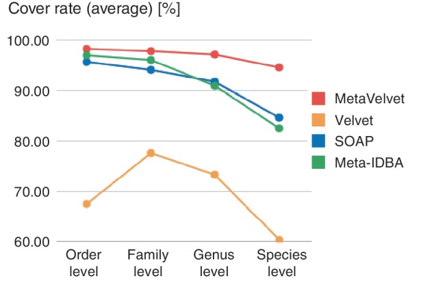
Cover rates for every taxonomic level are shown. The cover rate for each taxonomic level is the average of the cover rates for the 20 genomes in the taxonomic level.

Figure 8.

Detailed analysis of cover rates for 20 genomes in the genus level. Cover rates for each genome are listed in the order of species abundance.

Figure 8 shows the cover rates for 20 genomes with different abundances at the genus level. MetaVelvet achieved uniformly higher cover rates on all abundances. On the other hand, Velvet completely failed to reconstruct low-abundance species, and SOAPdenovo and Meta-IDBA showed low cover rates for certain species.

To verify that the MetaVelvet algorithm for identifying and separating the chimeric node actually works on a metagenome assembly, we concretely analyzed one of our experiments using the genus-level metagenomic dataset. On this dataset, MetaVelvet first detected nine peaks, that is, peaks 54, 41, 37, 21, 18, 16, 14, 12 and 6, in the node coverage distribution. Second, MetaVelvet identified 770 nodes as chimeric and separated them; 750 of those identified nodes were truly chimeric and the rest were incorrect. Two examples of chimeric nodes correctly identified by MetaVelvet are shown in Figure 9. The first example node was shared between the most dominant species of node coverage 54 and the third dominant species of node coverage 37. In contrast, an incorrect node misidentified by MetaVelvet is shown in the right example of Figure 9. This node was actually a repeat node. This misidentification of the chimeric node resulted from the statistical variance of k-mer frequencies that caused misassignment of peaks to the nodes. In conclusion, MetaVelvet produced longer N50 scores by successfully identifying and separating chimeric nodes.

Figure 9.

(A and B) Two examples of chimeric nodes correctly identified by MetaVelvet. (C) Example of a repeat node misidentified by MetaVelvet as chimeric.

The percentages of chimeric scaffolds of all assemblers were very small (at most 1.56%). MetaVelvet showed slightly higher chimera rates compared with SOAPdenovo and Meta-IDBA. These higher chimeric rates can be considered as a tradeoff against the longer scaffold sizes.

The longer N50 scores of the scaffolds particularly benefit the identification of protein-coding genes. Figure 10 clearly demonstrates this advantage: the number of predicted complete protein-coding genes from MetaVelvet scaffolds is significantly larger than any of the other assemblers at all taxonomic levels, where a complete protein-coding gene (complete ORF) denotes a gene (ORF) for which both of the 5′- and 3′-ends are included in a scaffold, and a partial genes (partial ORF) denotes a gene (ORF) whose 5′- and/or 3′-end is not included in a scaffold. In particular, the number of predicted genes from MetaVelvet scaffolds is more than twice that from Velvet scaffolds at the species level and is almost same as that from the separate assembly.

Figure 10.

The number of predicted complete protein-coding genes from scaffolds for each assembler.

In conclusion, the improvements gained by the MetaVelvet method strongly suggest that single-genome assemblers are not appropriate for metagenomic short read data. The MetaVelvet assembler can assemble metagenomic short read data with longer N50 sizes and can reconstruct scaffold sequences, even for low-abundance species.

Metagenomics analysis of human gut microbial data

To assess the assembly accuracy of the MetaVelvet assembler on real metagenomic datasets, we assembled three human gut microbial datasets, which were sequenced as a part of the MetaHIT project (3). Qin et al. (3) performed deep sequencing of fecal DNA samples obtained from 124 European adults. Assembly of the 124 human gut metagenomic datasets established a human gut microbial gene catalog. The work of Qin et al. (3) is an important milestone, which showed the potential effectiveness of metagenomic assembly of short reads. Here, human gut metagenomic datasets from three adults were selected (sample IDs are MH0006, MH0012 and MH0047) from the MetaHIT project and used to validate whether the MetaVelvet assembler could increase the number of protein-coding genes compared with a single-genome assembler, Velvet. Two datasets (MH0006 and MH0012) were the deepest and second-deepest datasets; the other dataset (MH0047) is one of the low-coverage datasets. The three metagenomic datasets were downloaded from the NCBI Sequence Read Archive (http://www.ncbi.nlm.nih.gov/sra; ERR011101–ERR011104 for the MH0006 dataset; ERR011117–ERR011123 for the MH0012 dataset; ERR011192–ERR011193 for the MH0047 dataset).

MetaVelvet was applied to the three datasets with a k-mer size set at 51. Figure 11 is the histogram of node coverages in the de Bruijn graph constructed from the MH0047 dataset, which clearly shows that multiple peaks were also observed in a real metagenomic dataset. Multiple peaks were observed in the MH0006 and MH0012 datasets (Supplementary Figures S1 and S2).

Figure 11.

Detection of multiple peaks on the node coverage histogram from the MH0047 human gut microbial dataset.

The assembly statistics of the three metagenomic datasets are summarized in Table 2. For comparison, Velvet was also applied to the three datasets with the k-mer size set at 51. MetaVelvet yielded significantly longer total scaffold lengths compared with Velvet. For the MH0006 dataset, MetaVelvet showed a 25% increase in total scaffold length, a 44% increase for MH0012 and a 51% increase for MH0047. From the scaffolds, the protein-coding genes were predicted using the MetaGene (23) software. 421 448 and 284 552 genes were predicted from MH0006 scaffolds assembled by MetaVelvet and Velvet, respectively, showing that MetaVelvet increased the number of predicted genes by 48.1%. Similarly, MetaVelvet increased the number of predicted genes by 106.5% for the MH0012 dataset and by 129.5% for the MH0047 dataset. More importantly, 90 617 and 84 811 complete genes were predicted from MH0006 scaffolds assembled by MetaVelvet and Velvet, respectively. This result showed that MetaVelvet increased the number of complete genes by 6.9% compared with a single-genome assembler Velvet. Similarly, MetaVelvet increased the number of complete genes by 10.1% for the MH0012 dataset and by 22.8% for the MH0047 dataset. These results evidently demonstrated that MetaVelvet substantially increased both the number of predicted genes and the number of complete genes.

Table 2.

Assembly and gene prediction statistics for human gut microbial metagenomic datasets

	MH0006		MH0012		MH0047
	MetaVelvet	Velvet	MetaVelvet	Velvet	MetaVelvet	Velvet
Scaffolds
Num. scaffolds	293 805	174 794	368 879	125 387	69 380	21 833
Total scaffold length (bp)	176534 240	141 464 165	239 717742	166 824 609	39 488 884	26 190 998
AUC of N-len(x)	1 740 532	764 099	5 049 858	1 897 179	280 526	181 960
AUCmin of N-len(x)	1 732 914	764 099	5 027 177	1 897 179	277 057	181 960
Protein-coding genes
Num. genes	421 448	284 552	531 824	257 502	92 411	40 267
Num. complete genes	90 617	84 811	129 670	117 792	18 032	14 680

AUC of N-len(x) denotes the area under the curve of the generalized score N-len(x), which is defined by Eq. (2), for 0 < x ≤ L. AUC_min of N-len(x) denotes the area under the curve of N-len(x) for 0 < x ≤ min{L, L′}.

To investigate how MetaVelvet yielded a larger number of genes, we analyzed the following generalized score of N50:

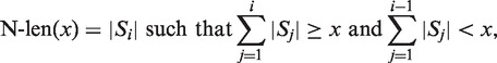(2)

where S₁, S₂, … , S_n denote the list of scaffolds in descending order of length as output by an assembler. Note that the N50 score (Eq. (1)) corresponds to the N-len(x) score for x = L/2, where L denotes the total scaffold length. When the total scaffold lengths of two assemblies are quite different in the human gut microbial datasets, the naive use of N50 score is inadequate, because even for the same lists of scaffolds in descending order, the longer L decreases the N50 score at L/2. This generalized score N-len(x) is more appropriate to compare scaffold integrity than the raw N50 score. Figure 12 shows the N-len(x) plot for the MH0012 scaffolds assembled by MetaVelvet and Velvet, showing that MetaVelvet greatly improved the scaffold integrity compared with Velvet. For example, when x = 1 000 000, the N-len(x) score of MetaVelvet was 345 388, while the N-len(x) of Velvet was 84 683. Further, we calculated the area under the curve (AUC) of N-len(x) for 0 < x ≤ L in units of 1 000 000 bp, that is, the cumulative sum of N-len(x) scores (0 < x ≤ L), where L denotes the total scaffold length. To eliminate the effect of L on calculating the AUC (that is, the longer L could likely increase the AUC), we also define the AUC_min of N-len(x) to be the AUC of N-len(x) for 0 < x ≤ min{L, L′}, where L is the total scaffold length of the one assembler and L′ is that of the other assembler. The AUC and AUC_min of N-len(x) of MetaVelvet were 5 049 858 and 5 027 177, respectively, for the MH0012 dataset, although the AUC and AUC_min of Velvet were both 1 897 179. These results imply that MetaVelvet achieved much longer scaffolds by factor of three compared with Velvet. Similarly, MetaVelvet showed greater scaffold integrity than Velvet for the MH0006 and MH0047 datasets (Supplementary Figures S3 and S4). This improvement in scaffold integrity represents the main reason why MetaVelvet yields a larger number of genes from metagenomic short read assemblies.

Figure 12.

N-len(x) plot of Eq. (2).

SUMMARY AND DISCUSSION

This study described an extension of the single-genome assembler Velvet to a metagenome assembler, MetaVelvet, and showed its effectiveness in several experiments using simulated datasets and human gut microbial sequence datasets. This work is the first step in the construction of a de novo metagenome assembler for the assembly of metagenomes from mixed ‘short’ sequence reads of multiple species.

Meta-IDBA (6) is a currently available and practically executable de novo metagenome assembler. From the results using the simulated datasets, it can be seen that MetaVelvet outperformed Meta-IDBA. In fact, the Meta-IDBA project (6) pointed out that one of their future works is to make use of uneven abundance ratios in metagenomic datasets. On the other hand, Meta-IDBA is designed to solve the metagenome assembly problem caused by polymorphisms in similar species in metagenomic environments. In this aspect, Meta-IDBA might be more useful for analyzing slight variants in the genomes of subspecies within a same species. Figure 13 shows the comparisons of the N50 scores of contigs between MetaVelvet assemblies and Meta-IDBA assemblies. Since Meta-IDBA does not have the scaffolding function, this result shows a fair comparison on assembly performances between both assemblers. Nevertheless, MetaVelvet achieved higher N50 scores than Meta-IDBA at the order, family and genus levels. On the other hand, Meta-IDBA produced higher N50 score for contigs at the species level, which confirms the specific feature of Meta-IDBA mentioned above.

Figure 13.

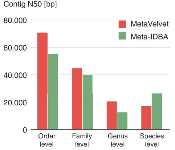
N50 scores for contigs generated by MetaVelvet and Meta-IDBA.

Although we have designed the primary procedure for MetaVelvet, a key issue is how to identify and deal with ambiguous nodes, termed chimeric nodes in this article, with multiple incoming and outgoing edges in the de Bruijn graph. Most nodes in the de Bruijn graph are unique nodes with only one incoming edge and one outgoing edge, and as such, are reliable for building contigs. The single-genome assemblers recognize the ambiguous nodes as repeat nodes, where a repeat node represents a sequence that occurs several times in the genome, which is correct in single-genome assembly. MetaVelvet explicitly identifies chimeric nodes as causing misassemblies that combine reads from distinct species to generate chimeric scaffolds. MetaVelvet then identifies and separates the chimeric node into two unique nodes using node coverage differences. The results showed that this simple strategy worked well for metagenome assembly. The results demonstrate that MetaVelvet is a potentially valuable tool that can be widely used in metagenomic analyses. In particular, a significant increase of the number of predicted complete protein-coding genes is valuable in the search for novel enzymes in metagenome research.

AVAILABILITY

The Supplementary Data are also available at: http://metavelvet.dna.bio.keio.ac.jp/supple.pdf.

SUPPLEMENTARY DATA

Supplementary Data are available at NAR Online: Supplementary Tables 1–4 and Supplementary Figures 1–4.

FUNDING

KAKENHI from the Ministry of Education, Culture, Sports, Science and Technology of Japan [Grant-in-Aid for Scientific Research on Innovative Areas No.221S0002]. A grant program for bioinformatics research and development of the Japan Science and Technology Agency (in part). Funding for open access charge: KAKENHI from the Ministry of Education, Culture, Sports, Science and Technology of Japan [Grant-in-Aid for Scientific Research on Innovative Areas No.221S0002].

Conflict of interest statement. None declared.

REFERENCES

- 1.Venter JC, Remington K, Heidelberg JF, Halpern AL, Rusch D, Eisen JA, Wu D, Paulsen I, Nelson KE, Nelson W, et al. Environmental genome shotgun sequencing of the Sargasso Sea. Science. 2004;304:66–74. doi: 10.1126/science.1093857. [DOI] [PubMed] [Google Scholar]
- 2.Kurokawa K, Itoh T, Kuwahara T, Oshima K, Toh H, Toyoda A, Takami H, Morita H, Sharma VK, Srivastava TP, et al. Comparative metagenomics revealed commonly enriched gene sets in human gut microbiomes. DNA Res. 2007;14:169–181. doi: 10.1093/dnares/dsm018. [DOI] [PMC free article] [PubMed] [Google Scholar]
- 3.Qin J, Li R, Raes J, Arumugam M, Burgdorf KS, Manichanh C, Nielsen T, Pons N, Levenez F, Yamada T, et al. A human gut microbial gene catalogue established by metagenomic sequencing. Nature. 2010;464:59–65. doi: 10.1038/nature08821. [DOI] [PMC free article] [PubMed] [Google Scholar]
- 4.Hiatt JB, Patwardhan RP, Turner EH, Lee C, and Shendure J. Parallel, tag-directed assembly of locally derived short sequence reads. Nat. Methods. 2010;7:119–122. doi: 10.1038/nmeth.1416. [DOI] [PMC free article] [PubMed] [Google Scholar]
- 5.Chen K, Pachter L. Bioinformatics for whole-genome shotgun sequencing of microbial communities. PLoS Comput. Biol. 2005;1:106–112. doi: 10.1371/journal.pcbi.0010024. [DOI] [PMC free article] [PubMed] [Google Scholar]
- 6.Peng Y, Leung HC, Yiu SM, Chin FY. Meta-IDBA: a de novo assembler for metagenomic data. Bioinformatics. 2011;27:i94–i101. doi: 10.1093/bioinformatics/btr216. [DOI] [PMC free article] [PubMed] [Google Scholar]
- 7.Laserson J, Jojic V, Koller D. Genovo: de novo assembly for metagenomes. J. Comput. Biol. 2011;18:429–443. doi: 10.1089/cmb.2010.0244. [DOI] [PubMed] [Google Scholar]
- 8.Charuvaka A, Rangwala H. Proceedings of Bioinformatics and Biomedicine (BIBM), 2010 IEEE International Conference. 2010. Evaluation of short read metagenomic assembly; pp. 171–178. [Google Scholar]
- 9.Ye Y, Tang H. An ORFome assembly approach to metagenomics sequences analysis. J. Bioinform. Comput. Biol. 2009;7:455–471. doi: 10.1142/s0219720009004151. [DOI] [PMC free article] [PubMed] [Google Scholar]
- 10.Saeed I, Halgamuge SK. The oligonucleotide frequency derived error gradient and its application to the binning of metagenome fragments. BMC Genomics. 2009;10(Suppl. 3):S10. doi: 10.1186/1471-2164-10-S3-S10. [DOI] [PMC free article] [PubMed] [Google Scholar]
- 11.Yang B, Peng Y, Leung HC, Yiu SM, Chen JC, Chin FY. Unsupervised binning of environmental genomic fragments based on an error robust selection of l-mers. BMC Bioinformatics. 2010;11(Suppl. 2):S5. doi: 10.1186/1471-2105-11-S2-S5. [DOI] [PMC free article] [PubMed] [Google Scholar]
- 12.Wu YW, Ye Y. A novel abundance-based algorithm for binning metagenomic sequences using l-tuples. J. Comput. Biol. 2011;18:523–534. doi: 10.1089/cmb.2010.0245. [DOI] [PMC free article] [PubMed] [Google Scholar]
- 13.Kunin V, Copeland A, Lapidus A, Mavromatis K, Hugenholtz P. A bioinformatician's guide to metagenomics. Microbiol. Mol. Biol. Rev. 2008;72:557–578. doi: 10.1128/MMBR.00009-08. [DOI] [PMC free article] [PubMed] [Google Scholar]
- 14.Nishito Y, Osana Y, Hachiya T, Popendorf K, Toyoda A, Fujiyama A, Itaya M, Sakakibara Y. Whole genome assembly of a natto production strain Bacillus subtilis natto from very short read data. BMC Genomics. 2010;11:243. doi: 10.1186/1471-2164-11-243. [DOI] [PMC free article] [PubMed] [Google Scholar]
- 15.Zerbino DR, Birney E. Velvet: algorithms for de novo short read assembly using de Bruijn graphs. Genome Res. 2008;18:821–829. doi: 10.1101/gr.074492.107. [DOI] [PMC free article] [PubMed] [Google Scholar]
- 16.Zerbino DR, McEwen GK, Margulies EH, Birney E. Pebble and rock band: heuristic resolution of repeats and scaffolding in the velvet short-read de novo assembler. PLoS One. 2009;4:e8407. doi: 10.1371/journal.pone.0008407. [DOI] [PMC free article] [PubMed] [Google Scholar]
- 17.Idury RM, Waterman MS. A new algorithm for DNA sequence assembly. J. Comput. Biol. 1995;2:291–306. doi: 10.1089/cmb.1995.2.291. [DOI] [PubMed] [Google Scholar]
- 18.Pevzner PA, Tang H, Waterman MS. An Eulerian path approach to DNA fragment assembly. Proc. Natl Acad. Sci. USA. 2001;98:9748–9753. doi: 10.1073/pnas.171285098. [DOI] [PMC free article] [PubMed] [Google Scholar]
- 19.Maccallum I, Przybylski D, Gnerre S, Burton J, Shlyakhter I, Gnirke A, Malek J, McKernan K, et al. ALLPATHS 2: small genomes assembled accurately and with high continuity from short paired reads. Genome Biol. 2009;10:R103. doi: 10.1186/gb-2009-10-10-r103. [DOI] [PMC free article] [PubMed] [Google Scholar]
- 20.Simpson JT, Wong K, Jackman SD, Schein JE, Jones SJ, Birol I. ABySS: a parallel assembler for short read sequence data. Genome Res. 2009;19:1117–1123. doi: 10.1101/gr.089532.108. [DOI] [PMC free article] [PubMed] [Google Scholar]
- 21.Lander ES, Waterman MS. Genomic mapping by fingerprinting random clones: a mathematical analysis. Genomics. 1988;2:231–239. doi: 10.1016/0888-7543(88)90007-9. [DOI] [PubMed] [Google Scholar]
- 22.Li R, Zhu H, Ruan J, Qian W, Fang X, Shi Z, Li Y, Li S, Shan G, Kristiansen K, et al. De novo assembly of human genomes with massively parallel short read sequencing. Genome Res. 2010;20:265–272. doi: 10.1101/gr.097261.109. [DOI] [PMC free article] [PubMed] [Google Scholar]
- 23.Noguchi H, Park J, Takagi T. MetaGene: prokaryotic gene finding from environmental genome shotgun sequences. Nucleic Acids Res. 2006;34:5623–5630. doi: 10.1093/nar/gkl723. [DOI] [PMC free article] [PubMed] [Google Scholar]
- 24.Unterseher M, Jumpponen A, Opik M, Tedersoo L, Moora M, Dormann CF, Schnittler M. Species abundance distributions and richness estimations in fungal metagenomics — lessons learned from community ecology. Mol. Ecol. 2011;20:275–285. doi: 10.1111/j.1365-294X.2010.04948.x. [DOI] [PubMed] [Google Scholar]
Associated Data
This section collects any data citations, data availability statements, or supplementary materials included in this article.