Network Rhythms Influence the Relationship between Spike-Triggered Local Field Potential and Functional Connectivity

Abstract

Characterizing the functional connectivity between neurons is key for understanding brain function. We recorded spikes and local field potentials (LFPs) from multielectrode arrays implanted in monkey visual cortex to test the hypotheses that spikes generated outward-traveling LFP waves and the strength of functional connectivity depended on stimulus contrast, as described recently. These hypotheses were proposed based on the observation that the latency of the peak negativity of the spike-triggered LFP average (STA) increased with distance between the spike and LFP electrodes, and the magnitude of the STA negativity and the distance over which it was observed decreased with increasing stimulus contrast. Detailed analysis of the shape of the STA, however, revealed contributions from two distinct sources—a transient negativity in the LFP locked to the spike (∼0 ms) that attenuated rapidly with distance, and a low-frequency rhythm with peak negativity ∼25 ms after the spike that attenuated slowly with distance. The overall negative peak of the LFP, which combined both these components, shifted from ∼0 to ∼25 ms going from electrodes near the spike to electrodes far from the spike, giving an impression of a traveling wave, although the shift was fully explained by changing contributions from the two fixed components. The low-frequency rhythm was attenuated during stimulus presentations, decreasing the overall magnitude of the STA. These results highlight the importance of accounting for the network activity while using STAs to determine functional connectivity.

Introduction

To understand how neural networks process information, it is crucial to characterize their connectivity pattern. The local field potential (LFP), as recorded with high-impedance (small contact size) microelectrodes, is thought to reflect synaptic activity in the vicinity of the microelectrode (Mitzdorf, 1985; Nunez and Srinivasan, 2006; Katzner et al., 2009; Khawaja et al., 2009) and could potentially provide a measure of the strength of connectivity between neurons. In particular, the spike-triggered average of the LFP (termed STA) is used to assess the strength of postsynaptic activity at one cortical site caused by spiking at another location (Jin et al., 2008; Nauhaus et al., 2009). Recently, Nauhaus et al. (2009) used an array of microelectrodes implanted in primary visual cortex (V1) of anesthetized monkeys and cats to explore functional connectivity. They fixed one electrode as the reference site for spiking and computed the STA for each microelectrode in the array. From the STA, they estimated the peak (negative) amplitude and the time at which the peak occurred relative to the generating spike (termed “time-to-peak” here). The time-to-peak increased with increasing distance between the reference (spike) and LFP electrodes, suggesting that the spikes were generating radial traveling waves in the LFP. Further, the STA amplitude was much larger during spontaneous activity than during strong visual stimulation, suggesting that the strength of functional connectivity depended on stimulus contrast.

At face value, these observations suggest that the STA might be a powerful tool for exploring functional connectivity and the interactions of local cortical circuit. However, while the traveling wave hypothesis explains why the time-to-peak increases with distance, it does not explain all the results. In particular, the LFP wave in the STA started ∼100 ms before the spike onset (i.e., the wave was noncausal), even in electrodes several millimeters away from the reference (spike) electrode. Because the LFP wave could be well approximated by one cycle of the alpha rhythm (∼8 Hz), which is prominent during spontaneous periods (Palva and Palva, 2007), we explored a solution based on ongoing oscillatory activity that could explain the shift in the peak of the LFP wave as well as its noncausal nature.

We found that spikes during the prestimulus period tended to occur ∼25 ms before the negative peak of an ongoing low-frequency (<10 Hz) rhythm, such that the STA showed two local negative peaks: one at 0 ms reflecting events associated with the spike, and a second at ∼25 ms reflecting the reliable timing of spikes relative to the low-frequency rhythm. The first peak was large for the reference electrode but decreased quickly with distance, while the second peak decreased much more slowly with distance. The overall peak therefore shifted from ∼0 to ∼25 ms with distance, giving an impression of a traveling wave. During strong visual stimulation, the low-frequency rhythm was greatly attenuated, reducing the STA amplitude and making it detectable over shorter distances. These observations call into question the suggestions that spikes generate traveling waves of LFP activity and the strength of functional connectivity changes with stimulus contrast.

Materials and Methods

Behavioral task and recording.

The animal protocols used in this study were approved by the Institutional Animal Care and Use Committee of Harvard Medical School. Recordings were made from two male rhesus monkeys (Macaca mulatta; 11 and 14 kg). Before training, a scleral search coil and a head post were implanted under general anesthesia. After monkeys learned the behavioral task (∼4 months), we implanted a 10 × 10 array of microelectrodes (96 active electrodes, Blackrock Microsystems) in V1 in the right cerebral hemisphere (∼15 mm from the occipital ridge and 15 mm lateral from the midline). The microelectrodes were 1 mm long and 400 μm apart, with impedance between 0.3 and 1 MΩ at 1 kHz. The receptive fields of the neurons recorded from the microelectrodes were in the lower left visual quadrant and centered between 3° and 5° eccentricity. Other findings based on data recorded from these arrays and animals have been reported previously (Ray and Maunsell, 2010, 2011).

The monkeys performed an orientation-change detection task (Task 1 in Ray and Maunsell, 2010). The monkey was required to hold its gaze within 1° of a small central dot (0.05–0.10° diameter) located at the center of a CRT video display (100 Hz refresh rate, 1280 × 768 pixels, gamma corrected), while two achromatic odd-symmetric Gabor stimuli were synchronously flashed for 400 ms with a mean interstimulus period of 600 ms. One stimulus was centered on the receptive field of one of the recorded sites (new location for each session); the second stimulus was located at an equal eccentricity on the opposite side of the fixation point. The Gabor stimuli were static with an SD of 0.5° and a spatial frequency of 4 cycles per degree at the preferred orientation of the selected recording site. The monkey was cued to attend to one stimulus location or the other in blocks of trials. The contrasts of the attended and unattended stimuli were equal on each presentation, and could take the following eight possible values: 0, 1.6, 3.1, 6.2, 12.5, 25, 50, and 100%, chosen pseudorandomly. At an unsignaled time drawn from an exponential distribution (Monkey 1: mean 2000 ms, range 1000–7000 ms; Monkey 2: mean 3000 ms, range 1000–7000 ms), the orientation of the stimulus at the cued location changed by 90°. The monkey was rewarded with a drop of juice for making a saccade to the location of the changed stimulus within 500 ms of the orientation change.

Monkeys 1 and 2 performed the task in 10 and 17 recording sessions. We analyzed only correct trials when the monkey was attending outside the receptive field. For each correct trial, only responses to stimuli after the first stimulus in the sequence and before the target were used for analysis, so that the stimulus conditions were identical for the entire dataset. On average, each stimulus was repeated 79 times (range 56–101 times) for Monkey 1 and 76 times (range 47–120 times) for Monkey 2.

Electrode selection.

Some electrodes in the array yielded weak and inconsistent responses and were excluded from analysis. For Monkey 1, one region of the array did not yield usable signals. The data reported here were obtained from 27 electrodes in Monkey 1 and 62 electrodes in Monkey 2. Each of these electrodes yielded reliable responses and stable estimates of the receptive field centers (SD <0.1° across days, mapped by flashing small Gabor stimuli on a rectangular grid that spanned the receptive fields of all the electrodes). Only electrodes with reliable estimates of the receptive field center were used so that we could limit the stimulus period analysis to sites within 0.2° of the stimulus center (see next paragraph). This analysis also provided an independent measure of the signal quality recorded from each electrode. In comparison, Nauhaus et al. (2009) used electrodes for which the time-to-peak versus distance plots were significant (p < 0.001), thereby removing all electrodes that failed to provide supporting evidence for traveling waves.

For the prestimulus STA, any electrode from which at least 25 spikes were obtained was used for analysis. For Monkey 1, this yielded 116 electrodes from 10 recording sessions (23 unique electrodes—many electrodes were recorded on multiple sessions; median spikes per electrode per session, 314; interquartile range, 111–778). For Monkey 2, this yielded 655 electrodes from 17 sessions (60 unique electrodes; median spikes, 236; interquartile range, 89–596 spikes). For stimulus STA, we used electrodes from which at least 25 spikes were obtained, and whose receptive fields were within 0.2° of the center of the stimulus. For Monkeys 1 and 2, this yielded 22 electrodes (12 unique; median spikes, 193; interquartile range, 75–335 spikes) and 46 electrodes (31 unique; median spikes, 98; interquartile range, 45–185 spikes). To account for the multiplicity of some electrodes, the STAs from the same electrode were averaged across sessions.

LFPs and multiunits were extracted using commercial hardware and software (Blackrock Microsystems). Raw data were filtered between 0.3 Hz (Butterworth filter, first-order, analog) and 500 Hz (Butterworth filter, fourth-order, digital) to extract the LFP, and digitized at 2 kHz (16 bit resolution). Multiunits were extracted by filtering the raw signal between 250 Hz (Butterworth filter, fourth-order, digital) and 7500 Hz (Butterworth filter, third-order, analog) followed by an amplitude threshold (set at ∼6.25 and ∼4.25 of the signal SD for the two monkeys). To improve the quality of the isolation, the multiunits were further sorted offline (Offline Sorter, Plexon Inc), although the results were similar when unsorted multiunits were used. LFP was used either raw (no additional filtering) or after filtering between 3 and 90 Hz or between 15 and 90 Hz (fourth-order high-pass and fifth-order low-pass Butterworth filters; filtered twice in original and time-reversed order to achieve zero phase distortion). The LFP from each electrode was independently z-scored. Because the spikes for STA computation were taken at a fixed time relative to stimulus onset, the stimulus-locked LFP signal (i.e., the evoked response) was subtracted from each LFP trace before the STA computation.

Space constant.

The amplitude of the STA (x) was related to the interelectrode distance (d) using the following equation:

where λ is termed “space constant” here. From x and d, the parameters M, λ, and B were fitted using least-squares minimization (see Figs. 2, 4). We also fitted M and λ after first fixing B to a prespecified value (following Nauhaus et al., 2009) (see Fig. 5).

Figure 2.

Population STA analysis during the prestimulus period. A, Average data of 23 reference sites in Monkey 1, as a function of distance between spike and LFP electrodes (indicated on the left), when raw LFP (filtered between 0.3 and 500 Hz) was used. The number of STAs averaged for each trace is shown on the right. B, The top plot shows the peak negative amplitude as a function of cortical distance between spike and LFP electrodes. The legend shows the space constant. The lower plot shows the time-to-peak negativity as a function of distance. The inverse of the slope (speed of propagation) and the significance of the regression fit are shown in the legend. C, D, Same as in A and B after first filtering the LFPs between 3 and 90 Hz. E–H, Same as in A–D for 60 reference electrodes in Monkey 2.

Figure 4.

No traveling waves in V1. A, B, Same as the plots shown in Figure 2, A and B, but for LFP filtered between 15 and 90 Hz. C, Top plot shows the time of the positive peak between 0 and 200 ms in the STA filtered between 3 and 90 Hz (as shown in Fig. 2C), as a function of cortical distance between spike and LFP electrodes. Lower plot shows the positive peak in the STA between −200 and 0 ms. D, Histogram of time-to-peak negativity values for all interelectrode distances up to 0.8 mm (left) or at 0.4 mm (right). The red lines show the best-fitting bimodal Gaussian distribution (see Results for details). For the right plot, the peak near 0 ms has a value of 0.16 (truncated at 0.1 to highlight the second peak). E–H, Same as in A–D for 60 electrodes in Monkey 2. For the histograms (H), the peaks of the Gaussians near time 0 had values of 0.25 and 0.43, which were truncated at 0.1 to highlight the second peak near ∼25 ms.

Figure 5.

Comparison of STAs during prestimulus versus stimulus-driven states. A, Average power spectra of LFP segments taken between 200 and 400 ms after stimulus onset (orange trace) and prestimulus periods (300–100 ms before stimulus onset; gray trace) for 12 electrodes in Monkey 1. Power is given in units of microvolt square per hertz [(μV)² Hz⁻¹]. B, Average STAs obtained from spikes recorded in the driven state for different interelectrode ranges (same format as in Fig. 2C). The gray trace shows the STA for the reference electrode (d = 0) using spikes recorded from the prestimulus condition. C, Amplitude versus distance (upper plot) for both the driven (orange circles; space constant shown in violet) and prestimulus conditions (gray; space constants shown in red and green; see text for details). The bottom row shows the time of the negative peak during the driven condition as a function of cortical distance from the spike electrode. The legend indicates the speed of propagation and the significance of the regression fit. D–F, Same as in A–C for 31 electrodes in Monkey 2.

Coherency analysis.

The coherency spectrum between two signals, x and y, is defined as

where S_xy(f) denotes the cross-spectrum, and S_xx(f) and S_yy(f) denote the auto-spectra of each signal. These were computed using the multitaper method (Thomson, 1982), implemented in Chronux 2.0 (Mitra and Bokil, 2008), an open-source data analysis toolbox available at http://chronux.org. Essentially, the multitaper method reduces the variance of spectral estimates by premultiplying the data with several orthogonal tapers known as Slepian functions. Details and properties of this method can be found elsewhere (Mitra and Pesaran, 1999; Jarvis and Mitra, 2001). We used a single taper to maximize the frequency resolution.

All circular statistics were performed using an open-source circular statistics toolbox CircStat2010 (Berens and Velasco, 2009).

Results

The results are organized as follows. First, we illustrate a mechanism that explains both the shift in the overall negative peak of the LFP with increasing electrode distance as well as the onset of the LFP wave before the spike itself (termed the “double-peak” hypothesis to distinguish it from the “traveling wave” hypothesis) (Fig. 1), and we show that this mechanism is difficult to visualize when the LFP is low-pass filtered. The STA analysis before stimulus onset is shown next (Figs. 2, 3) followed by tests to distinguish between the two hypotheses (Fig. 4). Finally, we describe the effect of visual stimulation on the STA (Fig. 5).

Figure 1.

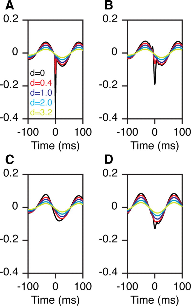
A mechanism that explains both the shift in the negative peak of the STA as well as its onset before time 0. A, The LFP has an ongoing oscillation at 8 Hz and spikes tend to occur 25 ms before its negative peak. The STA of the reference electrode (black trace) shows the contribution of the spike (sharp Gaussian with an SD of 2 ms centered at 0) and of the 8 Hz rhythm. The degree of phase locking determines the relative magnitudes of the two sources (arbitrarily chosen to be 0.4 and 0.08 for the spike transient and alpha rhythm). These two sources fall off at different rates with distance (d), depending on the degree of synchronization in the spikes and phase consistency of the alpha rhythm (space constants arbitrarily chosen to be 0.3 and 3 mm for the spike transient and alpha rhythm). B, Same data as in A, but filtered between 3 and 90 Hz, which decreases the spike transient but not the alpha rhythm. C, Same as in A, filtered between 3 and 20 Hz. D, STA (filtered between 3 and 90 Hz) for which spikes occur 10 ms before the negative peak of the rhythm. The spike transient (before filtering) and the rhythm both have a magnitude of 0.1.

Figure 3.

Coherence analysis during prestimulus period. A, Field–field coherence between LFPs recorded from the spike electrode and other electrodes, for different interelectrode distances, for 23 spike electrodes in Monkey 1 (same format as Fig. 2). The coherence of the reference electrode with itself (black trace) is not visible because it is unity at all frequencies. B, Spike-field coherence between the spikes recorded from the reference electrode and LFP recorded from other electrodes. C, Normalized histogram of the phase values at 5 Hz, obtained from the spike-field coherence analysis shown in B. The ticks on the left show the circular mean of the phase values for each interelectrode range. D–F, Same as in A–C for 60 reference electrodes in Monkey 2.

Double-peak hypothesis

The double-peak hypothesis is based on the following three assumptions: (1) there is an internal rhythm (such as an alpha rhythm) that is present across the entire network whose spatial coherence falls off with distance; (2) spikes are phase locked to this rhythm, appearing preferentially at a certain time before the trough of the rhythm; and (3) spike-related transients are present in the LFP and occur at almost zero delay with respect to the spike. These transients could be due to the synaptic events leading to the spike and the low-frequency component of the spike itself (i.e., spike bleed-through) (Ray et al., 2008; Ray and Maunsell, 2011).

To illustrate how different weighting of two waveforms with offset peaks can produce the appearance of a traveling wave, we simulated LFPs composed of two distinct components. During periods of spontaneous activity, the LFP is dominated by prominent low-frequency alpha rhythms, which we simulated by a sinusoid at 8 Hz in Figure 1A. Further, we assumed that spikes tended to occur 25 ms before the trough of the alpha rhythm. Each spike-related transient was simulated by a negative Gaussian with an SD of 2 ms. Note that the relative magnitudes of the alpha rhythm and sharp transient in the STA depend on the degree of phase locking, which could be arbitrary. For example, in our recordings the magnitude of the low-frequency rhythm in the STA was ∼10 μV, even though in the raw LFP it was hundreds of microvolts, suggesting that phase locking between the spike and the alpha rhythm was weak (Fig. 3). The STA from the reference electrode (the electrode used to establish spike triggering) showed prominent peaks at 0 and 25 ms for the spike transient and the alpha rhythm, respectively (Fig. 1A, black trace).

Both the spike transient and the alpha rhythm decreased in magnitude when the STA was computed from LFPs obtained from distant electrodes, but they decreased at different rates. For the alpha rhythm, the amplitude falloff depends on the phase consistency in these oscillations as a function of distance. If the oscillations are perfectly uniform and synchronized across cortex, the amplitude should not decrease with distance. However, in our data the phase consistency (measured using LFP–LFP coherence) decreased with increasing distance at all frequencies (Fig. 3). Consequently, the phases of the LFP segments that were averaged to get the STA were more random at larger interelectrode distances, leading to more reduction in the overall magnitude. On the other hand, the magnitude of the spike-related transient at other electrodes depends on the degree of synchronization between the spikes near that electrode and the spikes recorded from the reference electrode. We observed in our data that the magnitude fell off at a much faster rate than the alpha magnitude, which we illustrated in Figure 1A by using a space constant (λ in Eq. 1) that was 10 times smaller than the space constant of the alpha component. The magnitude of the spike transient also depends on the tuning preferences of the spike and LFP electrodes—if two electrodes have similar tuning, their activity will be more synchronized and the spike transient will have larger magnitude.

In Figure 1A, the overall peak of the STA is either at 0 ms (for electrodes near the reference) or 25 ms (for electrodes far away). If the STA estimates are noisy (as with physiological measurements), the measurements of the overall STA peak would be scattered around ∼0 and 25 ms, but would nonetheless remain bimodal. This bimodality is harder to observe when the LFP is low-pass filtered, which decreases, but does not eliminate, the spike transient. Figure 1B shows the same STAs filtered between 3 and 90 Hz. The two peaks are visible but less distinct. Figure 1C shows the same STAs filtered between 3 and 20 Hz. Now there appears to be a single peak moving progressively from 15 to 25 ms. The two peaks are also harder to visualize if spikes are locked closer to the trough of the alpha rhythm. For example, in Figure 1D, a spike transient that is comparable in magnitude to the alpha rhythm occurs 10 ms before its trough. The negative peak of the STA (filtered between 3 and 90 Hz) moves from 0 to 10 ms, although the two peaks are hard to distinguish. These simulations demonstrate that differential contributions from two components with peaks at different times can produce the illusion of a traveling wave where none exists.

Data analysis

We explored whether this effect occurs in neurophysiological signals by analyzing data recorded using electrode arrays implanted in monkey V1. STAs during prestimulus periods were computed using spikes that occurred 300–100 ms before stimulus onset. We selected one electrode as the reference site for spiking, and computed the STA of the LFP signals across all the electrodes in the array (27 and 62 electrodes for the two monkeys; see Materials and Methods for details). The LFP was used either raw (no additional filtering beyond the original filtering between 0.3–500 Hz) or filtered between 3 and 90 Hz, and was individually z-scored (Nauhaus et al., 2009). Similar results were obtained when the LFP was not z-scored.

Figure 2, A and E, show the population STAs of the raw LFP signal for five interelectrode ranges for the two monkeys. These plots include data from all days (23 and 60 reference electrodes from 10 and 17 recording sessions for the two monkeys; see Materials and Methods for details). The reference STA (black trace) showed a clear negative peak at 0 ms. The magnitude of this peak fell off quickly with increasing distance between spike and LFP electrodes. These plots also show a low-frequency component with a trough at ∼25 ms. The magnitude of this component fell off much more slowly with distance. Figure 2, B and F, show the amplitudes and time-to-peak as a function of distance for the entire dataset (points at each unique interelectrode distance were averaged for clarity). For the time-to-peak versus distance plot, both monkeys showed a significantly positive slope, with speeds (inverse slope) of 0.25 and 0.49 m/s. When the analysis was performed separately for each reference electrode, the median slope for Monkey 1 was 3.4 ± 0.9 s/m (SD was computed using bootstrapping), which was significantly greater than 0 (p = 0.01, sign rank test; N = 23). We averaged slopes instead of speeds because speed becomes infinite for a slope of 0. A slope of 3.4 corresponds to a speed of 0.30 m/s. For Monkey 2, the median slope was 2.15 ± 1.3 (p = 0.027, sign rank test; N = 60; speed, 0.47 m/s). For Monkey 2, the low-frequency rhythm was weak, so that for distances greater than ∼2 mm the peak negativity was difficult to estimate (Fig. 2F, bottom plot). The minimum value in such cases depends on the interval over which the minimum is computed, and on average equals the midpoint of the interval (0 ms in this case, because the interval was between −100 and 100 ms). We therefore also computed the slopes by taking the interelectrode distances only up to 2 mm. The median slope for the reduced dataset was 10.1 ± 1.8 s/m (p = 1.2 × 10⁻⁶, sign rank test; N = 60; speed, 0.1 m/s). These speeds are in the same range as reported in the earlier study (Nauhaus et al., 2009). We fitted an exponential to the amplitude versus distance plots (Eq. 1). The amplitude fell off with a median space constant (λ) of 0.32 ± 0.11 mm for Monkey 1 and 0.33 ± 0.05 for Monkey 2 when the asymptote (B) was used as a free parameter (i.e., not fixed to a prespecified value). These values are different from the values reported by Nauhaus et al. (2009), for reasons discussed later in the Results.

Because earlier findings were based on filtered LFP data (Nauhaus et al., 2009), we also examined the STA after first filtering the LFP between 3 and 90 Hz (Fig. 2C,D,G,H). The results were similar, although the filtering left the two peaks less distinct in the STA traces. Monkey 1 had a median slope of 2.5 ± 0.6 s/m (p = 4.9 × 10⁻⁴, sign rank test; N = 23; speed, 0.4 m/s). For Monkey 2, the median slope was 1.9 ± 0.9 s/m (p = 0.16, sign rank test; N = 60; speed, 0.53 m/s), which increased to 8.5 ± 1.8 (p = 4.2 × 10⁻⁵, sign rank test; N = 60; speed, 0.12 m/s) when only the electrodes within 2 mm of the reference electrode were used. The median space constants were 0.47 ± 0.31 and 0.32 ± 0.05 for the two monkeys.

We further tested the presence of a low-frequency rhythm and its phase locking with spikes using coherence analysis (Fig. 3). Figure 3, A and D, show the field–field coherence, which is a measure of the phase consistency between the LFPs measured from the reference electrode and other electrodes (measured using the multitaper method; see Eq. 2 for details), averaged over five interelectrode ranges (same format as in Fig. 2). The coherence values were high at low frequencies, with phase values close to 0 (i.e., the oscillations were synchronous at low frequencies) (data not shown). However, we did not observe a distinct peak. This could be due to the poor spectral resolution of the coherence measure (we used the LFP of 200 ms duration and therefore had a frequency resolution of 5 Hz) or could be due to arrhythmic behavior (i.e., a combination of wide-band slow fluctuations with high power). Similar results were obtained when we computed the spectral power (Fig. 5A,D, gray traces). The coherence values decreased with increasing interelectrode distance at all frequencies.

We next studied the degree of phase locking between spikes and LFP oscillations using the spike-field coherence (Fig. 3B,E). This measure showed a sharp peak at 5 Hz, suggesting that spikes were locked to a 5 Hz oscillation (at 5 Hz resolution). The normalized histograms of the phase values at this frequency are shown in Figure 3, C and F. For this plot, we first binned the phase values for each interelectrode range into 12 intervals (30° apart) and divided them by the maximum across the 12 values. The circular mean phases for Monkey 1 were 154, 155, 153, 146, and 144° for the five interelectrode ranges, and 147, 141, 139, 135, and 134° for Monkey 2 (Fig. 3C,F, ticks). The phases appeared to shift away from 180° (trough of the rhythm) with increasing interelectrode distance, especially for Monkey 2. This shows a serious problem with using coherence analysis without accounting for the sharp transient related to the spike. Based on this analysis, we could conclude that the trough of the low-frequency rhythm moved away relative to the spike (i.e., a traveling wave), or information could be coded relative to the position of the spike within the rhythmic cycle (phase coding). These conclusions are incorrect, because this apparent phase shift is due only to the presence of a sharp transient at 0, which can be decomposed as a series of sinusoids with a phase of 180° at all frequencies, and consequently moves the overall phase toward 180° (depending on its magnitude relative to the rhythm).

At large interelectrode distances, for which the spiking transient was negligible, the mean phases were 145 and 135° for the two monkeys, or a phase shift of 35 and 45° relative to the trough. For a 5 Hz sinusoid, this corresponds to a shift of 19 and 25 ms relative to the spike, very close to the values shown in Figure 2. Together, Figures 2 and 3 show that all the three assumptions for the double-peak hypothesis are met in these data.

The existence of two peaks that attenuate over different distances is consistent with the double-peak hypothesis, and raises the possibility that there is no traveling wave, only a gradual shift in dominance from one peak to the other. We performed three analyses that further suggest this is the case. First, we repeated the analysis described above after filtering the LFP between 15 and 90 Hz to eliminate the low-frequency peak (Fig. 4A,B,E,F). In this case, the slopes should be 0 with an offset at ∼0 ms, which was indeed the case. The median slopes were indistinguishable from 0: 2.8 ± 4.7 s/m (p = 0.68, sign rank test; N = 23) for Monkey 1 and 0.32 ± 1.7 s/m (p = 0.9, sign rank test; N = 60) for Monkey 2.

Second, we examined the positive peaks of the STA. For a traveling wave, there should be no activity before the spike onset, and the time of the positive peak after the spike should increase with distance in the same way as the negative peak. In contrast, a positive peak before the spike is consistent with the double-peak hypothesis, which further predicts that the time of the positive peaks should not change with distance (Fig. 1B). We found two positive peaks in the STA, which occurred at approximately ±100 ms (Fig. 2C,G). The top and bottom plots of Figure 4C show the time-to-peak of the two maxima in Figure 2C, computed between 0 and 200 ms and −200 and 0 ms, respectively. The slopes were not significantly different from 0. When computed separately for each reference electrode, the median slopes were 0.5 ± 1.0 s/m (p = 0.4, sign rank test; N = 23) and −0.46 ± 1.1 s/m (p = 1, sign rank test; N = 23). For Monkey 2 (Fig. 4G), the slopes were significantly negative for the pooled data. This is again due to the small magnitude of the positive peaks at large distances (Fig. 2G), so that the time-to-peak values shifted toward the midpoint of the analysis interval (100 and −100 ms for the top and bottom plots). When computed individually for each reference electrode, however, the median slopes for the two maxima were −1.8 ± 1.4 s/m (p = 0.052, sign rank test; N = 60) and −1.4 ± 2.6 s/m (p = 0.52, sign rank test; N = 60), with neither slope significantly different from 0. Visual inspection of Figure 2, C and G, confirmed that there was no obvious shift in the latencies of the maxima. The same trends are visible in the STAs shown by Nauhaus et al. (2009; their Fig. 2). A waveform with positive peaks that are fixed in time and bracket a negative peak that shifts in time is consistent with the double-peak hypothesis, and is difficult to reconcile with a traveling wave.

Third, the distribution of time-to-peak values at a fixed electrode distance should be unimodal if they arise from a traveling wave, but may appear bimodal if they arise from differing combinations of two component peaks at ∼0 and ∼25 ms. Figure 4, D and H (left panels), show normalized histograms of the time-to-peak values for all electrodes within 0.8 mm of the reference electrode. Two peaks are visible at ∼0 and ∼25 ms. These distributions were fitted with either a unimodal or a bimodal Gaussian distribution (using the GM distribution function in Matlab) and the Akaike information criterion (AIC) was used as a measure of the goodness of fit. For both monkeys, using two Gaussians yielded a lower AIC value than a single Gaussian, suggesting that the bimodal fit was better than the unimodal. For the bimodal distribution, the means of two Gaussians were at 5 and 22 ms for Monkey 1, and at 4 and 31 ms for Monkey 2. The results were similar when only the smallest interelectrode distance was used (d = 0.4 mm) (Fig. 4D,H, right panels), although they were harder to see because of low sample size. For this reduced dataset also, a bimodal Gaussian distribution provided a better fit than a unimodal, with the peaks of the Gaussians at 5 and 24 ms for Monkey 1, and at 4 and 29 ms for Monkey 2. In comparison, the peaks of Gaussians fitted on time-to-peak values obtained from electrodes ≥2 mm away from the reference electrode were 26 and 28 ms for the two monkeys. Thus, even at the smallest nonzero interelectrode distance, the second peak in the histogram was very close to the peak obtained at large interelectrode distances.

Collectively, these results show that there are two peaks in the STA at ∼0 and ∼25 ms, and that with increasing electrode distance there is only a shift in the dominance from the first peak to the second, rather than a progression of intermediate peak times that would be associated with a traveling wave.

Effect of visual stimulation on STA magnitude

The preceding analyses were based on neuronal activity recorded when no stimulus was presented. Next, we tested the claim that traveling waves were smaller and more spatially restricted during visual stimulation, which was interpreted as a signature of a decreased strength of functional connectivity. We analyzed the STA when spikes were taken 200–400 ms after the onset of a full-contrast stimulus (this time range was chosen to avoid the transient activity after stimulus onset). Figure 5, A and D, show the average power spectra of the LFP between 200 and 400 ms after stimulus onset (orange traces) and 300–100 ms before stimulus onset (gray traces), recorded from 12 and 31 electrodes for the two monkeys (see Materials and Methods for details). After stimulus onset, LFP power decreased at lower frequencies and increased at higher frequencies. In particular, we observed a salient gamma rhythm at ∼50 Hz during the stimulus period.

The STA magnitude during the stimulus period critically depended on the magnitude of the gamma rhythm, which was much weaker for Monkey 1 compared with Monkey 2. Figure 5B shows the STAs computed during the stimulus period as a function of interelectrode distance (same format as Fig. 2C; note the difference in scale on the time axis) for Monkey 1, together with the STA during prestimulus activity for the reference electrode (gray trace). Because the low-frequency rhythm was attenuated after stimulus onset, amplitude of the STA decreased (Fig. 5B, gray vs black traces). The space constant for the amplitude versus distance plot for the stimulus period (Fig. 5C, upper plot, orange circles) was 0.74 mm for the entire dataset from this animal. When computed for each reference electrode separately, the median space constant was 0.60 ± 3.4 mm. For the prestimulus condition (gray circles), the median space constant was 0.34 ± 0.40 mm when the asymptote was a free parameter (red trace). However, if the space constant was determined after fixing the asymptote to the value obtained from the stimulus condition (Nauhaus et al., 2009, green trace), a much larger value was obtained (median, 4.3 ± 1.2 mm).

For Monkey 2, the gamma rhythm was strong, so the STA amplitude was larger during the stimulus period than the prestimulus period (Fig. 5E, gray vs black traces). The median space constant was 0.89 ± 0.22 mm for the stimulus period and 0.34 ± 0.10 mm during the prestimulus period when the asymptote was a free parameter. When fixed to the asymptote obtained during stimulus condition (which was typically larger than the prestimulus period), the space constants were infinite. This shows the serious problem that arises when the asymptotes are fixed for two different conditions. This issue is considered further in the Discussion.

For the stimulus condition, slopes of the time-to-peak versus distance plots (Fig. 5C,F, bottom plots) were not significantly different from 0 for either monkey (Monkey 1: median, 4.3 ± 2.9 s/m; p = 0.39, sign rank test; N = 12; Monkey 2: median, −0.84 ± 2.2 s/m; p = 1, sign rank test; N = 31), with a y-axis intercept near 0 ms.

Discussion

Different components in the STA

The spike-triggered LFP average, by definition, shows all activity that is locked to spikes. This includes signals arising from synaptic activity associated with the spike (e.g., presynaptic and postsynaptic currents in the spiking neuron and current produced by the spike), but also includes any activity that biases the timing of the spikes, such as the different network rhythms associated with various behavioral and stimulus conditions.

The feedforward synaptic input to V1 neurons due to spiking activity in the thalamus, which has been characterized by simultaneously recording from both areas, reveals a sharp transient signal of a few milliseconds duration (Jin et al., 2008). However, because we recorded both spikes and LFP from V1, our STAs show both the synaptic input as well as the low-frequency component of the action potential waveform. It is not possible to dissociate between these two sources in the extracellular signal. We call this the “spike transient” because both these events are immediately associated with the recorded spike, regardless of the network state, and are characterized by a sharp depolarization near time 0. The sharp negativity can be well represented by a Gaussian with a small sigma (resembling a delta function) (Ray et al., 2008). Note that the spike component has more power at lower frequencies than higher frequencies (Fourier transform of a Gaussian with a small sigma is a Gaussian with large sigma), but its power at lower frequencies is masked out by the much larger “1/f” noise in the LFP, so that its contribution is visible only above ∼50 Hz in the raw LFP (Ray and Maunsell, 2011). This signal has power in a broad frequency range and therefore cannot be extracted by traditional filtering mechanisms. STAs from other electrodes show part of this component due to common input and correlated firing (i.e., synaptic inputs and spikes that are synchronized with the spike recorded from the reference electrode). However, the magnitude of this component decreases and there could also be a broadening of the Gaussian as the degree of synchronization falls with distance.

In addition to these events associated with the spike, there are network oscillations that potentially arise from a different subpopulation of neurons. For example, the gamma rhythm is thought to be generated by a network of inhibitory interneurons (Bartos et al., 2007; Cardin et al., 2009; Sohal et al., 2009), which provide a rhythmic barrage of IPSPs and can modulate the time at which a pyramidal neuron could fire within the gamma cycle (Hasenstaub et al., 2005). Similarly, low-frequency alpha rhythms (8–12 Hz) are thought to be generated by layer-specific pyramidal neurons acting as local pacemakers (Bollimunta et al., 2008). If spikes occur preferentially at a certain phase of these rhythms, the rhythm will be captured in the STA, and its magnitude will depend on the strength of phase locking.

Both the spike component and the network rhythms depend on many factors. An increase in the degree of synchronization may increase the magnitude of the spike component, such as for electrodes with same orientation preference. The low-frequency alpha component is severely attenuated by visual stimulation (Palva and Palva, 2007). Both the magnitude and center frequency of the gamma rhythm depend critically on stimulus properties, such as contrast (Henrie and Shapley, 2005; Ray and Maunsell, 2010), orientation (Frien et al., 2000; Berens et al., 2008; Lima et al., 2010), size (Gieselmann and Thiele, 2008), speed (Gray and Viana Di Prisco, 1997; Friedman-Hill et al., 2000), direction (Liu and Newsome, 2006), and cross-orientation suppression (Lima et al., 2010). All these factors could influence the magnitude and time-to-peak of the STA.

The double-peak hypothesis

An earlier report suggested that spikes generate traveling waves in the LFP and that changes in the magnitude of these waves reflected changes in functional connectivity (Nauhaus et al., 2009). A prominent difference between the current data and the previous report is that the space constants during spontaneous periods differ greatly. Because stimuli were presented rapidly in our protocol, STAs computed during the prestimulus condition may not be equivalent to the STAs computed during prolonged spontaneous periods. However, as described above, the discrepancy in the space constants likely arises because the asymptotes for spontaneous periods were fixed to the asymptotes for the stimulus period in their analysis. Our space constants were similar to their values when we also fixed the asymptotes (for Monkey 1). Note that the expected value for the STA amplitude is 0 at large interelectrode distances. Measured values, however, can depend on the number of spikes used to compute the STA—fewer spikes may result in a noisy STA whose global minima may not be small. Thus, even in the absence of any rhythmic network activity, the asymptotes for spontaneous and driven states could differ due to differences in the number of spikes used for STA computation. As described in the Results, when rhythmic activity is present in the network, the amplitude falloff could depend on the phase consistency in these oscillations as a function of distance. Other differences that could affect the space constants are the type of stimulus (full field vs small stimuli) and the short duration of our prestimulus and stimulus periods, which could lead to stimulus-locked effects related to attention or expectancy.

Another major difference between the studies is that our monkeys were awake and performing an attention task, while their monkeys were anesthetized. Anesthesia can have a pronounced effect on brain activity (Rojas et al., 2006; Potez and Larkum, 2008). During anesthesia, the network could be in a more synchronized state, and the spikes could represent the activity of local pacemakers generating a low-frequency rhythm (which could partially explain the traveling wave they observed). However, the un-normalized magnitudes of the STAs were similar for the two studies (∼15 and ∼8 μV for Monkeys 1 and 2 in our data, compared with ∼12 μV in their data), and other results (speeds, space constants, and the degree of noncausality of the STAs) were comparable when the data were analyzed using similar methods.

The noncausality of the STA is a major concern for the traveling wave hypothesis. Nauhaus et al. (2009) attributed this to correlation in space (i.e., common input) (Lampl et al., 1999) and time (i.e., spike autocorrelations), and to the band-limited nature of the LFP signal. We observed the same noncausality when the LFP was not filtered beyond the real-time, causal filtering between 0.3 and 500 Hz by the data collection device, which rules out the second possibility. The first possibility—spatial and temporal events correlated with the spike—is very similar to the idea we propose (in our case, these spatially and temporally correlated events constitute the alpha/gamma rhythms). However, the STA is large even before time 0, suggesting that the contribution from these spatially/temporally correlated events is larger than the contribution made by the synaptic events leading to the spike (which could be a marker of the functional connectivity). Moreover, with visual stimulation the reduction of these correlated events (alpha rhythms) decreases the magnitude of the STA, not the size of the synaptic event associated with the spike. Thus, whether or not spikes potentially generate an event that travels with distance, the decrease in the magnitude of the STA during visual stimulation cannot be attributed to a change in functional connectivity.

Other observations

As described in the Results, traveling waves during prestimulus activity and the decrease in STA magnitude during visual stimulation can be explained by the presence of network oscillations during prestimulus and stimulus-driven states. Further, because spikes provide information about the phase of the ongoing oscillatory activity, they can be used to predict the LFP (Nauhaus et al., 2009, their Fig. 3; note that the prediction decreases with increasing frequency, as shown in their Fig. 3c). This is consistent with other studies where the phase of the ongoing oscillations <10 Hz was found to be a significant predictor of the multiunit firing (Belitski et al., 2008, 2010; Montemurro et al., 2008; Rasch et al., 2008; Whittingstall and Logothetis, 2009). Finally, sites with similar orientation preferences have higher correlation in spikes due to more common input (Kohn and Smith, 2005; Smith and Kohn, 2008). This would increase the magnitude of the spike transient of the sites that have the same orientation preference as the reference electrode [Nauhaus et al. (2004), their Fig. 4].

In summary, our results show that it is inappropriate to simply use the magnitude of the STA as a measure of synaptic strength. The STA captures many features of the network, which must be separated before conclusions can be drawn. Separating out the spiking or synaptic events from ongoing rhythmic activity remains a major technical challenge in the field, which must be addressed before conclusions can be drawn from the analysis of local fields in the brain.

References

- Bartos M, Vida I, Jonas P. Synaptic mechanisms of synchronized gamma oscillations in inhibitory interneuron networks. Nat Rev Neurosci. 2007;8:45–56. doi: 10.1038/nrn2044. [DOI] [PubMed] [Google Scholar]
- Belitski A, Gretton A, Magri C, Murayama Y, Montemurro MA, Logothetis NK, Panzeri S. Low-frequency local field potentials and spikes in primary visual cortex convey independent visual information. J Neurosci. 2008;28:5696–5709. doi: 10.1523/JNEUROSCI.0009-08.2008. [DOI] [PMC free article] [PubMed] [Google Scholar]
- Belitski A, Panzeri S, Magri C, Logothetis NK, Kayser C. Sensory information in local field potentials and spikes from visual and auditory cortices: time scales and frequency bands. J Comput Neurosci. 2010;29:533–545. doi: 10.1007/s10827-010-0230-y. [DOI] [PMC free article] [PubMed] [Google Scholar]
- Berens P, Velasco MJ. Tübingen, Germany: Max Planck Institute for Biological Cybernetics; 2009. The circular statistics toolbox for Matlab. Technical report no. 184. [Google Scholar]
- Berens P, Keliris GA, Ecker AS, Logothetis NK, Tolias AS. Comparing the feature selectivity of the gamma-band of the local field potential and the underlying spiking activity in primate visual cortex. Front Syst Neurosci. 2008;2:2. doi: 10.3389/neuro.06.002.2008. [DOI] [PMC free article] [PubMed] [Google Scholar]
- Bollimunta A, Chen Y, Schroeder CE, Ding M. Neuronal mechanisms of cortical alpha oscillations in awake-behaving macaques. J Neurosci. 2008;28:9976–9988. doi: 10.1523/JNEUROSCI.2699-08.2008. [DOI] [PMC free article] [PubMed] [Google Scholar]
- Cardin JA, Carlén M, Meletis K, Knoblich U, Zhang F, Deisseroth K, Tsai LH, Moore CI. Driving fast-spiking cells induces gamma rhythm and controls sensory responses. Nature. 2009;459:663–667. doi: 10.1038/nature08002. [DOI] [PMC free article] [PubMed] [Google Scholar]
- Friedman-Hill S, Maldonado PE, Gray CM. Dynamics of striate cortical activity in the alert macaque: I. Incidence and stimulus-dependence of gamma-band neuronal oscillations. Cereb Cortex. 2000;10:1105–1116. doi: 10.1093/cercor/10.11.1105. [DOI] [PubMed] [Google Scholar]
- Frien A, Eckhorn R, Bauer R, Woelbern T, Gabriel A. Fast oscillations display sharper orientation tuning than slower components of the same recordings in striate cortex of the awake monkey. Eur J Neurosci. 2000;12:1453–1465. doi: 10.1046/j.1460-9568.2000.00025.x. [DOI] [PubMed] [Google Scholar]
- Gieselmann MA, Thiele A. Comparison of spatial integration and surround suppression characteristics in spiking activity and the local field potential in macaque V1. Eur J Neurosci. 2008;28:447–459. doi: 10.1111/j.1460-9568.2008.06358.x. [DOI] [PubMed] [Google Scholar]
- Gray CM, Viana Di Prisco G. Stimulus-dependent neuronal oscillations and local synchronization in striate cortex of the alert cat. J Neurosci. 1997;17:3239–3253. doi: 10.1523/JNEUROSCI.17-09-03239.1997. [DOI] [PMC free article] [PubMed] [Google Scholar]
- Hasenstaub A, Shu Y, Haider B, Kraushaar U, Duque A, McCormick DA. Inhibitory postsynaptic potentials carry synchronized frequency information in active cortical networks. Neuron. 2005;47:423–435. doi: 10.1016/j.neuron.2005.06.016. [DOI] [PubMed] [Google Scholar]
- Henrie JA, Shapley R. LFP power spectra in V1 cortex: the graded effect of stimulus contrast. J Neurophysiol. 2005;94:479–490. doi: 10.1152/jn.00919.2004. [DOI] [PubMed] [Google Scholar]
- Jarvis MR, Mitra PP. Sampling properties of the spectrum and coherency of sequences of action potentials. Neural Comput. 2001;13:717–749. doi: 10.1162/089976601300014312. [DOI] [PubMed] [Google Scholar]
- Jin JZ, Weng C, Yeh CI, Gordon JA, Ruthazer ES, Stryker MP, Swadlow HA, Alonso JM. On and off domains of geniculate afferents in cat primary visual cortex. Nat Neurosci. 2008;11:88–94. doi: 10.1038/nn2029. [DOI] [PMC free article] [PubMed] [Google Scholar]
- Katzner S, Nauhaus I, Benucci A, Bonin V, Ringach DL, Carandini M. Local origin of field potentials in visual cortex. Neuron. 2009;61:35–41. doi: 10.1016/j.neuron.2008.11.016. [DOI] [PMC free article] [PubMed] [Google Scholar]
- Khawaja FA, Tsui JM, Pack CC. Pattern motion selectivity of spiking outputs and local field potentials in macaque visual cortex. J Neurosci. 2009;29:13702–13709. doi: 10.1523/JNEUROSCI.2844-09.2009. [DOI] [PMC free article] [PubMed] [Google Scholar]
- Kohn A, Smith MA. Stimulus dependence of neuronal correlation in primary visual cortex of the macaque. J Neurosci. 2005;25:3661–3673. doi: 10.1523/JNEUROSCI.5106-04.2005. [DOI] [PMC free article] [PubMed] [Google Scholar]
- Lampl I, Reichova I, Ferster D. Synchronous membrane potential fluctuations in neurons of the cat visual cortex. Neuron. 1999;22:361–374. doi: 10.1016/s0896-6273(00)81096-x. [DOI] [PubMed] [Google Scholar]
- Lima B, Singer W, Chen NH, Neuenschwander S. Synchronization dynamics in response to plaid stimuli in monkey V1. Cereb Cortex. 2010;20:1556–1573. doi: 10.1093/cercor/bhp218. [DOI] [PMC free article] [PubMed] [Google Scholar]
- Liu J, Newsome WT. Local field potential in cortical area MT: stimulus tuning and behavioral correlations. J Neurosci. 2006;26:7779–7790. doi: 10.1523/JNEUROSCI.5052-05.2006. [DOI] [PMC free article] [PubMed] [Google Scholar]
- Mitra PP, Pesaran B. Analysis of dynamic brain imaging data. Biophys J. 1999;76:691–708. doi: 10.1016/S0006-3495(99)77236-X. [DOI] [PMC free article] [PubMed] [Google Scholar]
- Mitra P, Bokil H. New York: Oxford UP; 2008. Observed brain dynamics. [Google Scholar]
- Mitzdorf U. Current source-density method and application in cat cerebral cortex: investigation of evoked potentials and EEG phenomena. Physiol Rev. 1985;65:37–100. doi: 10.1152/physrev.1985.65.1.37. [DOI] [PubMed] [Google Scholar]
- Montemurro MA, Rasch MJ, Murayama Y, Logothetis NK, Panzeri S. Phase-of-firing coding of natural visual stimuli in primary visual cortex. Curr Biol. 2008;18:375–380. doi: 10.1016/j.cub.2008.02.023. [DOI] [PubMed] [Google Scholar]
- Nauhaus I, Busse L, Carandini M, Ringach DL. Stimulus contrast modulates functional connectivity in visual cortex. Nat Neurosci. 2009;12:70–76. doi: 10.1038/nn.2232. [DOI] [PMC free article] [PubMed] [Google Scholar]
- Nunez PL, Srinivasan R. 2nd Ed. New York: Oxford UP; 2006. Electric fields of the brain. [Google Scholar]
- Palva S, Palva JM. New vistas for [alpha]-frequency band oscillations. Trends Neurosci. 2007;30:150–158. doi: 10.1016/j.tins.2007.02.001. [DOI] [PubMed] [Google Scholar]
- Potez S, Larkum ME. Effect of common anesthetics on dendritic properties in layer 5 neocortical pyramidal neurons. J Neurophysiol. 2008;99:1394–1407. doi: 10.1152/jn.01126.2007. [DOI] [PubMed] [Google Scholar]
- Rasch MJ, Gretton A, Murayama Y, Maass W, Logothetis NK. Inferring spike trains from local field potentials. J Neurophysiol. 2008;99:1461–1476. doi: 10.1152/jn.00919.2007. [DOI] [PubMed] [Google Scholar]
- Ray S, Maunsell JH. Differences in gamma frequencies across visual cortex restrict their possible use in computation. Neuron. 2010;67:885–896. doi: 10.1016/j.neuron.2010.08.004. [DOI] [PMC free article] [PubMed] [Google Scholar]
- Ray S, Maunsell JH. Different origins of gamma rhythm and high-gamma activity in macaque visual cortex. PLoS Biol. 2011;9:e1000610. doi: 10.1371/journal.pbio.1000610. [DOI] [PMC free article] [PubMed] [Google Scholar]
- Ray S, Hsiao SS, Crone NE, Franaszczuk PJ, Niebur E. Effect of stimulus intensity on the spike-local field potential relationship in the secondary somatosensory cortex. J Neurosci. 2008;28:7334–7343. doi: 10.1523/JNEUROSCI.1588-08.2008. [DOI] [PMC free article] [PubMed] [Google Scholar]
- Rojas MJ, Navas JA, Rector DM. Evoked response potential markers for anesthetic and behavioral states. Am J Physiol Regul Integr Comp Physiol. 2006;291:R189–R196. doi: 10.1152/ajpregu.00409.2005. [DOI] [PubMed] [Google Scholar]
- Smith MA, Kohn A. Spatial and temporal scales of neuronal correlation in primary visual cortex. J Neurosci. 2008;28:12591–12603. doi: 10.1523/JNEUROSCI.2929-08.2008. [DOI] [PMC free article] [PubMed] [Google Scholar]
- Sohal VS, Zhang F, Yizhar O, Deisseroth K. Parvalbumin neurons and gamma rhythms enhance cortical circuit performance. Nature. 2009;459:698–702. doi: 10.1038/nature07991. [DOI] [PMC free article] [PubMed] [Google Scholar]
- Thomson DJ. Spectrum estimation and harmonic analysis. Proc IEEE. 1982;70:1055–1096. [Google Scholar]
- Whittingstall K, Logothetis NK. Frequency-band coupling in surface EEG reflects spiking activity in monkey visual cortex. Neuron. 2009;64:281–289. doi: 10.1016/j.neuron.2009.08.016. [DOI] [PubMed] [Google Scholar]